%matplotlib inline
from d2l import torch as d2l
from torch import nn
import torch
import torchvision
import os20.2 Fine-Tuning
In earlier chapters, we discussed how to train models on the Fashion-MNIST training dataset with only 60000 images. We also described ImageNet, the most widely used large-scale image dataset in academia, which has more than 10 million images and 1000 objects. However, the size of the dataset that we usually encounter is between those of the two datasets.
Suppose that we want to recognize different types of chairs from images, and then recommend purchase links to users. One possible method is to first identify 100 common chairs, take 1000 images of different angles for each chair, and then train a classification model on the collected image dataset. Although this chair dataset may be larger than the Fashion-MNIST dataset, the number of examples is still less than one-tenth of that in ImageNet. This may lead to overfitting of complicated models that are suitable for ImageNet on this chair dataset. Besides, due to the limited amount of training examples, the accuracy of the trained model may not meet practical requirements.
In order to address the above problems, an obvious solution is to collect more data. However, collecting and labeling data can take a lot of time and money. For example, in order to collect the ImageNet dataset, researchers have spent millions of dollars from research funding. Although the current data collection cost has been significantly reduced, this cost still cannot be ignored.
Another solution is to apply transfer learning to transfer the knowledge learned from the source dataset to the target dataset. For example, although most of the images in the ImageNet dataset have nothing to do with chairs, the model trained on this dataset may extract more general image features, which can help identify edges, textures, shapes, and object composition. These similar features may also be effective for recognizing chairs.
20.2.1 Steps
In this section, we will introduce a common technique in transfer learning: fine-tuning. As shown in Figure 20.2.1, fine-tuning consists of the following four steps:
- Pretrain a neural network model, i.e., the source model, on a source dataset (e.g., the ImageNet dataset).
- Create a new neural network model, i.e., the target model. This copies all model designs and their parameters on the source model except the output layer. We assume that these model parameters contain the knowledge learned from the source dataset and this knowledge will also be applicable to the target dataset. We also assume that the output layer of the source model is closely related to the labels of the source dataset; thus it is not used in the target model.
- Add an output layer to the target model, whose number of outputs is the number of categories in the target dataset. Then randomly initialize the model parameters of this layer.
- Train the target model on the target dataset, such as a chair dataset. The output layer will be trained from scratch, while the parameters of all the other layers are fine-tuned based on the parameters of the source model.
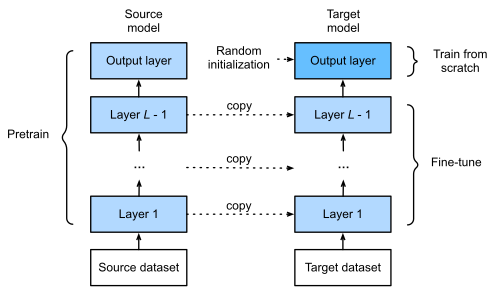
When target datasets are much smaller than source datasets, fine-tuning helps to improve models’ generalization ability.
20.2.2 Hot Dog Recognition
Let’s demonstrate fine-tuning via a concrete case: hot dog recognition. We will fine-tune a ResNet model on a small dataset, which was pretrained on the ImageNet dataset. This small dataset consists of thousands of images with and without hot dogs. We will use the fine-tuned model to recognize hot dogs from images.
%matplotlib inline
import os
from d2l import tensorflow as d2l
import tensorflow as tf
import keras%matplotlib inline
import os
from d2l import jax as d2l
from d2l.nnx_resnet import ResNet50, Bottleneck
from flax import nnx
import jax
from jax import numpy as jnp
import optax
import numpy as np
import tensorflow as tf # only used for tf.data input pipeline
# Activation (gradient) checkpointing. Fine-tuning ResNet-50 at batch size 128
# would otherwise hold the whole forward graph's activations live for the
# backward pass (~23 GB). Wrapping each residual block (`Bottleneck`) in
# `nnx.remat` recomputes that block's activations during backprop instead of
# storing them, cutting the peak to ~6 GB. `nnx.remat` propagates state
# correctly, so gradients and batch-norm running statistics are identical to
# the un-checkpointed model.
if not getattr(Bottleneck, '_d2l_remat', False):
Bottleneck.__call__ = nnx.remat(Bottleneck.__call__)
Bottleneck._d2l_remat = True%matplotlib inline
from d2l import mxnet as d2l
from mxnet import gluon, init, np, npx
from mxnet.gluon import nn
import os
npx.set_np()20.2.2.1 Reading the Dataset
The hot dog dataset we use was taken from online images. This dataset consists of 1400 positive-class images containing hot dogs, and as many negative-class images containing other foods. 1000 images of both classes are used for training and the rest are for testing.
After unzipping the downloaded dataset, we obtain two folders hotdog/train and hotdog/test. Both folders have hotdog and not-hotdog subfolders, either of which contains images of the corresponding class.
d2l.DATA_HUB['hotdog'] = (d2l.DATA_URL + 'hotdog.zip',
                         'fba480ffa8aa7e0febbb511d181409f899b9baa5')

data_dir = d2l.download_extract('hotdog')
We create two instances to read all the image files in the training and testing datasets, respectively.
train_imgs = torchvision.datasets.ImageFolder(os.path.join(data_dir, 'train'))
test_imgs = torchvision.datasets.ImageFolder(os.path.join(data_dir, 'test'))
from PIL import Image as _PILImage
import pathlib
def _load_image_folder(path):
"""Load images from a directory with class subfolders, returning
a list of (PIL.Image, class_index) tuples."""
path = pathlib.Path(path)
class_names = sorted([p.name for p in path.iterdir() if p.is_dir()])
class_to_idx = {c: i for i, c in enumerate(class_names)}
items = []
for cls in class_names:
for img_path in sorted((path / cls).iterdir()):
try:
img = _PILImage.open(str(img_path)).convert('RGB')
items.append((img, class_to_idx[cls]))
except Exception:
continue
return items
train_imgs = _load_image_folder(os.path.join(data_dir, 'train'))
test_imgs = _load_image_folder(os.path.join(data_dir, 'test'))# Load images as (PIL.Image, label) lists for compatibility with show_images
from PIL import Image as _PILImage
import pathlib

def _load_image_folder(path):
    """Load images from a directory with class subfolders, returning
    a list of (PIL.Image, class_index) tuples."""
    path = pathlib.Path(path)
    class_names = sorted([p.name for p in path.iterdir() if p.is_dir()])
    class_to_idx = {c: i for i, c in enumerate(class_names)}
    items = []
    for cls in class_names:
        for img_path in sorted((path / cls).iterdir()):
            try:
                img = _PILImage.open(str(img_path)).convert('RGB')
                items.append((img, class_to_idx[cls]))
            except Exception:
                continue
    return items

train_imgs = _load_image_folder(os.path.join(data_dir, 'train'))
test_imgs = _load_image_folder(os.path.join(data_dir, 'test'))train_imgs = gluon.data.vision.ImageFolderDataset(
os.path.join(data_dir, 'train'))
test_imgs = gluon.data.vision.ImageFolderDataset(
os.path.join(data_dir, 'test'))The first 8 positive examples and the last 8 negative images are shown below. As you can see, the images vary in size and aspect ratio.
hotdogs = [train_imgs[i][0] for i in range(8)]
not_hotdogs = [train_imgs[-i - 1][0] for i in range(8)]
d2l.show_images(hotdogs + not_hotdogs, 2, 8, scale=1.4);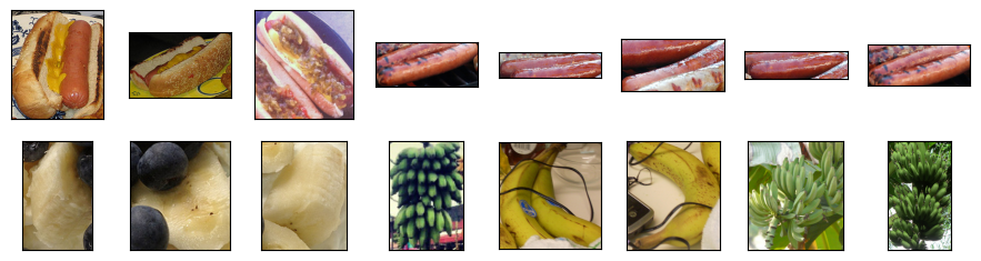
During training, we first crop a random area of random size and random aspect ratio from the image, and then scale this area to a \(224 \times 224\) input image. During testing, we scale both the height and width of an image to 256 pixels, and then crop a central \(224 \times 224\) area as input. In addition, for the three RGB (red, green, and blue) color channels we standardize their values channel by channel. Concretely, the mean value of a channel is subtracted from each value of that channel and then the result is divided by the standard deviation of that channel.
# Specify the means and standard deviations of the three RGB channels to
# standardize each channel
normalize = torchvision.transforms.Normalize(
    [0.485, 0.456, 0.406], [0.229, 0.224, 0.225])

train_augs = torchvision.transforms.Compose([
    torchvision.transforms.RandomResizedCrop(224),
    torchvision.transforms.RandomHorizontalFlip(),
    torchvision.transforms.ToTensor(),
    normalize])

test_augs = torchvision.transforms.Compose([
    torchvision.transforms.Resize([256, 256]),
    torchvision.transforms.CenterCrop(224),
    torchvision.transforms.ToTensor(),
    normalize])
# Plain tf.image / tf.data preprocessing for Keras ResNet50 (NHWC). Keras
# ResNet50 expects its own `preprocess_input` convention, not PyTorch-style
# RGB mean/std normalization.
IMG_SIZE = 224
def _normalize(x):
return tf.keras.applications.resnet50.preprocess_input(
tf.cast(x, tf.float32))
def train_augs(x, training=False):
# Input is (256, 256, 3) — already resized by image_dataset_from_directory.
x = tf.image.random_crop(x, (IMG_SIZE, IMG_SIZE, 3))
x = tf.image.random_flip_left_right(x)
return _normalize(x)
def test_augs(x, training=False):
# Input is (256, 256, 3) — already resized by image_dataset_from_directory.
# Center crop to IMG_SIZE x IMG_SIZE.
off = (256 - IMG_SIZE) // 2
x = x[off:off + IMG_SIZE, off:off + IMG_SIZE, :]
return _normalize(x)# Image preprocessing. We use `tf.image` ops so the pipeline can run
# inside `tf.data.Dataset.map`. The ImageNet RGB mean/std normalization
# matches the preprocessing expected by the pretrained ImageNet ResNet
# weights (and the PyTorch/MXNet tabs).
IMG_SIZE = 224
_IMAGENET_MEAN = tf.constant([0.485, 0.456, 0.406], dtype=tf.float32)
_IMAGENET_STD = tf.constant([0.229, 0.224, 0.225], dtype=tf.float32)
def _normalize(x):
return (tf.cast(x, tf.float32) / 255.0 - _IMAGENET_MEAN) / _IMAGENET_STD
def train_preprocess(x):
# `x` is a (256, 256, 3) float32 RGB image with values in [0, 255].
x = tf.image.random_crop(x, size=(IMG_SIZE, IMG_SIZE, 3))
x = tf.image.random_flip_left_right(x)
return _normalize(x)
def test_preprocess(x):
x = tf.image.resize_with_crop_or_pad(x, IMG_SIZE, IMG_SIZE)
return _normalize(x)# Specify the means and standard deviations of the three RGB channels to
# standardize each channel
normalize = gluon.data.vision.transforms.Normalize(
[0.485, 0.456, 0.406], [0.229, 0.224, 0.225])
train_augs = gluon.data.vision.transforms.Compose([
gluon.data.vision.transforms.RandomResizedCrop(224),
gluon.data.vision.transforms.RandomFlipLeftRight(),
gluon.data.vision.transforms.ToTensor(),
normalize])
test_augs = gluon.data.vision.transforms.Compose([
gluon.data.vision.transforms.Resize(256),
gluon.data.vision.transforms.CenterCrop(224),
gluon.data.vision.transforms.ToTensor(),
normalize])20.2.2.2 Defining and Initializing the Model
We use ResNet-18, which was pretrained on the ImageNet dataset, as the source model. Here, we specify pretrained=True to automatically download the pretrained model parameters. If this model is used for the first time, Internet connection is required for download.
We use ResNet-50, which was pretrained on the ImageNet dataset, as the source model. (Keras 3’s keras.applications does not ship a pretrained ResNet-18, so we use ResNet-50 here even though the PyTorch and MXNet tabs use ResNet-18.) Here, we specify weights='imagenet' to automatically download the pretrained model parameters. If this model is used for the first time, Internet connection is required for download.
We use an NNX ResNet-50 pretrained on ImageNet as the source model. Its official Microsoft safetensors are downloaded from Hugging Face and mapped directly into the stateful NNX model. If this model is used for the first time, Internet connection is required for download.
We use ResNet-18, which was pretrained on the ImageNet dataset, as the source model. Here, we specify pretrained=True to automatically download the pretrained model parameters. If this model is used for the first time, Internet connection is required for download.
pretrained_net = torchvision.models.resnet18(
    weights=torchvision.models.ResNet18_Weights.DEFAULT)
# Load pretrained ResNet50 (full model with top) to inspect the output layer
pretrained_net = keras.applications.ResNet50(weights='imagenet')_dummy = jnp.zeros((1, IMG_SIZE, IMG_SIZE, 3), dtype=jnp.float32)
pretrained_net = ResNet50.from_pretrained()pretrained_net = gluon.model_zoo.vision.resnet18_v2(pretrained=True)The pretrained source model instance contains a number of feature layers and an output layer fc. The main purpose of this division is to facilitate the fine-tuning of model parameters of all layers but the output layer. The member variable fc of source model is given below.
The pretrained ResNet50 from keras.applications contains a number of feature layers and an output layer. We will reuse the pretrained weights for transfer learning. The final layer of the source model is shown below.
The pretrained source model contains a convolutional backbone and a final fc layer (the 1000-way ImageNet classifier). The main purpose of this division is to facilitate the fine-tuning of model parameters of all layers but the output layer. The shape of the source model’s classifier weight is shown below.
The pretrained source model instance contains two member variables: features and output. The former contains all layers of the model except the output layer, and the latter is the output layer of the model. The main purpose of this division is to facilitate the fine-tuning of model parameters of all layers but the output layer. The member variable output of source model is shown below.
pretrained_net.fcLinear(in_features=512, out_features=1000, bias=True)pretrained_net.layers[-1]<Dense name=predictions, built=True>pretrained_net.fc.kernel.shape(2048, 1000)pretrained_net.outputDense(512 -> 1000, linear)As a fully connected layer, it transforms ResNet’s final global average pooling outputs into 1000 class outputs of the ImageNet dataset. We then construct a new neural network as the target model. It is defined in the same way as the pretrained source model except that its number of outputs in the final layer is set to the number of classes in the target dataset (rather than 1000).
In the code below, the model parameters before the output layer of the target model instance finetune_net are initialized to model parameters of the corresponding layers from the source model. Since these model parameters were obtained via pretraining on ImageNet, they are effective. Therefore, we can only use a small learning rate to fine-tune such pretrained parameters. In contrast, model parameters in the output layer are randomly initialized and generally require a larger learning rate to be learned from scratch. Letting the base learning rate be \(\eta\), a learning rate of \(10\eta\) will be used to iterate the model parameters in the output layer.
finetune_net = torchvision.models.resnet18(
    weights=torchvision.models.ResNet18_Weights.DEFAULT)
finetune_net.fc = nn.Linear(finetune_net.fc.in_features, 2)
nn.init.xavier_uniform_(finetune_net.fc.weight);
# Pretrained ResNet50 base (no top) + global average pool + fresh 2-class head
finetune_net = keras.Sequential([
keras.applications.ResNet50(weights='imagenet', include_top=False,
pooling='avg',
input_shape=(IMG_SIZE, IMG_SIZE, 3)),
keras.layers.Dense(2, kernel_initializer='glorot_uniform',
name='classifier'),
])finetune_net = ResNet50.from_pretrained()
finetune_net.fc = nnx.Linear(2048, 2, rngs=nnx.Rngs(1))finetune_net = gluon.model_zoo.vision.resnet18_v2(classes=2)
finetune_net.features = pretrained_net.features
finetune_net.output.initialize(init.Xavier())
# The model parameters in the output layer will be iterated using a learning
# rate ten times greater
for p in finetune_net.output.collect_params().values():
p.lr_mult = 1020.2.2.3 Fine-Tuning the Model
First, we define a training function train_fine_tuning that uses fine-tuning so it can be called multiple times.
# If `param_group=True`, the model parameters in the output layer will be
# updated using a learning rate ten times greater
def train_fine_tuning(net, learning_rate, batch_size=128, num_epochs=5,
                      param_group=True):
    train_iter = torch.utils.data.DataLoader(torchvision.datasets.ImageFolder(
        os.path.join(data_dir, 'train'), transform=train_augs),
        batch_size=batch_size, shuffle=True)
    test_iter = torch.utils.data.DataLoader(torchvision.datasets.ImageFolder(
        os.path.join(data_dir, 'test'), transform=test_augs),
        batch_size=batch_size)
    devices = d2l.try_all_gpus()
    loss = nn.CrossEntropyLoss(reduction="none")
    if param_group:
        params_1x = [param for name, param in net.named_parameters()
             if name not in ["fc.weight", "fc.bias"]]
        trainer = torch.optim.SGD([{'params': params_1x},
                                   {'params': net.fc.parameters(),
                                    'lr': learning_rate * 10}],
                                lr=learning_rate, weight_decay=0.001)
    else:
        trainer = torch.optim.SGD(net.parameters(), lr=learning_rate,
                                  weight_decay=0.001)
    d2l.train_ch13(net, train_iter, test_iter, loss, trainer, num_epochs,
                   devices)
def _make_tf_dataset(img_dir, augs, batch_size, shuffle=False):
"""Create a tf.data.Dataset from an image folder using Keras pipelines."""
ds = keras.utils.image_dataset_from_directory(
img_dir, label_mode='int', image_size=(256, 256),
batch_size=None, shuffle=shuffle)
ds = ds.map(lambda x, y: (augs(x, training=True), y),
num_parallel_calls=tf.data.AUTOTUNE)
ds = ds.batch(batch_size, drop_remainder=True).prefetch(tf.data.AUTOTUNE)
return ds
def _checkpointed_backbone(base):
"""Run the ResNet50 convolutional backbone with per-residual-block
activation checkpointing. A plain `tf.GradientTape` over ResNet-50 at batch
size 128 keeps every layer's activations live for the backward pass (~22 GB
of GPU memory). Splitting the backbone into its 16 residual blocks and
wrapping each in `tf.recompute_grad` recomputes a block's activations during
backprop instead of storing them, dropping the peak to a few GB. The
gradients are unchanged -- activations are simply traded for a little extra
compute. Returns a callable `fn(x, training) -> 2048-d pooled features`."""
boundaries = ['pool1_pool'] + [l.name for l in base.layers
if l.name.endswith('_out')]
segments = [keras.Model(base.input, base.get_layer(boundaries[0]).output)]
for a, b in zip(boundaries[:-1], boundaries[1:]):
segments.append(keras.Model(base.get_layer(a).output,
base.get_layer(b).output))
pool = keras.layers.GlobalAveragePooling2D()
def forward(x, training=False):
h = x
for seg in segments:
h = tf.recompute_grad(
lambda t, seg=seg: seg(t, training=training))(h)
return pool(h)
return forward
# If `param_group=True`, the head (classifier Dense) is updated with a
# learning rate ten times larger than the backbone, mirroring the PyTorch
# fine-tuning recipe. `momentum` is forwarded to both SGD optimizers; the
# from-scratch baseline uses momentum=0.9 because plain SGD cannot train a
# randomly-initialised ResNet-50 on 2 000 images in five epochs.
def train_fine_tuning(net, learning_rate, batch_size=128, num_epochs=5,
param_group=True, momentum=0.0):
train_ds = _make_tf_dataset(os.path.join(data_dir, 'train'),
train_augs, batch_size, shuffle=True)
test_ds = _make_tf_dataset(os.path.join(data_dir, 'test'),
test_augs, batch_size, shuffle=False)
# Backbone always trainable; discriminative LR (head at 10x) applied
# by routing gradients to two separate optimizers below.
net.layers[0].trainable = True
head_layer = net.layers[-1]
head_vars = head_layer.trainable_variables
head_var_ids = {id(v) for v in head_vars}
# Activation-checkpointed backbone (see `_checkpointed_backbone`); the
# classifier head is applied to its pooled features. Training still runs
# over `net.trainable_variables`, so the discriminative-LR split is intact.
backbone = _checkpointed_backbone(net.layers[0])
opt_head = keras.optimizers.SGD(
learning_rate=learning_rate * (10 if param_group else 1),
momentum=momentum, weight_decay=0.001)
opt_base = keras.optimizers.SGD(
learning_rate=learning_rate,
momentum=momentum, weight_decay=0.001)
loss_fn = keras.losses.SparseCategoricalCrossentropy(from_logits=True)
acc_metric = keras.metrics.SparseCategoricalAccuracy()
val_acc_metric = keras.metrics.SparseCategoricalAccuracy()
@tf.function
def train_step(x, y):
with tf.GradientTape() as tape:
logits = head_layer(backbone(x, training=True))
loss = loss_fn(y, logits)
grads = tape.gradient(loss, net.trainable_variables)
head_pairs, base_pairs = [], []
for g, v in zip(grads, net.trainable_variables):
if g is None:
continue
(head_pairs if id(v) in head_var_ids
else base_pairs).append((g, v))
if head_pairs:
opt_head.apply_gradients(head_pairs)
if base_pairs:
opt_base.apply_gradients(base_pairs)
acc_metric.update_state(y, logits)
return loss
@tf.function
def test_step(x, y):
logits = net(x, training=False)
val_acc_metric.update_state(y, logits)
for epoch in range(num_epochs):
acc_metric.reset_state()
val_acc_metric.reset_state()
total_loss, n_batches = 0.0, 0
for x, y in train_ds:
total_loss += float(train_step(x, y)); n_batches += 1
for x, y in test_ds:
test_step(x, y)
print(f'epoch {epoch + 1}, loss {total_loss / max(n_batches, 1):.3f}, '
f'train acc {float(acc_metric.result()):.3f}, '
f'test acc {float(val_acc_metric.result()):.3f}')def _make_tf_dataset(img_dir, preprocess, batch_size, shuffle=False):
"""Create a tf.data.Dataset from an image folder directory."""
ds = tf.keras.utils.image_dataset_from_directory(
img_dir, label_mode='int', image_size=(256, 256),
batch_size=None, shuffle=shuffle)
ds = ds.map(lambda x, y: (preprocess(x), y),
num_parallel_calls=tf.data.AUTOTUNE)
# Keep fixed shapes for training, but evaluate every test example.
ds = ds.batch(batch_size, drop_remainder=shuffle).prefetch(tf.data.AUTOTUNE)
return ds
# If `param_group=True`, the head is updated with a learning rate ten times
# larger than the pretrained backbone (mirroring the PyTorch tab); otherwise
# all parameters are trained at the same rate (used for `scratch_net`).
def train_fine_tuning(net, learning_rate, batch_size=128, num_epochs=5,
param_group=True, update_batch_stats=False,
momentum=0.0):
train_ds = _make_tf_dataset(os.path.join(data_dir, 'train'),
train_preprocess, batch_size, shuffle=True)
test_ds = _make_tf_dataset(os.path.join(data_dir, 'test'),
test_preprocess, batch_size, shuffle=False)
# Per-parameter learning rate: 10x for the new classifier, 1x for the
# pretrained backbone. Use a label tree to drive optax.multi_transform.
# Weight decay and optional momentum follow the comparison recipes below.
if param_group:
def labels(params):
return jax.tree_util.tree_map_with_path(
lambda path, _: ('head' if any(
(getattr(p, 'key', None) == 'fc' or
getattr(p, 'name', None) == 'fc') for p in path)
else 'base'), params)
tx = optax.multi_transform(
{'head': optax.chain(
optax.add_decayed_weights(0.001),
optax.sgd(learning_rate * 10, momentum=momentum)),
'base': optax.chain(
optax.add_decayed_weights(0.001),
optax.sgd(learning_rate, momentum=momentum))},
labels)
else:
tx = optax.chain(
optax.add_decayed_weights(0.001),
optax.sgd(learning_rate, momentum=momentum))
optimizer = nnx.Optimizer(net, tx, wrt=nnx.Param)
train_net = nnx.view(net, use_running_average=not update_batch_stats,
raise_if_not_found=False)
eval_net = nnx.view(net, use_running_average=True,
raise_if_not_found=False)
@nnx.jit
def train_step(model, optimizer, x, y):
def loss_fn(model):
logits = model(x)
loss = optax.softmax_cross_entropy_with_integer_labels(
logits, y).mean()
return loss, logits
(loss, logits), grads = nnx.value_and_grad(
loss_fn, has_aux=True)(model)
optimizer.update(model, grads)
acc = (jnp.argmax(logits, axis=-1) == y).mean()
return loss, acc
@nnx.jit
def eval_step(model, x, y):
logits = model(x)
return (jnp.argmax(logits, axis=-1) == y).sum()
for epoch in range(num_epochs):
total_loss, total_acc, n_batches = (jnp.array(0.0),
jnp.array(0.0), 0)
for x, y in train_ds:
x = jnp.asarray(x.numpy()); y = jnp.asarray(y.numpy())
loss, acc = train_step(train_net, optimizer, x, y)
total_loss += loss
total_acc += acc
n_batches += 1
test_correct, test_examples = jnp.array(0), 0
for x, y in test_ds:
x = jnp.asarray(x.numpy()); y = jnp.asarray(y.numpy())
test_correct += eval_step(eval_net, x, y)
test_examples += len(y)
total_loss, total_acc, test_correct = jax.device_get(
(total_loss, total_acc, test_correct))
print(f'epoch {epoch + 1}, loss {float(total_loss) / n_batches:.3f}, '
f'train acc {float(total_acc) / n_batches:.3f}, '
f'test acc {float(test_correct) / max(test_examples, 1):.3f}')
return netdef train_fine_tuning(net, learning_rate, batch_size=128, num_epochs=5):
train_iter = gluon.data.DataLoader(
train_imgs.transform_first(train_augs), batch_size, shuffle=True)
test_iter = gluon.data.DataLoader(
test_imgs.transform_first(test_augs), batch_size)
devices = d2l.try_all_gpus()
net.reset_ctx(devices)
net.hybridize()
loss = gluon.loss.SoftmaxCrossEntropyLoss()
trainer = gluon.Trainer(net.collect_params(), 'sgd', {
'learning_rate': learning_rate, 'wd': 0.001})
d2l.train_ch13(net, train_iter, test_iter, loss, trainer, num_epochs,
devices)We set the base learning rate to a small value in order to fine-tune the model parameters obtained via pretraining. Based on the previous settings, we will train the output layer parameters of the target model from scratch using a learning rate ten times greater.
train_fine_tuning(finetune_net, 5e-5)loss 0.163, train acc 0.940, test acc 0.943
1730.9 examples/sec on [device(type='cuda', index=0)]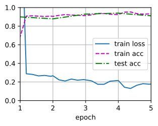
train_fine_tuning(finetune_net, 5e-5, momentum=0.9)Found 2000 files belonging to 2 classes.
Found 800 files belonging to 2 classes.
epoch 1, loss 0.820, train acc 0.517, test acc 0.751
epoch 2, loss 0.425, train acc 0.796, test acc 0.901
epoch 3, loss 0.279, train acc 0.895, test acc 0.915
epoch 4, loss 0.228, train acc 0.918, test acc 0.934
epoch 5, loss 0.212, train acc 0.923, test acc 0.941print('fine-tuned model')
finetune_net = train_fine_tuning(finetune_net, 1e-4, momentum=0.9)fine-tuned model
Found 2000 files belonging to 2 classes.
Found 800 files belonging to 2 classes.
epoch 1, loss 0.638, train acc 0.773, test acc 0.877
epoch 2, loss 0.524, train acc 0.918, test acc 0.911
epoch 3, loss 0.419, train acc 0.931, test acc 0.917
epoch 4, loss 0.342, train acc 0.942, test acc 0.921
epoch 5, loss 0.286, train acc 0.947, test acc 0.927# lr divided by batch_size: gluon Trainer no longer rescales (issue 7 fix in d2l.train_batch_ch13)
train_fine_tuning(finetune_net, 7.8125e-5)loss 0.279, train acc 0.915, test acc 0.921
282.7 examples/sec on [gpu(0)]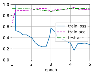
For comparison, we define an identical model, but initialize all of its model parameters to random values. Since the entire model needs to be trained from scratch, we can use a larger learning rate.
scratch_net = torchvision.models.resnet18()
scratch_net.fc = nn.Linear(scratch_net.fc.in_features, 2)
train_fine_tuning(scratch_net, 5e-4, param_group=False)
loss 0.379, train acc 0.837, test acc 0.836
1521.4 examples/sec on [device(type='cuda', index=0)]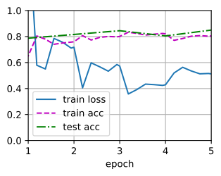
# Train from scratch: same architecture but with random (no-pretrain) weights.
scratch_base = keras.applications.ResNet50(
    weights=None, include_top=False, pooling='avg',
    input_shape=(IMG_SIZE, IMG_SIZE, 3))
# Keras' default BatchNormalization momentum (0.99) means the moving
# mean/variance never catch up to the actual activation statistics within
# five epochs of ~15 batches each, so the from-scratch model would look
# like random noise at evaluation time (train acc rises, test acc stays
# ~0.5). Lowering momentum to 0.5 lets the running stats track the small
# dataset; the pretrained fine-tuning path keeps the default because its
# moving stats are already calibrated on ImageNet.
for layer in scratch_base.layers:
    if isinstance(layer, keras.layers.BatchNormalization):
        layer.momentum = 0.5
scratch_net = keras.Sequential([
    scratch_base,
    keras.layers.Dense(2, kernel_initializer='glorot_uniform',
                       name='classifier'),
])
# Plain SGD (momentum=0) cannot train a randomly-initialised ResNet-50 on
# 2 000 images in five epochs, so we use SGD with momentum=0.9 and a single
# uniform learning rate (no head/backbone split) for the from-scratch run.
train_fine_tuning(scratch_net, 1e-3, param_group=False, momentum=0.9)
Found 2000 files belonging to 2 classes.
Found 800 files belonging to 2 classes.
epoch 1, loss 0.748, train acc 0.531, test acc 0.505
epoch 2, loss 0.754, train acc 0.573, test acc 0.562
epoch 3, loss 0.555, train acc 0.705, test acc 0.822
epoch 4, loss 0.410, train acc 0.815, test acc 0.833
epoch 5, loss 0.428, train acc 0.822, test acc 0.733print('scratch baseline')
scratch_net = ResNet50(num_classes=2, rngs=nnx.Rngs(2))
# On this tiny dataset the running statistics must adapt much faster than the
# ImageNet default.
scratch_net = nnx.view(scratch_net, momentum=0.5, raise_if_not_found=False)
scratch_net = train_fine_tuning(
scratch_net, 1e-3, num_epochs=6, param_group=False,
update_batch_stats=True, momentum=0.9)scratch baseline
Found 2000 files belonging to 2 classes.
Found 800 files belonging to 2 classes.
epoch 1, loss 0.709, train acc 0.530, test acc 0.504
epoch 2, loss 0.725, train acc 0.539, test acc 0.506
epoch 3, loss 0.588, train acc 0.682, test acc 0.522
epoch 4, loss 0.447, train acc 0.798, test acc 0.499
epoch 5, loss 0.406, train acc 0.810, test acc 0.500
epoch 6, loss 0.359, train acc 0.830, test acc 0.502scratch_net = gluon.model_zoo.vision.resnet18_v2(classes=2)
scratch_net.initialize(init=init.Xavier())
# lr divided by batch_size: gluon Trainer no longer rescales (issue 7 fix in d2l.train_batch_ch13)
train_fine_tuning(scratch_net, 7.8125e-4)loss 0.348, train acc 0.862, test acc 0.828
513.3 examples/sec on [gpu(0)]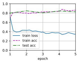
As we can see, the fine-tuned model reaches high accuracy in fewer epochs because its initial parameter values already encode useful visual features.
20.2.3 Summary
- Transfer learning transfers knowledge learned from the source dataset to the target dataset. Fine-tuning is a common technique for transfer learning.
- The target model copies all model designs with their parameters from the source model except the output layer, and fine-tunes these parameters based on the target dataset. In contrast, the output layer of the target model needs to be trained from scratch.
- Generally, fine-tuning parameters uses a smaller learning rate, while training the output layer from scratch can use a larger learning rate.
20.2.4 Exercises
- Keep increasing the learning rate of
finetune_net. How does the accuracy of the model change? - Further adjust hyperparameters of
finetune_netandscratch_netin the comparative experiment. Do they still differ in accuracy? - Set the parameters before the output layer of
finetune_netto those of the source model and do not update them during training. How does the accuracy of the model change? You can use the following code.
for param in finetune_net.parameters():
    param.requires_grad = False
# Freeze the ResNet50 backbone (layer 0 of the Sequential); only head trains.
finetune_net.layers[0].trainable = False# Freeze the pretrained ResNet-50 backbone; only the new `fc` head
# is updated by setting the optimizer learning rate of every other parameter
# to zero. For example, modify `train_fine_tuning` to use:
# optax.multi_transform(
# {'head': optax.sgd(lr * 10, momentum=0.9),
# 'base': optax.set_to_zero()},
# labels)for p in finetune_net.features.collect_params().values():
p.grad_req = 'null'- In fact, there is a “hotdog” class in the
ImageNetdataset. Its corresponding weight parameter in the output layer can be obtained via the following code. How can we leverage this weight parameter?
weight = pretrained_net.fc.weight
hotdog_w = torch.split(weight.data, 1, dim=0)[934]
hotdog_w.shape
torch.Size([1, 512])weight = pretrained_net.layers[-1].get_weights()[0] # Shape: (2048, 1000)
hotdog_w = weight[:, 934]
hotdog_w.shape(2048,)# The pretrained classifier maps 2048-dimensional features to 1000 classes.
weight = pretrained_net.fc.kernel[...] # Shape: (2048, 1000)
hotdog_w = weight[:, 934]
hotdog_w.shape(2048,)weight = pretrained_net.output.weight
hotdog_w = np.split(weight.data(), 1000, axis=0)[713]
hotdog_w.shape(1, 512)