%matplotlib inline
from d2l import torch as d2l
import contextlib
import io
import json
import os
import pathlib
import subprocess
import sys
import torch
from torch import nn
from torchvision import datasets

torch.set_float32_matmul_precision('high')13.6 Multi-GPU in Practice
The hand-written loop of Section 13.5 was slower on two GPUs because the model underutilized each device and the implementation lacked production communication mechanisms. This section replaces that loop with standard data-parallel training. PyTorch launches one process per device and uses explicit collectives; JAX runs one process and derives collectives from array-layout annotations. We measure scaling on two to four GPUs, introduce fully sharded data parallelism, and remain within a single node.
Prerequisites: the from-scratch data-parallel loop, the ring-allreduce identity, and the cost model of Section 13.5; the memory anatomy of Section 13.4. The multi-process idiom below was verified to run under this book’s notebook build; the reason this machine’s fabric is slow follows from its topology in Section 13.2.5, and what a collective costs on it is Section 13.5’s measurement.
%matplotlib inline
from d2l import jax as d2l
from flax import nnx
import jax
from jax import numpy as jnp
import numpy as np
import optax
import os
import re
import time

# XLA's NCCL buffer registration fails harmlessly on this P2P-less box;
# opt out rather than let every collective print the warning.
os.environ.setdefault('NCCL_LOCAL_REGISTER', '0')'0'13.6.1 Limitations of the Hand-Written Loop
Our Section 13.5 implementation had three deficits, and modern data parallelism repairs each.
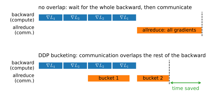
- No overlap. Our loop finished the entire backward pass, then called
allreduce. But gradients become available layer by layer, back to front, so the last layers’ gradients could be communicated while the earlier layers are still computing. Serializing compute-then-communicate wastes exactly the time the fabric is idle during backward. - One Python process. A single interpreter drove all \(k\) GPUs, so one GIL-bound thread dispatched every kernel — the overhead regime of Section 13.1, multiplied by \(k\).
- A star topology. Our
allreducerouted every transfer through device 0; Section 13.5.3 showed the ring moves a constant per device instead.
PyTorch’s DistributedDataParallel (DDP) fixes all three (Li et al. 2020): one process per GPU (no shared GIL), NCCL’s ring/tree collectives (no hub), and — the headline — gradient bucketing that overlaps communication with the backward pass (Figure 13.6.1). As each bucket of gradients fills, DDP kicks off its allreduce immediately, so by the time the backward pass reaches the first layer, the last layers’ gradients are already summed. This is compute–communication overlap — independent work scheduled onto the fabric while the GPUs keep computing — finally shown where it pays.
13.6.2 Distributed Data Parallel
DDP needs multiple processes, and a notebook is one process — so we launch the extra ones. The idiom, verified to work under this book’s build: write the training script to a sidecar file, then launch it with torchrun, which spawns one process per GPU, sets up the rendezvous, and runs the script under init_process_group. Each rank writes its result to a scratch directory the notebook reads back (cleared before every launch, so a crashed run can never serve stale numbers). We keep the script minimal; the loop body is unchanged from single-GPU training, and the scaffolding around it is what the launcher’s multi-process world requires:
def resnet18(num_classes, in_channels=1):
    """A slightly modified ResNet-18 model."""
    def resnet_block(in_channels, out_channels, num_residuals,
                     first_block=False):
        blk = []
        for i in range(num_residuals):
            if i == 0 and not first_block:
                blk.append(d2l.Residual(out_channels, use_1x1conv=True,
                                        strides=2))
            else:
                blk.append(d2l.Residual(out_channels))
        return nn.Sequential(*blk)

    # This model uses a smaller convolution kernel, stride, and padding and
    # removes the max-pooling layer
    net = nn.Sequential(
        nn.Conv2d(in_channels, 64, kernel_size=3, stride=1, padding=1),
        nn.BatchNorm2d(64),
        nn.ReLU())
    net.add_module("resnet_block1", resnet_block(64, 64, 2, first_block=True))
    net.add_module("resnet_block2", resnet_block(64, 128, 2))
    net.add_module("resnet_block3", resnet_block(128, 256, 2))
    net.add_module("resnet_block4", resnet_block(256, 512, 2))
    net.add_module("global_avg_pool", nn.AdaptiveAvgPool2d((1,1)))
    net.add_module("fc", nn.Sequential(nn.Flatten(),
                                       nn.Linear(512, num_classes)))
    return net
class ResNet18(nnx.Module):
    """A slightly modified ResNet-18 (small stem, no max-pool)."""
    def __init__(self, num_classes=10, rngs=None):
        rngs = nnx.Rngs(d2l.get_key()) if rngs is None else rngs
        self.net = nnx.Sequential(
            nnx.Conv(1, 64, (3, 3), (1, 1), padding='same', rngs=rngs),
            nnx.BatchNorm(64, rngs=rngs), nnx.relu,
            d2l.Residual(64, in_channels=64, rngs=rngs),
            d2l.Residual(64, in_channels=64, rngs=rngs),
            d2l.Residual(128, use_1x1conv=True, strides=(2, 2),
                         in_channels=64, rngs=rngs),
            d2l.Residual(128, in_channels=128, rngs=rngs),
            d2l.Residual(256, use_1x1conv=True, strides=(2, 2),
                         in_channels=128, rngs=rngs),
            d2l.Residual(256, in_channels=256, rngs=rngs),
            d2l.Residual(512, use_1x1conv=True, strides=(2, 2),
                         in_channels=256, rngs=rngs),
            d2l.Residual(512, in_channels=512, rngs=rngs),
            lambda x: x.mean(axis=(1, 2)),
            nnx.Linear(512, num_classes, rngs=rngs))

    def __call__(self, x):
        return self.net(x)
The DDP training script, written to disk from a cell. The two lines that make training data-parallel are init_process_group("nccl") once per process and the DDP(model) wrap — after those, the loop body is unchanged from single-GPU. The remaining code implements the launcher’s required process setup: a rank-local device, a DistributedSampler that hands each rank a disjoint shard of the data (re-shuffled per epoch by set_epoch), and process-group teardown. The parent notebook downloads Fashion-MNIST once, quietly, before any rank exists, so the ranks never race on the download:
with contextlib.redirect_stdout(io.StringIO()), \
     contextlib.redirect_stderr(io.StringIO()):     # download once, quietly
    datasets.FashionMNIST('./data', train=True, download=True)

DDP_SCRIPT = r'''
import json, os, sys, time, torch
from torch import nn
import torch.distributed as dist
from torch.nn.parallel import DistributedDataParallel as DDP
from torchvision import datasets, transforms
from d2l import torch as d2l

rank = int(os.environ["LOCAL_RANK"]); world = int(os.environ["WORLD_SIZE"])
torch.cuda.set_device(rank); dist.init_process_group("nccl")
torch.set_float32_matmul_precision("high"); torch.backends.cudnn.benchmark = True

model = d2l.resnet18(10, 1).to(rank)
model(torch.zeros(1, 1, 64, 64, device=rank))     # materialize Lazy params
model = DDP(model, device_ids=[rank])
opt = torch.optim.SGD(model.parameters(), lr=0.1)
loss = nn.CrossEntropyLoss()

B = int(sys.argv[1]) if len(sys.argv) > 1 else 256   # per-rank batch size
tf = transforms.Compose([transforms.Resize(64), transforms.ToTensor()])
ds = datasets.FashionMNIST("./data", train=True, transform=tf)
sampler = torch.utils.data.distributed.DistributedSampler(ds, world, rank)
loader = torch.utils.data.DataLoader(ds, B, sampler=sampler, num_workers=2)

for epoch in range(2):                             # epoch 0 warms up
    sampler.set_epoch(epoch); n = 0; torch.cuda.synchronize(); t0 = time.time()
    for X, y in loader:
        X, y = X.to(rank), y.to(rank)
        opt.zero_grad(set_to_none=True)
        loss(model(X), y).backward(); opt.step(); n += X.shape[0]
    torch.cuda.synchronize(); dt = time.time() - t0
here = os.path.dirname(os.path.abspath(__file__))
with open(os.path.join(here, f"rank{rank}.json"), "w") as f:
    json.dump({"rank": rank, "samples_per_s": n / dt}, f)
dist.destroy_process_group()
'''
DDP_DIR = pathlib.Path('ddp_scratch')
DDP_DIR.mkdir(exist_ok=True)
_ = (DDP_DIR / 'train_ddp.py').write_text(DDP_SCRIPT)
One word before the numbers, because every published speedup quietly picks a convention (Section 13.5.4). This sweep holds the per-rank batch fixed at 256, so the global batch grows to \(256k\) — weak scaling: the efficiencies it prints are throughput per GPU relative to one GPU. Remember that a grown global batch also changes the optimization trajectory itself (Section 9.10); the strong-scaling question — same global batch, finishing sooner — comes right after.
def ddp_throughput(k, batch_size=256):
    """Launch k-process DDP via torchrun; return aggregate samples/s."""
    for stale in DDP_DIR.glob('rank*.json'):   # a crashed run must not
        stale.unlink()                         # serve old results
    torchrun = str(pathlib.Path(sys.executable).parent / 'torchrun')
    subprocess.run([torchrun, '--standalone', f'--nproc-per-node={k}',
                    str(DDP_DIR / 'train_ddp.py'), str(batch_size)],
                   check=True)
    per_rank = []
    for r in range(k):
        with open(DDP_DIR / f'rank{r}.json') as f:
            per_rank.append(json.load(f)['samples_per_s'])
    return sum(per_rank)

ks = [k for k in (1, 2, 4) if k <= d2l.num_gpus()]
tput = [ddp_throughput(k) for k in ks]
for k, t in zip(ks, tput):
    print(f'{k} GPU(s): {t:.0f} samples/s, {t / tput[0]:.2f}x, '
          f'{100 * t / tput[0] / k:.0f}% weak-scaling efficiency')
d2l.plot(ks, [tput], 'GPUs', 'samples/s')
1 GPU(s): 2107 samples/s, 1.00x, 100% weak-scaling efficiency
2 GPU(s): 3714 samples/s, 1.76x, 88% weak-scaling efficiency
4 GPU(s): 6924 samples/s, 3.29x, 82% weak-scaling efficiency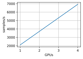
On our four-GPU box, ResNet-18 on Fashion-MNIST-64 (11.2M parameters) scales the way the accounting of Section 13.5 says a compute-dense model should: about 1.8× at two GPUs and about 3.3× at four — the cell prints 88% and 82% weak-scaling efficiency. The efficiency sags gently — no cliff — because each step’s compute is large enough to hide most of the communication, unlike LeNet. Strong scaling asks a harder question of the same hardware: hold the global batch at 512 and split it ever thinner, so the per-rank batch shrinks as \(512/k\) while the allreduce stays the same size:
tput_strong = [ddp_throughput(k, batch_size=512 // k) for k in ks]
for k, t in zip(ks, tput_strong):
    print(f'{k} GPU(s): {t:.0f} samples/s, {t / tput_strong[0]:.2f}x, '
          f'{100 * t / tput_strong[0] / k:.0f}% strong-scaling efficiency')
d2l.plot(ks, [tput, tput_strong], 'GPUs', 'samples/s',
         legend=['weak (per-rank 256)', 'strong (global 512)'])
1 GPU(s): 2092 samples/s, 1.00x, 100% strong-scaling efficiency
2 GPU(s): 3717 samples/s, 1.78x, 89% strong-scaling efficiency
4 GPU(s): 5885 samples/s, 2.81x, 70% strong-scaling efficiency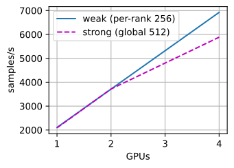
At two GPUs the two conventions nearly coincide on this model — a 4090 is about equally saturated by a per-rank batch of 256 or 512, so the \(k=1\) baselines barely differ — but they part company as \(k\) grows: by \(k=4\) the strong-scaling run gives each GPU only 128 examples per step, and any gap that opens between the strong and weak efficiencies is pure underutilization, the mechanism that sank LeNet, now in miniature. That is Equation 13.5.2 read twice: weak scaling holds \(t_{\text{compute}}\) per device constant and asks the fabric to keep up; strong scaling shrinks \(t_{\text{compute}}(B/k)\) toward the fixed \(t_{\text{comm}}\) floor.
Now confront the sweep with the cost model by measurement rather than by assertion. Equation 13.5.2 prices a step’s communication at \(2N/\beta\), and DDP itself provides the instrument to check it: no_sync() runs backward with gradient synchronization turned off, so the difference between synced and unsynced step times estimates what communication really costs — an estimate, not a truth, since turning sync off also changes what overlaps what:
COMM_SCRIPT = r'''
import contextlib, json, os, time, torch
from torch import nn
import torch.distributed as dist
from torch.nn.parallel import DistributedDataParallel as DDP
from d2l import torch as d2l

rank = int(os.environ["LOCAL_RANK"])
torch.cuda.set_device(rank)
dist.init_process_group("nccl", device_id=torch.device("cuda", rank))
torch.set_float32_matmul_precision("high"); torch.backends.cudnn.benchmark = True

model = d2l.resnet18(10, 1).to(rank)
model(torch.zeros(1, 1, 64, 64, device=rank))
model = DDP(model, device_ids=[rank])
loss = nn.CrossEntropyLoss()
X = torch.randn(256, 1, 64, 64, device=rank)
y = torch.randint(0, 10, (256,), device=rank)

def fwd_bwd():
    model.zero_grad(set_to_none=True)
    loss(model(X), y).backward()

def step_time(sync_grads, steps=30):
    ctx = contextlib.nullcontext if sync_grads else model.no_sync
    for _ in range(10):                            # warmup
        with ctx(): fwd_bwd()
    torch.cuda.synchronize(); dist.barrier(); t0 = time.time()
    for _ in range(steps):
        with ctx(): fwd_bwd()
    torch.cuda.synchronize()
    return (time.time() - t0) / steps

synced, silent = step_time(True), step_time(False)
if rank == 0:
    here = os.path.dirname(os.path.abspath(__file__))
    with open(os.path.join(here, "comm.json"), "w") as f:
        json.dump({"synced_ms": 1e3 * synced, "no_sync_ms": 1e3 * silent}, f)
dist.destroy_process_group()
'''
_ = (DDP_DIR / 'comm_probe.py').write_text(COMM_SCRIPT)

net = resnet18(10, 1)                     # the gradient bytes, N
net(torch.zeros(1, 1, 64, 64))            # materialize Lazy params
n_bytes = 4 * sum(p.numel() for p in net.parameters())
beta = 4.5e9   # NCCL allreduce, effective bytes/device/s on this box (13.5)
if d2l.num_gpus() >= 2:
    torchrun = str(pathlib.Path(sys.executable).parent / 'torchrun')
    subprocess.run([torchrun, '--standalone', '--nproc-per-node=2',
                    str(DDP_DIR / 'comm_probe.py')], check=True)
    with open(DDP_DIR / 'comm.json') as f:
        comm = json.load(f)
    print(f"k=2: predicted comm 2N/beta = {2 * n_bytes / beta * 1e3:.0f} "
          f"ms/step; measured {comm['synced_ms'] - comm['no_sync_ms']:.0f} ms "
          f"(synced {comm['synced_ms']:.0f}, no_sync {comm['no_sync_ms']:.0f})")
k=2: predicted comm 2N/beta = 20 ms/step; measured 15 ms (synced 132, no_sync 117)Prediction and measurement are within tens of percent in this setup. This agreement supports using Equation 13.5.2 for the tested message sizes and topology; it is not a hardware-independent scaling guarantee. An NVLink fabric shrinks \(t_{\text{comm}}\) by roughly two orders of magnitude (Table 13.2.1), so the same accounting predicts near-linear scaling — same model, different constant. (The legacy nn.DataParallel is single-process and GIL-bound; use DDP even on one node, as PyTorch’s own docs advise.)
The following measurement tests one diagnosis from Section 13.5: that NCCL’s P2P-less fallback moves bytes with a latency-bound GPU-kernel copy — in effect a performance bug in how the library’s default transport interacts with this particular platform — and that one documented switch, NCCL_SHM_USE_CUDA_MEMCPY=1, re-routes the same transfer over the DMA copy engines. Measure the bare collective both ways:
BENCH_SCRIPT = r'''
import json, os, time, torch
import torch.distributed as dist

rank = int(os.environ["LOCAL_RANK"])
torch.cuda.set_device(rank)
dist.init_process_group("nccl", device_id=torch.device("cuda", rank))
x = torch.randn(16 * 1024 * 1024, device=rank)     # 64 MB of fp32
for _ in range(5):                                 # warmup
    dist.all_reduce(x)
torch.cuda.synchronize(); t0 = time.time()
for _ in range(15):
    dist.all_reduce(x)
torch.cuda.synchronize(); dt = (time.time() - t0) / 15
if rank == 0:
    here = os.path.dirname(os.path.abspath(__file__))
    with open(os.path.join(here, "bench.json"), "w") as f:
        json.dump({"gbs": 2 * x.numel() * 4 / dt / 1e9}, f)
dist.destroy_process_group()
'''
_ = (DDP_DIR / 'allreduce_bench.py').write_text(BENCH_SCRIPT)

def bare_allreduce_gbs(**env):
    (DDP_DIR / 'bench.json').unlink(missing_ok=True)
    torchrun = str(pathlib.Path(sys.executable).parent / 'torchrun')
    subprocess.run([torchrun, '--standalone', '--nproc-per-node=2',
                    str(DDP_DIR / 'allreduce_bench.py')],
                   check=True, env={**os.environ, **env})
    with open(DDP_DIR / 'bench.json') as f:
        return json.load(f)['gbs']

if d2l.num_gpus() >= 2:
    slow = bare_allreduce_gbs()
    # Works around an NCCL transport bottleneck on this P2P-less box
    # (13.5's diagnosis) -- a platform-specific fix; validate on yours.
    fast = bare_allreduce_gbs(NCCL_SHM_USE_CUDA_MEMCPY='1')
    print(f'bare allreduce, effective bytes/device/s: '
          f'{slow:.1f} GB/s at the default, {fast:.1f} GB/s configured '
          f'({fast / slow:.1f}x)')
bare allreduce, effective bytes/device/s: 4.4 GB/s at the default, 22.3 GB/s configured (5.1x)This configuration changes effective bandwidth by roughly a factor of five. The collective transport and its assumed topology can therefore change communication performance substantially, so measure yours against what the wire demonstrably carries (Section 13.5’s raw copy) before trusting it. Then the specific one, which is why every training run above still uses the library’s defaults: this workaround improves the microbenchmark but deadlocks the training workload. On our box, with this NCCL build, the copy-engine mode deadlocks DDP’s overlapped training path within seconds — the very collectives that just ran flawlessly in isolation wedge inside the training loop — so adopting it here would trade a five-fold bandwidth win for a hung notebook. The workaround is specific to both the platform and the workload: measure whether it is needed and whether training remains reliable (the exercises reproduce both cases). Equation Equation 13.5.2 uses the measured \(\beta\) of the configured fabric in either case.
13.6.3 Fully Sharded Data Parallelism
DDP replicates the parameters, gradients, and optimizer states on every rank. For the \(16P\)-byte training footprint of Section 13.4, this creates \(k-1\) redundant copies and limits the model to the capacity of one GPU, the limitation Section 13.5 flagged. Fully Sharded Data Parallel (FSDP) removes the redundancy by sharding those tensors across ranks, each rank owning \(1/k\) of each, and materializing a full layer only for the moment it is needed (Zhao et al. 2023). The idea is the ZeRO sequence (Rajbhandari et al. 2020): shard the optimizer states first (they are the biggest, \(8P\)), then the gradients, then the parameters. Each stage reduces replicated memory toward \(1/k\) while introducing additional communication.
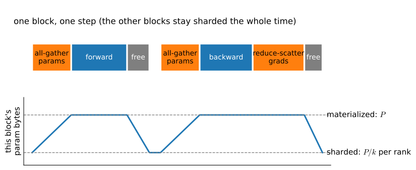
The mechanism follows the collective identity in Section 13.5. Allreduce equals reduce-scatter followed by all-gather. FSDP keeps these two phases separate: an all-gather reconstructs a layer’s full parameters just before it computes, and frees them just after; a reduce-scatter sums each layer’s gradients but leaves each rank holding only its own shard (Figure 13.6.2). No tensor’s full replica ever lives longer than the layer that needs it.
The following table summarizes the collectives used in the remainder of the book:
| collective | what every rank ends with | where it appears |
|---|---|---|
| allreduce | the full sum | DDP’s gradient buckets; Section 13.5 |
| reduce-scatter | one shard of the sum | FSDP gradients |
| all-gather | every shard, concatenated | FSDP parameters, just-in-time |
| all-to-all | a different shard from each peer | expert parallelism (Section 30.6) |
FSDP is useful when replicated training state does not fit on one device. That benefit is not measurable on our 11.2M-parameter demo, which occupies a few hundred MB of a 24 GB card, so we show the shape of the code rather than run it. The modern API is fully_shard over a DeviceMesh; the original FullyShardedDataParallel wrapper class still imports at our pin, but it is the deprecated legacy path:
# Code sketch (not executed): shard each block, then the whole model.
# from torch.distributed.fsdp import fully_shard
# from torch.distributed.device_mesh import init_device_mesh
# mesh = init_device_mesh("cuda", (world_size,))
# model = build_large_model()
# for block in model.transformer_blocks:   # shard per repeated block
#     fully_shard(block, mesh=mesh)
# fully_shard(model, mesh=mesh)            # shard the remainder
print('FSDP sketch: reach for it past a few billion parameters, '
      'not on an 11M-param demo')
FSDP sketch: reach for it past a few billion parameters, not on an 11M-param demo# In JAX the same sharding is a PartitionSpec, not a wrapper — see below.
print('JAX shards by annotation; the next subsection is the demo')JAX shards by annotation; the next subsection is the demoYou reach for FSDP when the training state at your precision no longer fits on one GPU — the parameters, gradients, and optimizer states of Section 13.4’s anatomy, plus activations — or when that redundancy is worth trading away for communication; for this card class the threshold arrives at a few billion parameters. The production distributed-training map, and how to combine FSDP with the other parallelism axes, lives in Section 30.6.
13.6.4 Declarative Sharding in JAX
The PyTorch implementation uses multiple processes, explicit collectives, and a launcher. JAX instead expresses sharding in one process over all available GPUs. One process sees all the GPUs (Section 13.2.5); you describe how the data is laid out across them with a Mesh and a NamedSharding, device_put the arrays onto that layout — parameters replicated (P()), the batch sharded along its leading axis (P('data')) — and jit the unchanged single-device training step. XLA’s automatic-parallelization pass (GSPMD (Xu et al. 2021)) partitions the computation to match the data layout and inserts the very allreduce that Section 13.5 wrote by hand — you never write a collective:
def make_mesh(k):
    return jax.make_mesh((k,), ('data',))

def shard_batch(X, y, mesh):
    P = jax.sharding.PartitionSpec('data')      # leading axis across devices
    sh = jax.sharding.NamedSharding(mesh, P)
    return jax.device_put(X, sh), jax.device_put(y, sh)

def replicate(module, mesh):
    """Give every device of the mesh a full copy of a module's state."""
    sh = jax.sharding.NamedSharding(mesh, jax.sharding.PartitionSpec())
    nnx.update(module, jax.device_put(nnx.state(module), sh))

# The training step is written for one device; jit + sharded inputs make it
# data-parallel with no change to the body.
@nnx.jit
def train_step(model, opt, X, y):
    def loss_fn(m):
        return optax.softmax_cross_entropy_with_integer_labels(
            m(X), y).mean()
    loss, grads = nnx.value_and_grad(loss_fn)(model)
    opt.update(model, grads)                     # XLA inserts the allreduce
    return loss
We run the example with ResNet18, an optimizer, and a Fashion-MNIST batch resized once to 64×64 and retained as host arrays. visualize_array_sharding displays where each tensor resides: the batch split across the mesh before the step, and a weight after the step still replicated everywhere — the compiler’s allreduce is what kept every copy identical:
imgs, labels = d2l.FashionMNIST().train         # raw arrays; resize once
X_all = np.asarray(jax.image.resize(
    jnp.float32(imgs[:, :, :, None]) / 255, (len(imgs), 64, 64, 1),
    'bilinear'))
y_all = np.asarray(labels, np.int32)

k = min(4, jax.local_device_count())
mesh = make_mesh(k)
model = ResNet18(rngs=nnx.Rngs(0))
opt = nnx.Optimizer(model, optax.sgd(0.1), wrt=nnx.Param)
replicate(model, mesh); replicate(opt, mesh)
Xs, ys = shard_batch(X_all[:256], y_all[:256], mesh)
loss = train_step(model, opt, Xs, ys)           # one data-parallel step
print(f'one sharded step: loss {float(loss):.2f}')
print('the batch, split along its leading axis:')
jax.debug.visualize_array_sharding(Xs.reshape(len(Xs), -1))
print('a weight after the step, still replicated:')
jax.debug.visualize_array_sharding(model.net.layers[-1].kernel[...])
one sharded step: loss 2.47
the batch, split along its leading axis:
┌──────────────────────────────────────────────────────────────────────────────┐
│ GPU 0 │
├──────────────────────────────────────────────────────────────────────────────┤
│ GPU 1 │
├──────────────────────────────────────────────────────────────────────────────┤
│ GPU 2 │
├──────────────────────────────────────────────────────────────────────────────┤
│ GPU 3 │
└──────────────────────────────────────────────────────────────────────────────┘
a weight after the step, still replicated:
┌───────────┐
│ │
│ │
│ │
│ │
│GPU 0,1,2,3│
│ │
│ │
│ │
│ │
└───────────┘Take the receipt. Section 13.5 wrote its pmean by hand; here nobody wrote a collective — so where is it? In the compiled program. Lower and compile the step, and search the XLA text for what GSPMD inserted:
hlo = train_step.lower(model, opt, Xs, ys).compile().as_text()
ops = [line.strip() for line in hlo.splitlines()
       if ' all-reduce(' in line or ' all-reduce-start(' in line]
sizes = [int(re.search(r'\[(\d+)\]', op).group(1)) for op in ops]
print(f'{len(ops)} all-reduce ops in the compiled step; the largest '
      f'sums {max(sizes) / 1e6:.1f}M floats:')
print(ops[sizes.index(max(sizes))][:88] + ' ...')
36 all-reduce ops in the compiled step; the largest sums 6.4M floats:
%all-reduce-start.34 = f32[6447680]{0} all-reduce-start(%wrapped_concatenate.34), channe ...Dozens of allreduces, not one — and reading them teaches. The two largest together carry the ~11M gradient floats (XLA bucketed them into two fused sums, much as DDP buckets); the many small ones are batch-norm statistics, because under jit even normalization is computed over the global batch — the compiler preserves single-device semantics exactly, where DDP leaves each replica its own batch-norm statistics unless you ask for SyncBatchNorm. (The exact count depends on compilation; the two largest collectives dominate communication.)
Measured, under the same weak-scaling convention as the DDP sweep (per-device batch 256) — one process, no launcher, no sidecar files:
def batches(global_batch):
    n = (len(X_all) // global_batch) * global_batch
    for i in range(0, n, global_batch):
        yield X_all[i:i + global_batch], y_all[i:i + global_batch]

def jax_throughput(k, per_device_batch=256):
    mesh = make_mesh(k)
    model = ResNet18(rngs=nnx.Rngs(0))
    opt = nnx.Optimizer(model, optax.sgd(0.1), wrt=nnx.Param)
    replicate(model, mesh); replicate(opt, mesh)
    B = per_device_batch * k
    for epoch in range(2):                 # epoch 0 warms up and compiles
        t0 = time.time(); n = 0
        for X, y in batches(B):
            loss = train_step(model, opt, *shard_batch(X, y, mesh))
            n += X.shape[0]
        loss.block_until_ready()           # completion timing
        dt = time.time() - t0
    return n / dt

ks = [k for k in (1, 2, 4) if k <= jax.local_device_count()]
tput = [jax_throughput(k) for k in ks]
for k, t in zip(ks, tput):
    print(f'{k} GPU(s): {t:.0f} samples/s, {t / tput[0]:.2f}x, '
          f'{100 * t / tput[0] / k:.0f}% weak-scaling efficiency')
1 GPU(s): 2669 samples/s, 1.00x, 100% weak-scaling efficiency
2 GPU(s): 4388 samples/s, 1.64x, 82% weak-scaling efficiency
4 GPU(s): 8010 samples/s, 3.00x, 75% weak-scaling efficiencyThe shape matches the DDP sweep — real gains, efficiency sagging as \(k\) grows, no cliff — with one instructive difference: the compiled XLA step is faster per device, so the same allreduce is a larger fraction of each step and the efficiency reads a few points lower (82% already at two GPUs in our runs). That is Equation 13.5.2 again: speed up the compute and the fabric gets relatively slower. These measurements are not this loop feeds pre-staged host arrays while the DDP script pays a real DataLoader, so the absolute samples/s are not a framework shoot-out — the scaling curve is the comparison.
One more check, because we are trusting a collective nobody wrote. Section 13.5 ended its hand-built loop with a one-step equality test, and the declarative version deserves the same scrutiny — same initialization, same 256-example batch, one step on one device versus one step sharded across two:
def one_step_delta(k):
    mesh = make_mesh(k)
    model = ResNet18(rngs=nnx.Rngs(0))
    opt = nnx.Optimizer(model, optax.sgd(0.1), wrt=nnx.Param)
    replicate(model, mesh); replicate(opt, mesh)
    before = jax.tree.map(np.asarray, nnx.state(model, nnx.Param))
    train_step(model, opt, *shard_batch(X_all[:256], y_all[:256], mesh))
    after = jax.tree.map(np.asarray, nnx.state(model, nnx.Param))
    return jax.tree.map(lambda a, b: a - b, after, before)

d1 = one_step_delta(1)
d2 = one_step_delta(min(2, jax.local_device_count()))
gaps = jax.tree.map(lambda a, b: np.abs(a - b).max(), d1, d2)
print('max update difference, k=1 vs k=2: '
      f'{max(jax.tree.leaves(gaps)):.1e}')
max update difference, k=1 vs k=2: 1.5e-04The two runs agree to about \(10^{-4}\) against update magnitudes near \(10^{-2}\) — not the \(10^{-9}\) of Section 13.5’s LeNet check, and the gap is itself informative: these are two different compiled programs, whose tf32 convolutions and batch-norm reductions associate their arithmetic differently, so the residue is rounding. What the check exists to catch would announce itself at the scale of the update itself: a summed-instead-of-averaged gradient, an accidental \(k\times\) learning rate.
In JAX, moving between data parallelism, tensor parallelism, and FSDP-style sharding in JAX, you change the PartitionSpec — not the model code. Sharding the batch axis gives data parallelism (above); sharding a weight’s feature axis gives tensor parallelism; sharding the parameters and letting XLA all-gather them just-in-time gives the FSDP pattern. One sharding vocabulary spans what PyTorch exposes as three different APIs (DDP, tensor-parallel wrappers, FSDP): annotate the layout, and the compiler writes the collectives. An effective sharding plan is still model-aware, though: someone has to choose the layouts and the constraint points. The manual end of the same spectrum is the jax.shard_map + lax.psum of Section 13.5, where you write the collective yourself; jit + sharding is the automatic end.
| PyTorch | JAX | |
|---|---|---|
| processes | one per GPU (torchrun) |
one, sees all GPUs |
| collectives | explicit (NCCL, or DDP’s buckets) | inserted by XLA/GSPMD |
| data parallel | DistributedDataParallel |
shard the batch axis |
| tensor parallel | separate wrappers / DTensor | change the PartitionSpec |
| sharded (FSDP) | fully_shard |
change the PartitionSpec |
| control | imperative, visible | declarative, compiler-driven |
Neither deal is strictly better: PyTorch’s explicitness makes the communication legible and debuggable; JAX’s declarativeness makes the same code span parallelism strategies by editing an annotation. Knowing both is knowing the design space.
13.6.5 When One Node Is Not Enough
This chapter considers a single machine. Larger systems add further forms of parallelism. When a model is too large for even sharded data parallelism on one node — when the parameters, or the batch, or the sequence length outgrow what \(k\) local GPUs can hold — the answer is to shard across machines, combining data parallelism with tensor, pipeline, and expert parallelism into the “3D parallelism” of frontier training. The collectives then run over a network fabric measured in tens of GB/s between nodes rather than an NVLink domain within one, and the cost model of Section 13.5 acquires a second, slower bandwidth term. That is the province of the Language Models part, which has models and datasets large enough to warrant it; the production library map is Section 30.6 — Megatron, the FSDP/DTensor stack, DeepSpeed, and how to launch and checkpoint them across a cluster. From here the communication algebra stays the same; what multi-node adds is engineering on top of it — a hierarchy of fabrics (NVLink inside a node, a network between nodes), rendezvous and elastic restart when machines fail, and stragglers that turn a synchronous step into a queueing problem.
13.6.6 Summary
- Production data parallelism (DDP) fixes the three deficits of a hand-rolled loop: one process per GPU (no shared GIL), ring/tree collectives (no hub), and gradient bucketing that overlaps communication with the backward pass.
- Launched from a notebook via
torchrunon a sidecar script, DDP scales a compute-dense ResNet-18 by roughly 1.8× on two GPUs and 3.3× on four on our host-staged box (88% and 82% weak-scaling efficiency; a fixed-global-batch strong-scaling sweep asks the harder question), and ano_sync()measurement confirms Equation 13.5.2’s communication price to within tens of percent. An NVLink box changes only the constant. - The constant is also configuration-sensitive: one documented NCCL switch quintuples the bare-collective bandwidth on this box — yet deadlocks DDP’s overlapped training path, so the notebooks keep the library’s defaults and teach the pair of measurements instead. Collective-library configuration moves communication by factors, not percent; a workaround is validated per platform and per workload.
- FSDP shards the \(16P\)-byte training state across ranks in successive ZeRO stages by splitting allreduce back into its reduce-scatter and all-gather halves and materializing each layer just-in-time. It is for models whose training state outgrows one GPU — a few billion parameters on this card class.
- JAX inverts the model: one process, annotate the data layout with a
MeshandPartitionSpec,jitthe unchanged step, and XLA inserts the collectives — visible in the compiled program’sall-reduceops, measured in a k-sweep, and verified by a k=1-versus-k=2 equality check. Changing thePartitionSpec— not the code — moves between data, tensor, and FSDP-style sharding, spanning what PyTorch exposes as three APIs. - Multi-node 3D parallelism and the production library map are the Language Models part and Section 30.6.
13.6.7 Exercises
- Weak-scaling extrapolation. The DDP sweep of Section 13.6.2 reports weak-scaling efficiencies of 88% at \(k = 2\) and 82% at \(k = 4\). Suppose that a step on \(k\) GPUs takes the single-GPU step time \(t_1\) plus an exposed communication time, and that this exposed time is proportional to the per-device ring traffic of
Equation 13.5.1.
- Express the efficiency \(E(k)\) through a single constant, fit the constant to the measurement at \(k = 2\), and predict \(E(4)\). Compare your prediction with the measured 82% and with the prediction of a model in which the exposed time is the same for every \(k \geq 2\).
- Predict \(E(8)\) for an eight-GPU machine of the same design as the four-GPU build machine, on which every inter-GPU transfer is staged through host memory (Section 13.2.5). How does the total ring traffic through host memory grow with \(k\), and in which direction should this move a measured \(E(8)\) relative to your prediction?
- With gradient accumulation (Section 13.4.5), each rank runs \(a\) micro-batches of 256 examples per optimizer step and synchronizes only after the last one. Starting from the measured 82%, find the smallest \(a\) that raises the efficiency at \(k = 4\) to 95%. What happens to the global batch, and why does that matter (Section 9.10)?
- Strong versus weak efficiency. Model the forward and backward time of one device at per-device batch \(b\) as \(t_{\text{compute}}(b) = t_0 + c\,b\), where \(t_0\) is a fixed cost per step that does not shrink with the batch and \(c\) is the time per example. Let the communication of a step on \(k > 1\) devices take \((1 - 1/k)\,\tau\) with \(\tau = 2N/\beta\), the ring traffic of Equation 13.5.1 at the bandwidth of Equation 13.5.2, without overlap. Let \(E_{\text{weak}}(k; b)\) be the weak-scaling efficiency at per-device batch \(b\), and \(E_{\text{strong}}(k)\) the strong-scaling efficiency at global batch \(B\).
Show that
\[E_{\text{strong}}(k) = E_{\text{weak}}(k; B/k)\, \frac{t_0 + c B}{k\, t_0 + c B}. \tag{13.6.1}\]
What does this identity say about the gap between the weak and the strong sweeps of Section 13.6.2 at equal per-device batch?
Section 13.6.2 reports that an RTX 4090 is about equally saturated by per-rank batches of 256 and 512 for ResNet-18. What does that say about \(t_0\) for this model? For the LeNet of Section 13.5, \(t_{\text{compute}}(B/2) \approx t_{\text{compute}}(B)\); what bound does the identity then place on \(E_{\text{strong}}(2)\)?
- ZeRO memory budget. A model with 7 billion parameters is to be trained with Adam on 8 GPUs with 80 GB each. Use the anatomy of Section 13.4.1 (16 bytes per parameter before activations) and ignore activations. ZeRO (Rajbhandari et al. 2020) shards the optimizer states across the GPUs in stage 1, also the gradients in stage 2, and also the parameters in stage 3 (Section 13.6.3).
- Compute the per-GPU training state under DDP and under each of the three stages. Which configurations fit, and how much memory does each leave for activations?
- For each configuration, find the largest model whose training state fits on these 8 GPUs. How does this limit grow as more GPUs join, and what caps it for DDP and for stages 1 and 2?
- Cost of sharding. Count the communication per device and step in units of \(N\), the bytes of one full set of gradients, and assume that parameters are communicated in the same precision, so that a full set of parameters also occupies \(N\) bytes. With the ring algorithm of Section 13.5.3, an allreduce moves \(2(k-1)N/k\) bytes per device, and each of its two phases, a reduce-scatter and an all-gather, moves \((k-1)N/k\).
- In ZeRO stages 1 and 2 (Rajbhandari et al. 2020), each rank updates only its own shard of the parameters, and every rank needs the full parameters again before the next forward pass. Name the collectives that one step of each stage needs, and compare their volume with the allreduce of DDP.
- In stage 3, the FSDP lifecycle of Figure 13.6.2 gathers each block’s parameters for its forward pass, frees them, and gathers them again for its backward pass. Count the collectives of one step and compare their volume with DDP.
- A variant keeps every gathered block from its forward pass until its backward pass. Which collective does this remove, and how much of the memory saving of stage 3 does it give up, in terms of the 16-byte anatomy of Section 13.4.1?
- [code] Splitting the data.
train_ddp.pygives each rank a disjoint shard of Fashion-MNIST through aDistributedSamplerand reshuffles the shards every epoch withsampler.set_epoch.- Remove the sampler, so that every rank builds the same
DataLoaderover the full dataset. Predict, for \(k = 2\), the aggregate throughput thatddp_throughputreports relative to the correct script, the time an epoch takes, and the global batch that the averaged gradient corresponds to. Then run it, with each rank printing a checksum of its first batch. - Restore the sampler and remove only the call to
set_epoch. What changes from one epoch to the next, and what stays the same? - Name a check that catches both mistakes and is cheap enough to run on every launch.
- Remove the sampler, so that every rank builds the same
- [code] Splitting the data.
shard_batchplaces the batch withPartitionSpec('data'), which splits its leading axis across the mesh.- Change
shard_batchto place the batch withPartitionSpec(), which replicates it on every device. Predict which collectives the compiledtrain_stepcontains and how the throughput ofjax_throughput(2)compares with that ofjax_throughput(1), then check both. - Place the images with
PartitionSpec(None, 'data'), which splits the height of every image across the devices, and keep the labels replicated. Which values must neighboring devices exchange for a \(3 \times 3\) convolution, and which collective does that take? Find it in the compiledtrain_step.
- Change