import torch1.5 Automatic Differentiation
Recall from Section 1.4 that derivatives drive all the optimization algorithms that we will use to train deep networks. Even when the individual rules are elementary, applying them by hand becomes tedious and error-prone as models grow more complex.
Modern deep learning frameworks perform this calculation using automatic differentiation (often shortened to autograd). As we pass data through each successive function, the framework builds a computational graph that tracks how each value depends on others. To calculate derivatives, automatic differentiation works backwards through this graph applying the chain rule. The computational algorithm for applying the chain rule in this fashion is called backpropagation.
Autograd has a long history: the earliest references date back over half a century (Wengert 1964), and reverse mode, the variant that powers modern backpropagation, was developed by Linnainmaa (1970) . Section 25.3 recounts this history in full. We begin with the basic automatic-differentiation interface and then examine how computational graphs are controlled.
import tensorflow as tffrom jax import numpy as jnpfrom mxnet import autograd, np, npx
npx.set_np()1.5.1 Mechanics
We begin with the basic workflow (attach a gradient, record a computation, run the backward pass), first on a scalar-valued function, then on vector-valued ones.
1.5.1.1 A Simple Function
Consider differentiating the function \(y = 2\mathbf{x}^{\top}\mathbf{x}\) with respect to the column vector \(\mathbf{x}\). To start, we assign x an initial value.
x = torch.arange(4.0)
x
tensor([0., 1., 2., 3.])x = tf.range(4, dtype=tf.float32)
x<tf.Tensor: shape=(4,), dtype=float32, numpy=array([0., 1., 2., 3.], dtype=float32)>x = jnp.arange(4.0)
xArray([0., 1., 2., 3.], dtype=float32)x = np.arange(4.0)
xarray([0., 1., 2., 3.])Before we calculate the gradient of \(y\) with respect to \(\mathbf{x}\), we need a place to store it. In general, we avoid allocating new memory every time we take a derivative because deep learning requires successively computing derivatives with respect to the same parameters a great many times, and repeated allocation would add unnecessary overhead. The gradient of a scalar-valued function with respect to a vector \(\mathbf{x}\) is vector-valued with the same shape as \(\mathbf{x}\).
Before we calculate the gradient of \(y\) with respect to \(\mathbf{x}\), we need a place to store it. In general, we avoid allocating new memory every time we take a derivative because deep learning requires successively computing derivatives with respect to the same parameters a great many times, and repeated allocation would add unnecessary overhead. The gradient of a scalar-valued function with respect to a vector \(\mathbf{x}\) is vector-valued with the same shape as \(\mathbf{x}\).
Before we calculate the gradient of \(y\) with respect to \(\mathbf{x}\), we need a place to store it. In general, we avoid allocating new memory every time we take a derivative because deep learning requires successively computing derivatives with respect to the same parameters a great many times, and repeated allocation would add unnecessary overhead. The gradient of a scalar-valued function with respect to a vector \(\mathbf{x}\) is vector-valued with the same shape as \(\mathbf{x}\).
# Can also create x = torch.arange(4.0, requires_grad=True)
x.requires_grad_(True)
x.grad  # The gradient is None by default
x = tf.Variable(x)# We allocate memory for a tensor's gradient by invoking `attach_grad`
x.attach_grad()
# After we calculate a gradient taken with respect to `x`, we will be able to
# access it via the `grad` attribute, whose values are initialized with 0s
x.gradarray([0., 0., 0., 0.])We now calculate our function of x and assign the result to y.
y = 2 * torch.dot(x, x)
y
tensor(28., grad_fn=<MulBackward0>)# Record all computations onto a tape
with tf.GradientTape() as t:
y = 2 * tf.tensordot(x, x, axes=1)
y<tf.Tensor: shape=(), dtype=float32, numpy=28.0>y = lambda x: 2 * jnp.dot(x, x)
y(x)Array(28., dtype=float32)# Our code is inside an `autograd.record` scope to build the computational
# graph
with autograd.record():
y = 2 * np.dot(x, x)
yarray(28.)Recording the operations gives the framework a computational graph, shown in Figure 1.5.1. Its nodes are operations and its edges carry intermediate values.
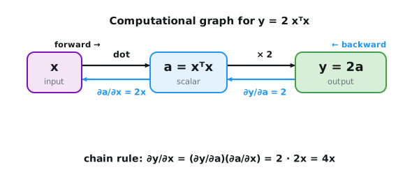
The forward pass evaluates the graph from \(\mathbf{x}\) to \(y\); to obtain the gradient, automatic differentiation then traverses it in reverse, multiplying the local derivatives along the way. We unpack computational graphs and backpropagation in full in Section 4.3, and the underlying mathematics (both modes of automatic differentiation and their costs) is developed in Section 25.3; for now we use the resulting gradients.
We can now take the gradient of y with respect to x by calling its backward method. Next, we can access the gradient via x’s grad attribute.
We can now calculate the gradient of y with respect to x by calling the gradient method.
We can now take the gradient of y with respect to x by passing through the grad transform.
We can now take the gradient of y with respect to x by calling its backward method. Next, we can access the gradient via x’s grad attribute.
y.backward()
x.grad
tensor([ 0., 4., 8., 12.])x_grad = t.gradient(y, x)
x_grad<tf.Tensor: shape=(4,), dtype=float32, numpy=array([ 0., 4., 8., 12.], dtype=float32)>from jax import grad
# The `grad` transform returns a Python function that
# computes the gradient of the original function
x_grad = grad(y)(x)
x_gradArray([ 0., 4., 8., 12.], dtype=float32)y.backward()
x.gradarray([ 0., 4., 8., 12.])We already know that the gradient of the function \(y = 2\mathbf{x}^{\top}\mathbf{x}\) with respect to \(\mathbf{x}\) should be \(4\mathbf{x}\). We can now verify that the automatic gradient computation and the expected result are identical.
x.grad == 4 * xtensor([True, True, True, True])x_grad == 4 * x<tf.Tensor: shape=(4,), dtype=bool, numpy=array([ True, True, True, True])>x_grad == 4 * xArray([ True, True, True, True], dtype=bool)x.grad == 4 * xarray([ True, True, True, True])For the new objective \(y=\sum_i x_i\), PyTorch adds the new derivative to the existing gradient buffer unless it is cleared first. This behavior supports optimizing the sum of multiple objective functions. To reset the gradient buffer, we can call x.grad.zero_() as follows:
For the new objective \(y=\sum_i x_i\), GradientTape.gradient returns a new gradient value rather than accumulating into a tensor-owned buffer.
For the new objective \(y=\sum_i x_i\), MXNet replaces the recorded gradient with the new value.
x.grad.zero_() # Reset the gradient
y = x.sum()
y.backward()
x.gradtensor([1., 1., 1., 1.])with tf.GradientTape() as t:
y = tf.reduce_sum(x)
t.gradient(y, x) # Overwritten by the newly calculated gradient<tf.Tensor: shape=(4,), dtype=float32, numpy=array([1., 1., 1., 1.], dtype=float32)>y = lambda x: x.sum()
grad(y)(x)Array([1., 1., 1., 1.], dtype=float32)with autograd.record():
y = x.sum()
y.backward()
x.grad # Overwritten by the newly calculated gradientarray([1., 1., 1., 1.])1.5.1.2 Backward for Non-Scalar Variables
When y is a vector, the most natural representation of the derivative of y with respect to a vector x is a matrix called the Jacobian that contains the partial derivatives of each component of y with respect to each component of x. Likewise, for higher-order y and x, the result of differentiation could be an even higher-order tensor.
While Jacobians do show up in some advanced machine learning techniques, more commonly we sum the gradients of each component of y with respect to the full vector x, yielding a vector of the same shape as x. For example, we often have a vector representing the value of our loss function calculated separately for each example among a batch of training examples. Here, we sum the gradients computed individually for each example.
Because deep learning frameworks vary in how they interpret gradients of non-scalar tensors, PyTorch takes some steps to avoid confusion. Invoking backward on a non-scalar elicits an error unless we tell PyTorch how to reduce the object to a scalar. More formally, we need to provide some vector \(\mathbf{v}\) such that backward will compute \(\mathbf{v}^\top \partial_{\mathbf{x}} \mathbf{y}\) rather than \(\partial_{\mathbf{x}} \mathbf{y}\). This argument is named gradient because the vector \(\mathbf{v}\) is the gradient arriving from the rest of a larger computation, as will become clear when we study backpropagation in Section 4.3. For a more detailed description, see the PyTorch documentation on the gradient argument to Tensor.backward.
By default, TensorFlow returns the gradient of the sum. In other words, rather than returning the Jacobian \(\partial_{\mathbf{x}} \mathbf{y}\), it returns the gradient of the sum \(\partial_{\mathbf{x}} \sum_i y_i\).
MXNet handles this problem by reducing all tensors to scalars by summing before computing a gradient. In other words, rather than returning the Jacobian \(\partial_{\mathbf{x}} \mathbf{y}\), it returns the gradient of the sum \(\partial_{\mathbf{x}} \sum_i y_i\).
x.grad.zero_()
y = x * x
y.backward(gradient=torch.ones(len(y)))  # Equivalently: y.sum().backward()
x.grad
tensor([0., 2., 4., 6.])with tf.GradientTape() as t:
y = x * x
t.gradient(y, x) # Same as y = tf.reduce_sum(x * x)<tf.Tensor: shape=(4,), dtype=float32, numpy=array([0., 2., 4., 6.], dtype=float32)>y = lambda x: x * x
# grad is only defined for scalar output functions
grad(lambda x: y(x).sum())(x)Array([0., 2., 4., 6.], dtype=float32)with autograd.record():
y = x * x
y.backward()
x.grad # Equals the gradient of y = sum(x * x)array([0., 2., 4., 6.])1.5.2 Controlling the Graph
Sometimes the graph the framework records is not the graph we want to differentiate. The next two subsections show how to prune it by detaching individual intermediate results, and how to switch recording off altogether.
1.5.2.1 Detaching Computation
Sometimes, we wish to move some calculations outside of the recorded computational graph. For example, say that we use the input to create some auxiliary intermediate terms for which we do not want to compute a gradient. In this case, we need to detach the respective computational graph from the final result. For example, suppose that z = x * y and y = x * x but we want to focus on the direct influence of x on z rather than the influence conveyed via y. In this case, we can create a new variable u that takes the same value as y but whose computational history is not connected to the new graph. Thus u has no ancestors in the graph and gradients do not flow through u to x. Now consider z = x * u. Because u is treated as a constant equal to \(x^2\), the gradient is \(\partial z / \partial x = u = x^2\). Had we not detached, so that z = x * (x * x) \(= x^3\), we would instead have obtained \(\partial z / \partial x = 3x^2\).
x.grad.zero_()
y = x * x
u = y.detach()
z = u * x

z.sum().backward()
x.grad == u
tensor([True, True, True, True])# Set persistent=True to preserve the compute graph.
# This lets us run t.gradient more than once
with tf.GradientTape(persistent=True) as t:
y = x * x
u = tf.stop_gradient(y)
z = u * x
x_grad = t.gradient(z, x)
x_grad == u<tf.Tensor: shape=(4,), dtype=bool, numpy=array([ True, True, True, True])>import jax
y = lambda x: x * x
# jax.lax primitives are Python wrappers around XLA operations
u = jax.lax.stop_gradient(y(x))
z = lambda x: u * x
grad(lambda x: z(x).sum())(x) == uArray([ True, True, True, True], dtype=bool)with autograd.record():
y = x * x
u = y.detach()
z = u * x
z.backward()
x.grad == uarray([ True, True, True, True])Although this procedure detaches y’s ancestors from the graph leading to z, the computational graph leading to y persists and thus we can calculate the gradient of y with respect to x.
x.grad.zero_()
y.sum().backward()
x.grad == 2 * x
tensor([True, True, True, True])t.gradient(y, x) == 2 * x<tf.Tensor: shape=(4,), dtype=bool, numpy=array([ True, True, True, True])>grad(lambda x: y(x).sum())(x) == 2 * xArray([ True, True, True, True], dtype=bool)y.backward()
x.grad == 2 * xarray([ True, True, True, True])1.5.2.2 Turning Off Gradient Tracking
Recording operations for a backward pass costs time and memory. When we only need a value (at prediction time, or while updating parameters by hand), we can skip the bookkeeping entirely.
Wrap the computation in a torch.no_grad() block (or decorate a function with @torch.no_grad()). The result still shares data with x, but it is not attached to the graph, so no gradient can flow through it.
TensorFlow only records operations executed inside a tf.GradientTape (a tape is the recorded list of executed operations), so any computation outside a tape is already untracked. To pause recording within a tape, use tape.stop_recording().
JAX never records gradients implicitly: differentiation occurs only after a transform such as grad is applied. Thus, users opt in to differentiation.
MXNet only builds a graph inside an autograd.record() block, so ordinary computation already carries no gradient bookkeeping. To suspend tracking within a recording scope, wrap the code in autograd.pause().
with torch.no_grad():
    y = 2 * torch.dot(x, x)
y.requires_grad # False: y is detached from the graphFalse# Outside any GradientTape, nothing is recorded
y = 2 * tf.tensordot(x, x, axes=1)
y<tf.Tensor: shape=(), dtype=float32, numpy=28.0># No graph is built unless we ask for it via a transform like `grad`
y = 2 * jnp.dot(x, x)
yArray(28., dtype=float32)with autograd.record():
with autograd.pause():
y = 2 * np.dot(x, x) # not recorded: no gradient will flow through y
yarray(28.)This untracked mode is the default for inference and evaluation throughout the rest of the book.
1.5.3 Beyond the Basics
Automatic differentiation extends beyond the fixed formulas considered so far: it handles arbitrary control flow, derivatives of derivatives, and even lets us choose the direction in which the graph is traversed.
1.5.3.1 Gradients and Python Control Flow
The preceding examples used a fixed sequence of operations such as z = x * x * x. Programs can instead use auxiliary variables and choose branches from intermediate results. One benefit of using automatic differentiation is that even if building the computational graph of a function required Python control flow (e.g., conditionals, loops, and arbitrary function calls), we can still calculate the gradient of the resulting variable. To illustrate this, consider the following code snippet where the number of iterations of the while loop and the evaluation of the if statement both depend on the value of the input a.
def f(a):
    b = a * 2
    while b.norm() < 1000:
        b = b * 2
    if b.sum() > 0:
        c = b
    else:
        c = 100 * b
    return c
def f(a):
b = a * 2
while tf.norm(b) < 1000:
b = b * 2
if tf.reduce_sum(b) > 0:
c = b
else:
c = 100 * b
return cdef f(a):
b = a * 2
while jnp.linalg.norm(b) < 1000:
b = b * 2
if b.sum() > 0:
c = b
else:
c = 100 * b
return cdef f(a):
b = a * 2
while np.linalg.norm(b) < 1000:
b = b * 2
if b.sum() > 0:
c = b
else:
c = 100 * b
return cBelow, we call this function, passing in a random value, as input. Since the input is a random variable, we do not know what form the computational graph will take. However, whenever we execute f(a) on a specific input, we realize a specific computational graph and can subsequently run backward.
a = torch.randn(size=(), requires_grad=True)
d = f(a)
d.backward()
a = tf.Variable(tf.random.normal(shape=()))
with tf.GradientTape() as t:
d = f(a)
d_grad = t.gradient(d, a)
d_grad<tf.Tensor: shape=(), dtype=float32, numpy=4096.0>from jax import random
a = random.normal(random.key(1), ())
d = f(a)
d_grad = grad(f)(a)a = np.random.normal()
a.attach_grad()
with autograd.record():
d = f(a)
d.backward()Even though our function f is, for demonstration purposes, a bit contrived, its dependence on the input is quite simple: it is a linear function of the scalar a with piecewise defined scale. As such, f(a) / a is a constant and, moreover, it needs to match the gradient of f(a) with respect to a.
a.grad == d / atensor(True)d_grad == d / a<tf.Tensor: shape=(), dtype=bool, numpy=True>d_grad == d / aArray(True, dtype=bool)a.grad == d / aarray(True)Dynamic control flow occurs frequently in deep learning. For instance, when processing text, the computational graph depends on the length of the input. Automatic differentiation records or traces the operations for the realized computation rather than requiring a separate derivative for every possible execution path.
1.5.3.2 Higher-Order Derivatives
Occasionally we need the derivative of a derivative: the curvature of a function, or the Hessian–vector products (products of the matrix of second derivatives, the Hessian, with a vector) used by some optimizers. Autograd can differentiate through a gradient computation. Take \(f(x) = x^3\), for which \(f'(x) = 3x^2\) and \(f''(x) = 6x\).
Pass create_graph=True so the first gradient is itself a differentiable function of x, then differentiate again.
Nest two GradientTapes: the outer tape differentiates the gradient computed under the inner tape.
grad returns a function, so we apply it twice.
Higher-order gradients in MXNet require explicitly retaining the graph of the first derivative. The mathematics is framework-agnostic and developed in Section 25.3.
x3 = torch.tensor(2.0, requires_grad=True)
dy = torch.autograd.grad(x3 ** 3, x3, create_graph=True)[0]  # 3x^2 = 12
d2y = torch.autograd.grad(dy, x3)[0]                          # 6x  = 12
dy, d2y
(tensor(12., grad_fn=<MulBackward0>), tensor(12.))x3 = tf.Variable(2.0)
with tf.GradientTape() as outer:
with tf.GradientTape() as inner:
y = x3 ** 3
dy = inner.gradient(y, x3) # 3x^2 = 12
d2y = outer.gradient(dy, x3) # 6x = 12
dy, d2y(<tf.Tensor: shape=(), dtype=float32, numpy=12.0>,
<tf.Tensor: shape=(), dtype=float32, numpy=12.0>)f = lambda x: x ** 3
dy = grad(f)(2.0) # 3x^2 = 12
d2y = grad(grad(f))(2.0) # 6x = 12
dy, d2y(Array(12., dtype=float32, weak_type=True),
Array(12., dtype=float32, weak_type=True))1.5.3.3 Forward versus Reverse Mode
Automatic differentiation can traverse the computational graph in either direction. Reverse mode, the variant we have used so far and the engine behind backpropagation, sweeps from the output back to the inputs, yielding the gradient of a single scalar with respect to all inputs in one pass. Forward mode sweeps the other way, propagating derivatives from one input outward to every output.
The choice is about cost, and a counting argument settles it. For a function with \(n\) inputs and \(m\) outputs, filling the full matrix of derivatives takes one reverse sweep per output (\(m\) sweeps) or one forward sweep per input (\(n\) sweeps), each sweep costing about as much as one evaluation of the function. A training loss is a single scalar (\(m = 1\)) depending on millions of parameters (\(n\) huge), so reverse mode delivers the entire gradient for the price of roughly one extra forward pass. Forward mode wins in the opposite regime (few inputs, many outputs), is useful for per-input sensitivities, and can participate in efficient Hessian–vector-product constructions, as in the Julia package ForwardDiff.jl (Revels et al. 2016). The exercises explore this trade-off further, and Section 25.3 derives both modes and their costs in full.
1.5.4 Discussion
Automatic differentiation frees practitioners from deriving gradients by hand, and it makes it practical to train models for which pen and paper gradient computations would be prohibitively time consuming. While we use autograd to optimize models (in a statistical sense), the optimization of autograd libraries themselves (in a computational sense) is a rich subject that matters to framework designers. Here, tools from compilers and graph manipulation are used to compute results quickly and with modest memory.
The basic workflow is: (i) attach gradients to those variables with respect to which we desire derivatives; (ii) record the computation of the target value; (iii) execute the backpropagation function; and (iv) access the resulting gradient.
1.5.5 Exercises
- Cost of second derivatives. ● The counting argument in Section 1.5.3.3 prices the gradient of a scalar loss with \(n\) parameters at roughly one extra forward pass. Use the same argument to estimate, in units of function evaluations, the cost of the full Hessian (the \(n \times n\) matrix of second derivatives) and the cost of a single Hessian–vector product. Explain the difference between the two costs.
- [code] Repeated backward passes. For an
xwithrequires_grad=True, computey = 2 * torch.dot(x, x), cally.backward(), and then cally.backward()a second time. What happens? Resetx.grad, recomputey, and repeat both calls, this time passingretain_graph=Trueto the first one. Explain what the backward pass discards by default and why, and what the second call leaves inx.grad.
- [code] Repeated backward passes. Record
y = 2 * tf.tensordot(x, x, axes=1)underwith tf.GradientTape() as t:, callt.gradient(y, x), and then call it a second time. What happens? A tape constructed withpersistent=Truekeeps its recorded operations so thatt.gradientcan be called repeatedly. Explain what this costs in memory during training, and when the memory held by a persistent tape is released.
- [code] Repeated backward passes. Call the function returned by
jax.gradtwice on the same input. Why does the second call behave no differently from the first? What does this tell you about where JAX keeps the information needed for differentiation?
- [code] Repeated backward passes. For an
xwith an attached gradient, computey = 2 * np.dot(x, x)insideautograd.record(), cally.backward(), and then cally.backward()a second time. What happens? Recordyagain and repeat both calls, this time passingretain_graph=Trueto the first one. Explain what the backward pass discards by default and why, and what the second call leaves inx.grad.
- [code] From scalar to vector input. Replace the scalar input
aof the functionfdefined in Section 1.5.3.1 by a random vector of length 5, and differentiate the sum of the entries ofd = f(a)with respect toa.- Express
f(a)in terms ofa, and give the Jacobian offataand the gradient of the sum of the entries ofd. - Compute this gradient with automatic differentiation and check whether it still equals
d / aelementwise. - Identify the inputs
aat whichfjumps, and state what automatic differentiation returns at an input next to such a point.
- Express
- [code] Manual tracing. Let \(f(x, y, z) = (x + y) \cdot z\) with \(x = -2\), \(y = 5\), and \(z = -4\).
- Draw the computational graph of \(f\) with one node per operation, compute the forward pass by hand, and trace \(\partial f/\partial x\), \(\partial f/\partial y\), and \(\partial f/\partial z\) backward from \(f\) through the multiplication and addition nodes (reverse mode).
- Compute the same three derivatives in forward mode, propagating the derivative with respect to one input at a time from the inputs to \(f\). Compare the number of sweeps each mode needs and the intermediate values each must keep in memory.
- Verify every value using automatic differentiation.
- [code] Detached intermediates. Let
y = x * xandu = y.detach(), and considerz = u * u,z = y * u, andz = y * y. For eachz, recomputeyandu, resetx.grad, and callbackwardon the sum of the components ofz. Before running any code, predict the outcome of each call, including the resultingx.grad. Check your predictions, and explain the ratio between the gradients forz = y * uandz = y * y. - [code] Manual parameter updates. Let
wbe a tensor withrequires_grad=True, computeloss = (w * w).sum(), and callloss.backward(). Perform the updatew = w - 0.1 * w.gradand inspectw.requires_grad,w.grad_fn,w.is_leaf, andw.grad. Explain what the update has done to the graph, predict what a second forward and backward pass leaves inw.grad, and check. Then perform the update in place inside atorch.no_grad()block and compare.
- [code] Detached intermediates. Let
y = x * xandu = tf.stop_gradient(y)inside a persistenttf.GradientTapet. Before running any code, predictt.gradient(z, x)for each ofz = u * u,z = y * u, andz = y * y, all computed insidet. Check your predictions, and explain the ratio between the results forz = y * uandz = y * y. - [code] Manual parameter updates. Let
wbe atf.Variable, computeloss = tf.reduce_sum(w * w)under atf.GradientTapet, and obtaing = t.gradient(loss, w).- Perform the update
w = w - 0.1 * gand inspecttype(w). Predict whatgradientreturns for a second forward pass under a new tape, check, and explain the result. - Start again from a
tf.Variable, perform the update withw.assign_sub(0.1 * g), and repeat the second forward pass. Explain why a training loop updates variables this way.
- Perform the update
- [code] Detached intermediates. Let
y = lambda x: x * xandu = jax.lax.stop_gradient(y(x)). Before running any code, predictgrad(lambda x: z(x).sum())(x)for each ofz = lambda x: u * u,z = lambda x: y(x) * u, andz = lambda x: y(x) * y(x). Check your predictions, and explain the ratio between the results forz = lambda x: y(x) * uandz = lambda x: y(x) * y(x). - [code] Manual parameter updates. Let
w = jnp.arange(4.0)andg = lambda x: (w * x).sum(), which readswfrom the enclosing scope. Predictgrad(g)(x), check, and state with respect to which arraygraddifferentiates. Then rewritegso thatgradreturns the gradient of(w * x).sum()with respect tow, use it for one update ofwwith learning rate 0.1, and explain what this implies for how a JAX training loop must pass the parameters to the loss function.
- [code] Detached intermediates. Let
y = x * xandu = y.detach(), and considerz = u * u,z = y * u, andz = y * y. For eachz, computey,u, andzafresh inside anautograd.record()scope and callz.backward(). Before running any code, predict the outcome of each call, including the resultingx.grad. Check your predictions, and explain the ratio between the gradients forz = y * uandz = y * y. - [code] Manual parameter updates. Let
wbe an array with an attached gradient, computeloss = (w * w).sum()insideautograd.record(), and callloss.backward(). Perform the updatew = w - 0.1 * w.gradoutside the recording scope and inspectw.grad. Explain what the rebinding has done to the buffer attached byattach_grad, and predict what a second recorded forward pass followed bybackwarddoes. Then perform the update asw[:] = w - 0.1 * w.gradinstead and compare.