%matplotlib inline
from d2l import torch as d2l
import copy
import math
import torch
from torch import nn9.12 Practice
The preceding sections isolated individual optimization choices. A complete training run must combine them and remain stable over a long computation. This section summarizes configurations reported for recent large-scale runs, implements gradient clipping and weight averaging, and describes a protocol for tuning and comparing optimizers.
%matplotlib inline
from d2l import jax as d2l
from flax import nnx
import jax
from jax import numpy as jnp
import math
import optax
9.12.1 Configurations Reported for Large-Scale Training
A target-scale language-model run is too expensive for an exhaustive hyperparameter sweep, so its hyperparameters are assembled from smaller proxies (Section 9.11), from precedent, and from the recipes of earlier runs. Some of what the teams settled on is public. Table 9.12.1 collects the optimizer configurations disclosed by four prominent pretraining reports from 2024–2026. The table documents these cases rather than defining a general recipe: each entry is what a team reported shipping, usually with no ablation attached, and a dash means the report does not say.
:What four pretraining reports disclose about their optimizer configuration. A dash means the report does not say. Batch sizes are quoted the way each report quotes them (tokens or sequences).
| run | optimizer | \(\beta_1, \beta_2\) | peak LR and schedule | warmup | clip | weight decay | batch size |
|---|---|---|---|---|---|---|---|
| Llama 3 405B (Grattafiori et al. 2024) | AdamW | — | \(8{\times}10^{-5}\), cosine to \(8{\times}10^{-7}\) | 8k steps | — | — | ramp 4M \(\to\) 8M \(\to\) 16M tokens |
| DeepSeek-V3 (DeepSeek-AI et al. 2024) | AdamW | 0.9, 0.95 | \(2.2{\times}10^{-4}\), constant to 10T tokens, cosine to \(2.2{\times}10^{-5}\) | 2k steps | 1.0 | 0.1 | ramp 3,072 \(\to\) 15,360 seqs over 469B tokens |
| OLMo 2 7B (Team OLMo et al. 2025) | AdamW | 0.9, 0.95 | \(3{\times}10^{-4}\), cosine to 10% of peak | 2k steps | 1.0 | 0.1, embeddings exempt | 1,024 seqs, fixed |
| Kimi K2 (Kimi Team 2025) | MuonClip | — | \(2{\times}10^{-4}\), constant to 10T tokens, cosine to \(2{\times}10^{-5}\) | 500 steps | — | 0.1 | 67M tokens, fixed |
These four reports are case studies, not a representative survey. Three report AdamW and one reports a Muon/AdamW split. Two disclose \((\beta_1,\beta_2)=(0.9,0.95)\), weight decay 0.1, and global-norm clipping at 1; the dashes in the other rows indicate missing evidence rather than implied defaults. All four report warmup followed by either cosine decay or a stable phase and later decay. Batch ramping appears in two rows and fixed batches in the other two. The table therefore shows several repeated choices and one production use of Muon, while also showing that the published fields are insufficient to reproduce any run in full.
9.12.2 Gradient Clipping
The next section examines the clipping column. Gradient clipping entered this book in Section 8.5 as the fix for exploding RNN gradients; the reports show that the method is also used beyond recurrent architectures. Every run above that discloses a threshold clips, and every disclosed threshold is 1. Global-norm clipping treats all parameters as one long vector: with \(\mathbf{g}\) the concatenation of every parameter’s gradient and \(\theta\) the threshold,
\[ \mathbf{g} \leftarrow \min\left(1,\; \frac{\theta}{\|\mathbf{g}\|_2}\right) \mathbf{g}. \tag{9.12.1}\]
A gradient shorter than \(\theta\) passes untouched; a longer one keeps its direction and loses its length. The implementation is a few lines in either framework.
clip_grad_norm_ rescales the gradients in place, between backward and step, and returns the norm it measured before clipping. We wrap an existing optimizer so the harness of Section 9.6 can use it unchanged, and we keep the returned norms, which the demonstration below will want.
In Optax, clipping is a gradient transformation like any other, so it composes with optax.chain: the clipped transformation drops into nnx.Optimizer, and the harness of Section 9.6 needs no change at all.
class Clipped:
    """Clip the global gradient norm before every optimizer step."""
    def __init__(self, optimizer, params, max_norm=1.0):
        self.optimizer = optimizer
        self.params = list(params)
        self.max_norm = max_norm
        self.norms = []

    def step(self):
        norm = nn.utils.clip_grad_norm_(self.params, self.max_norm)
        self.norms.append(float(norm))
        self.optimizer.step()

    def zero_grad(self):
        self.optimizer.zero_grad()
def clipped(tx, max_norm=1.0):
"""Clip the global gradient norm before an optimizer's update."""
return optax.chain(optax.clip_by_global_norm(max_norm), tx)9.12.2.1 Preventing a Numerical Failure
Section 9.6 swept SGD with momentum on TinyLM and found a knife’s edge: the best learning rate sat one grid point below one that returned NaN. This divergent grid point provides a direct test of whether clipping can prevent the observed numerical failure. We rerun it with and without clipping, changing nothing else.
data = d2l.TimeMachine(batch_size=64, num_steps=64, tokenization='char',
                       num_train=100000)

def final_loss(losses, k=100):
    v = sum(losses[-k:]) / k
return v if math.isfinite(v) else float('inf')curves = {}
for clip in (False, True):
torch.manual_seed(0)
model = d2l.TinyLM(len(data.vocab))
optimizer = torch.optim.SGD(model.parameters(), lr=1.0, momentum=0.9)
if clip:
optimizer = Clipped(optimizer, model.parameters())
label = 'clipped at 1.0' if clip else 'unclipped'
curves[label] = d2l.train_lm(model, data, optimizer, num_steps=2000)
print(f'{label}: final loss {final_loss(curves[label]):.3f}')
fired = sum(n > optimizer.max_norm for n in optimizer.norms)
print(f'clipping changed the update on {fired} of {len(optimizer.norms)} '
f'steps; median gradient norm '
f'{sorted(optimizer.norms)[len(optimizer.norms) // 2]:.2f}')unclipped: final loss inf
clipped at 1.0: final loss 1.052
clipping changed the update on 6 of 2000 steps; median gradient norm 0.31curves = {}
for clip in (False, True):
model = d2l.TinyLM(len(data.vocab), rngs=nnx.Rngs(0))
tx = optax.sgd(0.3, momentum=0.9)
if clip:
tx = clipped(tx)
optimizer = nnx.Optimizer(model, tx, wrt=nnx.Param)
label = 'clipped at 1.0' if clip else 'unclipped'
curves[label] = d2l.train_lm(model, data, optimizer, num_steps=2000)
print(f'{label}: final loss {final_loss(curves[label]):.3f}')unclipped: final loss inf
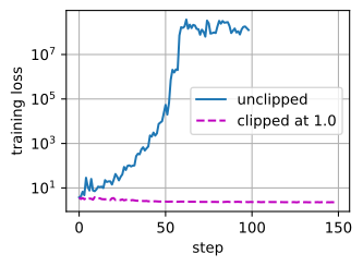
clipped at 1.0: final loss 1.067The instability occurs early, so we plot the first 150 steps on a log scale.
d2l.plot(list(range(150)), [curves[k][:150] for k in curves], 'step',
         'training loss', legend=list(curves), yscale='log')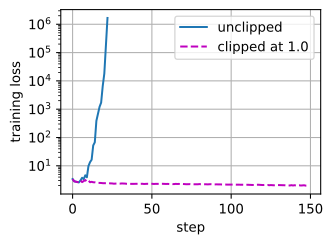
The unclipped run makes normal progress for a few steps, then feeds back on itself: an oversized step lands the iterate somewhere steeper, the gradient there is larger, momentum compounds it, and within two dozen steps the loss has climbed six orders of magnitude and overflows. The clipped run, at the identical learning rate, trains to a final loss at or slightly below the tuned unclipped run of Section 9.6. The median gradient norm was far below the threshold, and clipping changed the update on six steps out of two thousand. In these paired runs, those six interventions separate the divergent trajectory from the stable one.
The unclipped run makes progress for a moment, then feeds back on itself: an oversized step lands the iterate somewhere steeper, the gradient there is larger, momentum compounds it, and the loss climbs through four orders of magnitude before overflowing within the first couple hundred steps. The clipped run, at the identical learning rate, trains to a final loss in the range of the tuned runs of Section 9.6. The Optax combinator does not report how often it fired; the instrumented PyTorch tab counts six interventions in two thousand steps, and the picture here is the same.
This count illustrates clipping used as a guard: most updates remain unchanged, while a small number of unusually large gradients are rescaled. The tail is not an accident of our small model: gradient noise in language models is measurably heavy-tailed, and under such noise clipped SGD provably converges where plain SGD can fail (Zhang et al. 2020). The threshold can be set above the typical norms observed in a stable run. If clipping activates on most steps, it continuously normalizes or rescales the update rather than serving only as an outlier guard; the learning rate and threshold should then be tuned together (Godbole et al. 2023). For the Adam family the arithmetic differs but the conclusion holds. For a persistent gradient, Adam’s normalized update in a coordinate is on the order of \(\eta\) (Section 9.6), transiently up to a few times that: \(|\hat{m}/\sqrt{\hat{v}}|\) can briefly reach \((1 - \beta_1)/\sqrt{1 - \beta_2} \approx 3\) at the defaults. So clipping is no substitute for lowering a too-large Adam learning rate, and in our runs it was not. What it still provides is protection for the estimates: one enormous gradient otherwise enters both moment estimates, and its contribution to the slower second-moment average decays over a timescale on the order of \(1/(1-\beta_2)\) steps.
9.12.2.2 Additional Stability Methods
At trillion-token scale, clipping is one of several stability methods, most of them aimed at the places where transformer blow-ups concentrate: the attention logits and the output softmax. PaLM’s training added a z-loss, a small penalty on \(\log^2 Z\) of the softmax normalizer, to keep the output logits from drifting large (Chowdhery et al. 2022). QK-norm normalizes queries and keys immediately before their dot product, so attention logits cannot grow with the norms of what feeds them (Henry et al. 2020); OLMo 2 adopted it as part of the stability overhaul that its report documents (Team OLMo et al. 2025). MuonClip’s QK-clip rescales the query and key projections whenever the largest attention logit crosses a cap; the Kimi K2 report includes this method in a 15.5-trillion-token run with no reported loss spike (Section 9.9, (Kimi Team 2025)). And when prevention fails, the practice is unglamorous. Facing about twenty spikes in a run, the PaLM team rewound to a checkpoint a few hundred steps earlier and skipped the offending batches, after establishing that the same batches caused no spike when replayed from a different state: spikes came from state and data together, not from bad data alone (Chowdhery et al. 2022). The OPT team published its training logbook along with the model; it records two months of restarts, mid-flight learning-rate cuts, and hardware failures in a way no polished paper does, and it provides an unusually detailed public record of operational interventions during a large run (Zhang et al. 2022).
9.12.3 Weight Averaging
The chapter’s third recurring decision is living with noise, and it has one more tool, one that is nearly free. A constant-rate iterate rattles around its noise ball (Section 9.3), and a schedule quenches the rattling by decaying the rate (Section 9.8). Averaging can reduce this variability without changing the learning rate: when iterate fluctuations are weakly correlated around a region, some of them cancel in the mean. Stochastic weight averaging made this a standard trick, averaging checkpoints from the tail of training and evaluating the average (Izmailov et al. 2018). You have met the running form twice: Section 7.6 put an exponential moving average of the weights into the standard recipe, and Section 5.2 showed the state needed to maintain one. It is \(\bar{\mathbf{x}}_t = \alpha\, \bar{\mathbf{x}}_{t-1} + (1 - \alpha)\, \mathbf{x}_t\): the same leaky average this chapter has applied to gradients (momentum) and to squared gradients (Adam), now applied to the weights themselves, purely for evaluation. The training run never sees it. What is new here is the noise-ball reading of why it helps.
We test it on the schedule testbed of Section 9.8, reproduced verbatim, for its constant-learning-rate baseline, whose test accuracy plateaued and varied across epochs. Alongside the live weights we maintain an EMA with \(\alpha = 0.999\), an averaging window of about a thousand steps, roughly four epochs here.
def net_fn():
    model = nn.Sequential(
        nn.Conv2d(1, 6, kernel_size=5, padding=2), nn.BatchNorm2d(6),
        nn.ReLU(),
        nn.MaxPool2d(kernel_size=2, stride=2),
        nn.Conv2d(6, 16, kernel_size=5), nn.BatchNorm2d(16), nn.ReLU(),
        nn.MaxPool2d(kernel_size=2, stride=2),
        nn.Flatten(),
        nn.Linear(16 * 5 * 5, 120), nn.BatchNorm1d(120), nn.ReLU(),
        nn.Linear(120, 84), nn.BatchNorm1d(84), nn.ReLU(),
        nn.Linear(84, 10))
    def init_weights(m):
        if type(m) in (nn.Linear, nn.Conv2d):
            nn.init.xavier_uniform_(m.weight)
    model.apply(init_weights)
    return model

device = d2l.try_gpu()
train_iter, test_iter = d2l.load_data_fashion_mnist(batch_size=256)
loss = nn.CrossEntropyLoss()
xavier = nnx.initializers.xavier_uniform()
class Net(nnx.Module):
def __init__(self, rngs=None):
rngs = nnx.Rngs(0) if rngs is None else rngs
self.conv1 = nnx.Conv(1, 6, kernel_size=(5, 5), padding='same',
kernel_init=xavier, rngs=rngs)
self.bn1 = nnx.BatchNorm(6, rngs=rngs)
self.conv2 = nnx.Conv(6, 16, kernel_size=(5, 5), padding='valid',
kernel_init=xavier, rngs=rngs)
self.bn2 = nnx.BatchNorm(16, rngs=rngs)
self.fc1 = nnx.Linear(16 * 5 * 5, 120, kernel_init=xavier, rngs=rngs)
self.bn3 = nnx.BatchNorm(120, rngs=rngs)
self.fc2 = nnx.Linear(120, 84, kernel_init=xavier, rngs=rngs)
self.bn4 = nnx.BatchNorm(84, rngs=rngs)
self.fc3 = nnx.Linear(84, 10, kernel_init=xavier, rngs=rngs)
def __call__(self, x):
x = nnx.max_pool(nnx.relu(self.bn1(self.conv1(x))),
window_shape=(2, 2), strides=(2, 2))
x = nnx.max_pool(nnx.relu(self.bn2(self.conv2(x))),
window_shape=(2, 2), strides=(2, 2))
x = x.reshape((x.shape[0], -1))
x = nnx.relu(self.bn3(self.fc1(x)))
x = nnx.relu(self.bn4(self.fc2(x)))
return self.fc3(x)
fashion = d2l.FashionMNIST(batch_size=256)
train_iter = fashion.get_dataloader(train=True)
test_iter = fashion.get_dataloader(train=False)The EMA update walks the two state_dicts in parallel. Floating-point entries are averaged, which includes the BatchNorm running statistics, so the averaged model stays approximately consistent — an EMA of running statistics is not the exact statistic of the EMA weights; a more accurate alternative is to recompute them for the averaged weights, as the checkpoint-averaging note below prescribes. Integer buffers are copied through.
The EMA update is one tree.map over the parameters and BatchNorm statistics of the two models. Averaging the running statistics keeps the averaged model approximately consistent — an EMA of running statistics is not the exact statistic of the EMA weights; a more accurate alternative is to recompute them for the averaged weights, as the checkpoint-averaging note below prescribes.
def ema_update(ema, model, decay=0.999):
    with torch.no_grad():
        for e, p in zip(ema.state_dict().values(),
                        model.state_dict().values()):
            if e.dtype.is_floating_point:
                e.mul_(decay).add_(p, alpha=1 - decay)
            else:
                e.copy_(p)

lr, num_epochs = 0.3, 15
torch.manual_seed(0)
net = net_fn().to(device)
ema = copy.deepcopy(net)
trainer = torch.optim.SGD(net.parameters(), lr=lr)
live_acc, avg_acc = [], []
for epoch in range(num_epochs):
    net.train()
    for X, y in train_iter:
        X, y = X.to(device), y.to(device)
        trainer.zero_grad()
        loss(net(X), y).backward()
        trainer.step()
        ema_update(ema, net)
    live_acc.append(d2l.evaluate_accuracy_gpu(net, test_iter))
    avg_acc.append(d2l.evaluate_accuracy_gpu(ema, test_iter))
print(f'final test accuracy: live {live_acc[-1]:.3f}, '
      f'EMA {avg_acc[-1]:.3f}')
final test accuracy: live 0.899, EMA 0.911lr, num_epochs = 0.3, 15
model = Net(rngs=nnx.Rngs(0))
ema = nnx.clone(model)
optimizer = nnx.Optimizer(model, optax.sgd(lr), wrt=nnx.Param)
@nnx.jit
def train_step(model, optimizer, X, y):
def loss_fn(model):
return optax.softmax_cross_entropy_with_integer_labels(
model(X), y).mean()
l, grads = nnx.value_and_grad(loss_fn)(model)
optimizer.update(model, grads)
return l
@nnx.jit
def ema_step(ema, model, decay=0.999):
kinds = (nnx.Param, nnx.BatchStat) # skip any non-float state
new = jax.tree.map(lambda e, p: decay * e + (1 - decay) * p,
nnx.state(ema, kinds), nnx.state(model, kinds))
nnx.update(ema, new)
@nnx.jit
def count_correct(model, X, y):
return (model(X).argmax(axis=1) == y).sum()
def accuracy(model, data_iter):
model.eval() # use running averages in the BatchNorm layers
correct = total = 0
for X, y in data_iter:
correct += int(count_correct(model, jnp.asarray(X), jnp.asarray(y)))
total += y.shape[0]
return correct / total
live_acc, avg_acc = [], []
for epoch in range(num_epochs):
model.train()
for X, y in train_iter:
train_step(model, optimizer, jnp.asarray(X), jnp.asarray(y))
ema_step(ema, model)
live_acc.append(accuracy(model, test_iter))
avg_acc.append(accuracy(ema, test_iter))
print(f'final test accuracy: live {live_acc[-1]:.3f}, '
f'EMA {avg_acc[-1]:.3f}')final test accuracy: live 0.889, EMA 0.911d2l.plot(list(range(1, num_epochs + 1)), [live_acc, avg_acc], 'epoch',
'test accuracy', legend=['live weights', 'EMA of weights'])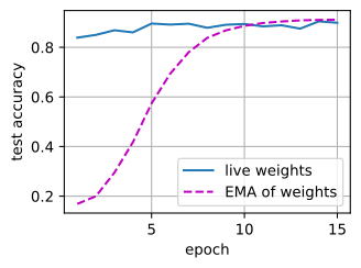
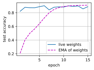
Two curves, two lessons. First, the EMA needs its window to fill before it is worth anything: for the first several epochs it trails badly, because the average still carries heavy weight on stale, near-initialization iterates. This is lag, not the zero-initialization deficit that Adam’s bias correction removes (Section 9.6): the average starts at the initial weights, so its coefficients already sum to one and there is nothing to correct — the early average retains substantial weight on old iterates. That lag is why practical EMAs either warm up the decay or start averaging late. Second, after the window fills, the EMA curve is higher and less variable than the live-weight curve in this run. It ends roughly 0.5–1 percentage point higher, while reducing sensitivity to the particular stopping epoch. The averaged model at a constant rate lands in the range the decayed schedules of Section 9.8 reached, consistent with the schedule-free discussion in that section: decay reduces the noise injected into future iterates, whereas averaging reduces variation in the evaluated parameters. That also predicts a limit. Add the same EMA to a run whose schedule already decayed well, and on a model this size the remaining nudge is too small to call from a single run. The technique is most useful when a comparable decayed endpoint is expensive to reach or no decay is planned. Its principal memory cost is one additional copy of the parameters, as discussed in Section 9.7. One footnote for checkpoint averaging: if you average a few saved checkpoints instead of keeping a running EMA, the BatchNorm statistics belong to none of the averaged weights, so recompute them with a pass over the training data before trusting the result.
9.12.3.1 Averaging at Scale
Large-scale pipelines use several forms of weight averaging. Averaging the latest \(k\) checkpoints of an LLM run, uniformly rather than exponentially, can produce a loss comparable to a later single checkpoint (Kaddour 2022), and the top row of Table 9.12.1 does it in production: the Llama 3 model that shipped is the average of checkpoints from its final annealing phase (Grattafiori et al. 2024). Model soups push the idea past a single run, averaging separately fine-tuned models into one, with accuracy gains at no inference cost (Wortsman et al. 2022). Diffusion-model training commonly evaluates an EMA of the weights (Chapter 17) and sample quality can depend strongly on the averaging window; Karras et al. (2024) developed a method to reconstruct multiple EMA windows after training so that the window can be tuned. The difference from the classifier example may partly reflect the repeated application of a denoiser during sampling, but this comparison alone does not establish the mechanism.
9.12.4 How to Tune
Every comparison in this chapter depends on a tuning protocol, which must be reported as part of the method. Google’s Tuning Playbook (Godbole et al. 2023) provides a useful vocabulary. In any experiment, split the hyperparameters into three classes: scientific hyperparameters, the ones your question is about; nuisance hyperparameters, which must be re-optimized for every setting of the scientific ones before the comparison means anything; and fixed hyperparameters, held constant and acknowledged as limits on the claim. The playbook’s rule is that a comparison is a statement about scientific hyperparameters only after the nuisances have been re-tuned per arm, and its most common instance is also the most common failure in published comparisons: the learning rate is usually a nuisance, and one shared learning rate can favor a method whose preferred scale happens to match it.
This vocabulary names what the chapter has been doing since Section 9.6. In each comparison, the optimizer was the scientific hyperparameter; the learning rate was the nuisance, re-tuned per contestant on a four-point grid spaced by factors of about three; steps, batch size, initialization, and the absence of a schedule were fixed and stated, which is why every conclusion was phrased as conditional on that protocol. At larger scale, the same design includes more nuisance dimensions (peak rate, decay horizon, warmup, and weight decay), may replace a coarse grid with quasi-random search, and separates broad exploration from a narrower final sweep. Conclusions need to be reassessed when these nuisance parameters are not retuned. Schmidt et al. (2021) benchmarked fifteen optimizers across many problems and found that trying several optimizers at default settings works about as well as extensively tuning a single one. Read it as consolation or as warning: defaults encode a lot of accumulated tuning, and an untuned comparison measures effort, not algorithms. Section 9.9’s deflation of headline speedups is the same lesson with larger budgets.
Budgets shape the rest. With a handful of runs, take the consensus column of Table 9.12.1 as given and spend every run on the peak learning rate. With tens of runs, add weight decay and the schedule, and sweep jointly only what is genuinely coupled: \(\eta\) and \(\lambda\) act through their product (Section 9.7), so a joint grid should cover both their product and deviations from a constant-product ridge. Past that, you are running a study, and the playbook is the reference. On the models of this chapter a run cost seconds to minutes, which is why we could afford the middle tier everywhere; one purpose of Section 9.11 was to keep that affordability relevant as models grow.
Finally, maintain a reproducible experiment log. For every run, record the full configuration, including the hyperparameters you consider fixed, the code version, the seed, and the one thing you changed. Vary one factor at a time when estimating a marginal effect, and use factorial designs when interactions are the question. Retain diverged runs: the NaN edge of a sweep marks the stability boundary, and Section 9.6 read its NaN column as data, not as failure. Write the conclusion next to the curves while you still believe it, because a directory of loss curves with no sentences attached goes stale within weeks. Assignments in the CS336 mold now grade the experiment log alongside the final loss, emphasizing that the experimental record is part of the result.
9.12.5 Topics Covered Elsewhere
Three method families were left out on purpose. Sharpness-aware minimization takes an inner ascent step before each descent step to seek the flat minima whose connection to generalization Section 4.5 discussed; it doubles the gradient cost, and the cited results establish improvements mainly in vision tasks rather than large-scale pretraining (Foret et al. 2021). Variance-reduction methods of the SVRG family have an elegant theory for finite sums but have not produced consistent improvements on deep networks; Section 26.2.5 presents the theory and a careful post-mortem. LARS and LAMB are layerwise-adaptive methods developed for large-batch training. In the cited benchmark, after nuisance hyperparameters were retuned, standard momentum and AdamW matched them at the studied batch sizes (Nado et al. 2021).
The remaining questions concern placement rather than optimization. This chapter analyzed optimizer state (Section 9.7) on a single device. Spreading gradients and state across a data-parallel group, ZeRO-style sharding, and the overlap of communication with computation belong to Chapter 13 and the training-systems material of Section 30.6. The updates computed there are the ones derived here; the systems side decides where the bytes live and when they move.
9.12.6 Summary
The four reports document repeated choices without defining a complete or representative recipe. Among disclosed fields, AdamW, \((0.9,0.95)\) moment coefficients, weight decay 0.1, clipping at 1, warmup, and later decay recur; one report uses a Muon/AdamW split. Clipping can guard against rare, heavy-tailed gradients, but frequent activation changes the update rule and must be tuned with the learning rate. Large runs also report z-loss, QK-norm, QK-clip, checkpoint recovery, and batch skipping. On our single-seed testbed, weight averaging raises and stabilizes endpoint accuracy; large language-model and diffusion pipelines also use checkpoint or exponential averaging. Fair optimizer comparisons identify scientific, nuisance, and fixed hyperparameters, retune nuisance parameters per arm, and retain a reproducible experiment log.
The methods in this chapter address three related decisions: how gradients are transformed into an update direction; how the step scale changes during training; and how sampling noise is managed through batching, momentum, and averaging. The configuration table gives coordinated settings of all three. When a run misbehaves, first determine which decision is responsible. Optimizers change, but this decomposition has remained useful for decades.
9.12.7 Exercises
- [code] A ten-run budget. Using AdamW on
TinyLM, reach a training loss of 1.1 in as few steps as you can, tuning only the learning rate, with a budget of ten runs. A run reaches the target at the first step at which the mean of its last 100 training losses falls below 1.1. Cap each run at 2,000 steps. Keep the log that Section 9.12.4 asks for: for every run, the learning rate, the steps taken, the final loss, and the one-sentence conclusion you drew before launching the next run. Report the log, not just the winning configuration. - [code] Batch size and the tuned rate. ● Rebuild
datawith a batch size of 256 instead of 64. At both batch sizes, train AdamW without weight decay onTinyLMfrom the same initialization at a constant learning rate, sweeping \(\eta \in \{0.5, 1, 2, 4, 8, 16, 32\} \times 10^{-3}\). Give both batch sizes the same number of training sequences: 2,000 steps at batch size 64 and 500 steps at batch size 256.- Where does the optimum move, and how does the shift compare with the square-root and linear rules of Equation 9.10.4?
- What would you have concluded about AdamW at batch size 256 had you reused the batch-64 learning rate without retuning?
- [code] Clipping regimes. The demonstration in Section 9.12.2.1 clips at \(\theta = 1\).
- Implement global-norm clipping Equation 9.12.1 yourself as a function that rescales the gradients by \(\min(1, \theta / (\|\mathbf{g}\|_2 + 10^{-6}))\) and also returns the norm before clipping. Check that at \(\theta = 1\) it reproduces the final loss of the clipped run.
- Sweep \(\theta \in \{0.01, 0.1, 0.5, 1, 4, \infty\}\) on the divergent run, recording the final loss and the fraction of steps on which clipping changed the update. Classify each threshold as a guard (fires rarely), a brake (fires on most steps), or absent, and relate each class to whether the run diverges and to its final loss.
- Show that for SGD without momentum, clipping that fires on every step turns the update into normalized gradient descent with step size \(\eta\theta\). The divergent run uses momentum \(\beta = 0.9\) in Equation 9.5.2. Bound the length of one of its updates when clipping fires on every step. Explain why neither case is the same as training at a lower learning rate.
- The decay timescale. The horizon of Section 9.7.3.3 is \(\tau = B/(\eta\lambda D)\) epochs for batch size \(B\) and dataset size \(D\), both in tokens. The DeepSeek-V3 and OLMo 2 reports in Table 9.12.1 use sequences of 4,096 tokens and training sets of about 14.8 trillion and 4 trillion tokens.
- Compute \(\tau\) for both rows at their peak learning rates. What fraction of each dataset does the averaging horizon span?
- Following Bergsma et al. (2025), what should happen to \(\lambda\) if the batch size were doubled and \(\tau\) is to be preserved, and what if instead the dataset were doubled?
- [code] The averaging window. Sweep the EMA decay \(\alpha \in \{0.9, 0.99, 0.999, 0.9999\}\) in the demonstration of Section 9.12.3 and plot the EMA’s test accuracy per epoch for each value.
- Express each averaging window \(1/(1-\alpha)\) in epochs. Derive the total weight that the EMA still places on the initial weights after the \(T \approx 3{,}500\) steps of the 15-epoch run, and evaluate it for each \(\alpha\).
- Use these numbers to explain the curves at the two ends of the sweep.
- Defaults against a small budget. Schmidt et al. (2021) found that trying several optimizers at default settings works about as well as tuning a single one. Test this on
TinyLMwith runs that Section 9.6 and Section 9.9 already made under the same protocol. As the default runs, take SGD with momentum \(0.9\) at \(\eta = 0.1\), Adam at \(\eta = 10^{-3}\), andmuon_adamwat \(\eta = 10^{-3}\), the rate that RMS matching makes comparable to Adam’s default.- Compare the best of the three default runs with the best point of each of the four grids: SGD and Adam in Section 9.6, AdamW and
muon_adamwin Section 9.9. Which optimizers, tuned alone, beat the best default run, and by how much in final loss? - Given a fixed budget of four runs on an unfamiliar problem, which strategy would you choose, and on what does the answer depend?
- Compare the best of the three default runs with the best point of each of the four grids: SGD and Adam in Section 9.6, AdamW and
- Logit drift. The z-loss of PaLM (Chowdhery et al. 2022) adds \(\kappa \log^2 Z\) to the cross-entropy, where \(Z = \sum_j \exp(o_j)\) is the softmax normalizer of the output logits \(\mathbf{o}\) and \(\kappa = 10^{-4}\).
- Show that adding the same constant \(c\) to every logit leaves the cross-entropy unchanged, and compute how the shift changes \(\log Z\) and the z-loss.
- Compute the gradient of \(\kappa \log^2 Z\) with respect to \(\mathbf{o}\). In which direction does a gradient step move the logits when \(\log Z\) is large and positive? Show that the gradient of the cross-entropy alone has no component along the all-ones vector, and explain what this implies for the overall level of the logits during training.