%matplotlib inline
from d2l import torch as d2l
import numpy as np26.6 Duality
An iterative solver stops when its progress becomes small and reports that it has converged. Whether the point it returns is optimal is a separate question. Without constraints, a zero gradient answers it for a convex function (Section 26.2). The previous section showed that a constrained optimum usually has a nonzero gradient, so that test is gone. Solvers need a lower bound on the optimal value to decide when to stop, and proofs need one to show that an answer is optimal. This section asks how to find such a bound, and what the multipliers of the previous section measure.
The clipping problem of the previous section shows the difficulty. It minimized the squared distance \(\tfrac12\|\mathbf{x} - \mathbf{x}_0\|^2\) to \(\mathbf{x}_0 = (3, 4)\) over all \(\mathbf{x}\) with \(\|\mathbf{x}\| \le 1\) and found \(\mathbf{x}^\star = (0.6, 0.8)\) with value \(8\). Suppose instead that an iterative solver stops at \(\mathbf{x} = (0.55, 0.835)\). This point is feasible (\(\|\mathbf{x}\|^2 = 0.9997\)) and has value \(8.01\). Is that good enough, or is there a feasible point with value \(7\)? The gradient at the true optimum is \((-2.4, -3.2)\), not zero, and the disk has infinitely many points, so we cannot check them all.
The bound comes from moving the constraint into the objective. Add \(\lambda\) times the constraint function \(\tfrac12(\|\mathbf{x}\|^2 - 1)\), with \(\lambda \ge 0\). At every feasible point the added term is at most zero, so the minimum of the new objective over all of \(\mathbb{R}^2\) lies below the constrained optimum. Each \(\lambda\) gives one lower bound, computed by an unconstrained minimization, and \(\lambda = 4\) gives exactly \(8\): the solver’s \(8.01\) is within \(0.01\) of optimal. Choosing the best \(\lambda\) is a second optimization problem, the dual problem. The dual problem is always convex. For a convex problem with a strictly feasible point, its value equals the constrained optimum. Its solution, the vector of multipliers, measures how fast the optimum improves when each constraint is relaxed.
We prove that no feasible point of the clipping problem beats \(\mathbf{x}^\star\), compute duals by hand for a half-plane, the support vector machine, and a power allocation problem, and show a problem whose best bound stays strictly below its optimum. All computations are small enough for NumPy, and d2l supplies the plots.
%matplotlib inline
from d2l import tensorflow as d2l
import numpy as np%matplotlib inline
from d2l import jax as d2l
import numpy as np%matplotlib inline
from d2l import mxnet as d2l
import numpy as np26.6.1 The Dual Problem
We want to prove that no feasible point of the clipping problem has a value below \(8\), without visiting feasible points. Every bound in this section comes from one fact: at a feasible point, every inequality constraint function is at most zero. We use it first on the clipping problem, with a single multiplier, and then on the general problem.
26.6.1.1 A Lower Bound from One Multiplier
The clipping problem minimizes \(f(\mathbf{x}) = \tfrac12\|\mathbf{x} - \mathbf{x}_0\|^2\) with \(\mathbf{x}_0 = (3, 4)\), subject to \(g(\mathbf{x}) = \tfrac12(\|\mathbf{x}\|^2 - 1) \le 0\). The factor \(\tfrac12\) makes the constraint’s gradient equal to \(\mathbf{x}\). The previous section found the answer \(\mathbf{x}^\star = \mathbf{x}_0 / \|\mathbf{x}_0\| = (0.6, 0.8)\) with value \(p^\star = \tfrac12(5 - 1)^2 = 8\), and the multiplier \(\lambda^\star = 4\) from the stationarity condition \(\nabla f(\mathbf{x}^\star) + \lambda^\star \mathbf{x}^\star = (-2.4, -3.2) + 4\,(0.6, 0.8) = \mathbf{0}\).
Take any \(\lambda \ge 0\) and any feasible \(\mathbf{x}\). Since \(g(\mathbf{x}) \le 0\), the product \(\lambda g(\mathbf{x})\) is at most zero, and \(f(\mathbf{x}) + \lambda g(\mathbf{x}) \le f(\mathbf{x})\). The minimum of the left side over all of \(\mathbb{R}^2\) is at most its value at this feasible \(\mathbf{x}\), and hence at most \(f(\mathbf{x})\). Taking the best feasible \(\mathbf{x}\) on the right gives
\[ \min_{\mathbf{x} \in \mathbb{R}^2} \bigl[ f(\mathbf{x}) + \lambda g(\mathbf{x}) \bigr] \;\le\; \min_{\|\mathbf{x}\| \le 1} f(\mathbf{x}) \;=\; p^\star \qquad \textrm{for every } \lambda \ge 0 . \]
The left side is a minimization without any constraint, and its value is a lower bound on the constrained optimum.
We compute it. The function being minimized is the Lagrangian \(\mathcal{L}(\mathbf{x}, \lambda) = \tfrac12\|\mathbf{x} - \mathbf{x}_0\|^2 + \tfrac\lambda2(\|\mathbf{x}\|^2 - 1)\). For \(\lambda \ge 0\) it is a convex quadratic in \(\mathbf{x}\) with Hessian \((1 + \lambda)\mathbf{I}\), so its minimizer is the point where the gradient \((\mathbf{x} - \mathbf{x}_0) + \lambda \mathbf{x}\) vanishes: \(\mathbf{x}(\lambda) = \mathbf{x}_0 / (1 + \lambda)\). The minimizer shrinks \(\mathbf{x}_0\) toward the origin, more strongly for larger \(\lambda\). To substitute it, we use \(\mathbf{x}(\lambda) - \mathbf{x}_0 = -\lambda\mathbf{x}_0 / (1 + \lambda)\) and \(\|\mathbf{x}_0\|^2 = 25\), so \(\tfrac12\|\mathbf{x}(\lambda) - \mathbf{x}_0\|^2 = \tfrac{25}{2}\lambda^2/(1+\lambda)^2\) and \(\|\mathbf{x}(\lambda)\|^2 = 25/(1+\lambda)^2\). The two terms with the factor \(25/(1+\lambda)^2\) add up to \(\tfrac{25}{2}(\lambda^2 + \lambda)/(1+\lambda)^2\), and the minimum value is
\[ q(\lambda) \;=\; \frac{25}{2}\,\frac{\lambda}{1 + \lambda} \;-\; \frac{\lambda}{2}. \tag{26.6.1}\]
The first term rises toward \(12.5\) as \(\lambda\) grows. The second term, \(\lambda\) times the constant \(-\tfrac12\) in the constraint function, falls without bound. The best bound balances the two.
A few values make this concrete. The function gives \(q(0) = 0\), \(q(1) = 5.75\), \(q(2) = 7.33\), \(q(3) = 7.875\), \(q(4) = 8\), \(q(5) = 7.92\) and \(q(8) = 7.11\). Every one of them is a valid lower bound on \(p^\star\). Its derivative \(q'(\lambda) = \tfrac{25}{2(1 + \lambda)^2} - \tfrac12\) vanishes where \((1 + \lambda)^2 = 25\), at \(\lambda = 4\), and \(q''(\lambda) = -25/(1 + \lambda)^3 < 0\), so \(\lambda = 4\) is the maximum, with value \(q(4) = 10 - 2 = 8 = p^\star\). The best bound equals the optimum, and the \(\lambda\) that attains it is the KKT multiplier. The solver’s \(8.01\) is therefore within \(0.01\) of optimal. Even \(\lambda = 3\), picked without solving anything, proves that it is within \(0.135\).
Why is \(\lambda = 4\) the right value? The constraint value at the shrunken point is \(g(\mathbf{x}(\lambda)) = \tfrac12\bigl(25/(1 + \lambda)^2 - 1\bigr)\). For \(\lambda < 4\) it is positive: the multiplier is too small to keep the minimizer in the disk (\(\mathbf{x}(1) = (1.5, 2)\) has norm \(2.5\)), and the bound is the value of an infeasible point. For \(\lambda > 4\) it is negative: the minimizer is pushed deep inside (\(\mathbf{x}(8)\) has norm \(\tfrac59\)), and the term \(\lambda g(\mathbf{x}(\lambda)) < 0\) lowers the bound. At \(\lambda = 4\) the minimizer \(\mathbf{x}(4) = (0.6, 0.8)\) lies on the circle, the added term vanishes, and the bound is the value of a feasible point.
Do these values, and the best bound of \(8\), follow from the definition \(f + \lambda g\) without the closed form for \(q\)? The cell below minimizes the Lagrangian through \(\mathbf{x}(\lambda)\), evaluates the bound on a grid of \(\lambda\), and plots it against \(p^\star\).
x0 = np.array([3.0, 4.0])                             # the point to clip
f = lambda x: 0.5 * np.sum((x - x0) ** 2)             # objective
g = lambda x: 0.5 * (np.sum(x ** 2) - 1.0)            # constraint g(x) <= 0
x_of = lambda lam: x0 / (1 + lam)                     # minimizer of L(., lam)
q = lambda lam: f(x_of(lam)) + lam * g(x_of(lam))     # dual function
p_star = f(x0 / np.linalg.norm(x0))                   # value at the clipped point
print('p* =', p_star)
print('q(0), ..., q(5) =', np.round([q(l) for l in range(6)], 4))
lams = np.linspace(0.0, 12.0, 1201)
qs = np.array([q(l) for l in lams])
print(f'max q = {qs.max():.4f} at lambda = {lams[qs.argmax()]:.2f}')
print('q <= p* everywhere:', bool((qs <= p_star + 1e-12).all()))
d2l.plot(lams, [qs, np.full_like(lams, p_star)], 'lambda', 'value',
legend=['dual function q(lambda)', 'p* = 8'])p* = 8.0
q(0), ..., q(5) = [0. 5.75 7.3333 7.875 8. 7.9167]
max q = 8.0000 at lambda = 4.00
q <= p* everywhere: True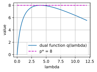
p* = 8.0
q(0), ..., q(5) = [0.     5.75   7.3333 7.875  8.     7.9167]
max q = 8.0000 at lambda = 4.00
q <= p* everywhere: True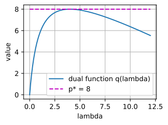
p* = 8.0
q(0), ..., q(5) = [0.     5.75   7.3333 7.875  8.     7.9167]
max q = 8.0000 at lambda = 4.00
q <= p* everywhere: True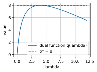
p* = 8.0
q(0), ..., q(5) = [0.     5.75   7.3333 7.875  8.     7.9167]
max q = 8.0000 at lambda = 4.00
q <= p* everywhere: True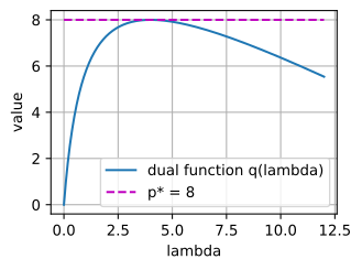
The grid maximum is \(8\), at \(\lambda = 4\), and no grid value exceeds \(p^\star\). The curve is concave and stays below the line \(p^\star = 8\), touching it once. Every value is a bound, the best bound is the optimum, and the \(\lambda\) that attains it is the KKT multiplier.
26.6.1.2 The Lagrange Dual Function
Nothing in this argument used the shape of the disk. The general problem of Section 26.5.2 minimizes \(f\) subject to inequality and equality constraints,
\[ \min_{\mathbf{x} \in \mathcal{D}}\; f(\mathbf{x}) \quad \textrm{subject to} \quad g_i(\mathbf{x}) \le 0,\; i = 1, \ldots, m, \qquad h_j(\mathbf{x}) = 0,\; j = 1, \ldots, p, \]
with optimal value \(p^\star\), the infimum of \(f\) over the feasible points (\(p^\star = +\infty\) if there are none). The set \(\mathcal{D}\) is the domain of the problem, where \(f\) and all constraint functions are defined: it is \(\mathbb{R}^n\) unless a problem keeps a set as a hard constraint, as the gap example at the end of this section does with \([0, 1]\). The Lagrangian adds one multiplier per constraint,
\[ \mathcal{L}(\mathbf{x}, \boldsymbol{\lambda}, \boldsymbol{\nu}) = f(\mathbf{x}) + \sum_{i=1}^m \lambda_i\, g_i(\mathbf{x}) + \sum_{j=1}^p \nu_j\, h_j(\mathbf{x}), \]
with \(\lambda_i \ge 0\) and \(\nu_j\) of either sign. We write \(\boldsymbol{\lambda} \succeq 0\) for “every \(\lambda_i \ge 0\)”, the elementwise sense of \(\succeq\) on vectors.
The bound of the clipping problem becomes a function of the multipliers. The Lagrange dual function is the minimum of the Lagrangian over the domain, for fixed multipliers,
\[ q(\boldsymbol{\lambda}, \boldsymbol{\nu}) = \inf_{\mathbf{x} \in \mathcal{D}}\; \mathcal{L}(\mathbf{x}, \boldsymbol{\lambda}, \boldsymbol{\nu}). \tag{26.6.2}\]
Thus \(q\) asks how low \(f\) can go once the constraints are replaced by penalties with the given weights. For the clipping problem it is Equation 26.6.1. The infimum need not be attained or even finite. Minimize \(x\) subject to \(-x \le 0\): the Lagrangian \((1 - \lambda)x\) is unbounded below unless \(\lambda = 1\), so \(q(1) = 0\) and \(q(\lambda) = -\infty\) for every other \(\lambda\). A value \(-\infty\) is a true but useless bound. The set where \(q > -\infty\) is the effective domain of \(q\); in the SVM dual below, this restriction turns into an equality constraint.
The dual function has two properties that need no assumption on \(f\), \(g_i\), or \(h_j\).
Proposition (the dual function is concave). For any primal problem, \(q(\boldsymbol{\lambda}, \boldsymbol{\nu})\) in Equation 26.6.2 is concave.
Proof. For each fixed \(\mathbf{x}\), the map \((\boldsymbol{\lambda}, \boldsymbol{\nu}) \mapsto \mathcal{L}(\mathbf{x}, \boldsymbol{\lambda}, \boldsymbol{\nu})\) is affine, because the multipliers enter linearly. The dual function is the pointwise infimum of this family of affine functions. Its hypograph, the set of points on or below its graph, is the intersection of the half-spaces below the affine functions, and an intersection of convex sets is convex. So \(q\) is concave. \(\blacksquare\)
Proposition (weak duality). If \(\mathbf{x}\) is feasible and \(\boldsymbol{\lambda} \succeq 0\), then \(q(\boldsymbol{\lambda}, \boldsymbol{\nu}) \le f(\mathbf{x})\). Consequently
\[ d^\star \;=\; \sup_{\boldsymbol{\lambda} \succeq 0,\, \boldsymbol{\nu}} q(\boldsymbol{\lambda}, \boldsymbol{\nu}) \;\le\; \inf_{\mathbf{x}\ \textrm{feasible}} f(\mathbf{x}) \;=\; p^\star. \tag{26.6.3}\]
Proof. For feasible \(\mathbf{x}\), each \(\lambda_i g_i(\mathbf{x}) \le 0\) (nonnegative times nonpositive) and each \(\nu_j h_j(\mathbf{x}) = 0\), so
\[ q(\boldsymbol{\lambda}, \boldsymbol{\nu}) \;\le\; \mathcal{L}(\mathbf{x}, \boldsymbol{\lambda}, \boldsymbol{\nu}) \;=\; f(\mathbf{x}) + \sum_i \lambda_i g_i(\mathbf{x}) + \sum_j \nu_j h_j(\mathbf{x}) \;\le\; f(\mathbf{x}). \]
Take the supremum over \((\boldsymbol{\lambda}, \boldsymbol{\nu})\) on the left and the infimum over feasible \(\mathbf{x}\) on the right. \(\blacksquare\)
This is the inequality that made every value \(q(\lambda)\) of the clipping problem a bound. The dual problem maximizes \(q\) over \(\boldsymbol{\lambda} \succeq 0\) and \(\boldsymbol{\nu}\). It is always a convex problem, a concave function maximized over a convex set, even when the primal problem is not convex. Its optimal value \(d^\star\) is a lower bound on \(p^\star\), and every dual feasible point gives one. For instance, \(q(3) = 7.875\) proves that no point of the disk has objective value below \(7.875\), without evaluating \(f\) at a single point of the disk. The difference \(p^\star - d^\star \ge 0\) is the duality gap. It was zero for the clipping problem, and the last worked example of this section shows a problem where it is not.
26.6.2 The Convex Conjugate
Computing \(q\) needs an unconstrained minimization for every value of the multipliers. For linear constraints this minimization has a structure that lets us do it once and for all. With constraints \(\mathbf{A}\mathbf{x} \preceq \mathbf{b}\) the Lagrangian is \(f(\mathbf{x}) + \boldsymbol{\lambda}^\top(\mathbf{A}\mathbf{x} - \mathbf{b})\), so
\[ q(\boldsymbol{\lambda}) = \inf_{\mathbf{x}} \bigl[ f(\mathbf{x}) + (\mathbf{A}^\top\boldsymbol{\lambda})^\top \mathbf{x} \bigr] - \mathbf{b}^\top \boldsymbol{\lambda}. \]
The infimum depends on \(f\) and on one vector, \(\mathbf{A}^\top\boldsymbol{\lambda}\), and not otherwise on \(\mathbf{A}\) or \(\mathbf{b}\). If we tabulate, once for each \(f\), the value of \(\inf_{\mathbf{x}} [f(\mathbf{x}) - \mathbf{y}^\top\mathbf{x}]\) as a function of \(\mathbf{y}\), then every linearly constrained dual with objective \(f\) can be read off the table. That table is the convex conjugate.
26.6.2.1 Supporting Lines
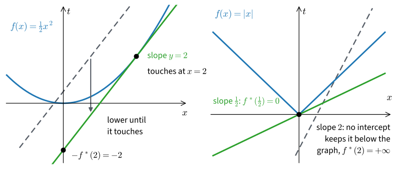
Start in one dimension with \(f(x) = \tfrac12 x^2\) and the slope \(y = 2\). Which lines \(t = 2x + c\) of slope \(2\) stay below the graph? We need \(2x + c \le \tfrac12 x^2\) for every \(x\), that is, \(c \le \min_x (\tfrac12 x^2 - 2x) = -2\), attained at \(x = 2\). The highest such line, \(t = 2x - 2\), touches the parabola at \((2, 2)\), where its slope matches \(f'(2) = 2\). Lowering a line of slope \(2\) until it touches the graph thus puts its intercept at \(-2\), and the number \(\max_x (2x - \tfrac12 x^2) = 2\) is minus that intercept. Figure 26.6.1(a) draws this.
The convex conjugate (or Fenchel–Legendre transform) of a function \(f : \mathbb{R}^n \to \mathbb{R} \cup \{+\infty\}\) records this number for every slope:
\[ f^*(\mathbf{y}) \;=\; \sup_{\mathbf{x}} \;\left( \mathbf{y}^\top \mathbf{x} - f(\mathbf{x}) \right). \tag{26.6.4}\]
Thus \(f^*(\mathbf{y})\) is minus the intercept of the highest affine function with slope \(\mathbf{y}\) that lies below the graph of \(f\). The conjugate describes \(f\) by its supporting lines instead of its values. For \(f(x) = \tfrac12 x^2\) and any \(y\) the supremum is attained at \(x = y\), so \(f^*(y) = \tfrac12 y^2\). For example, \(f^*(-1) = \tfrac12\).
Two conventions hold from here on. In this section a star \(\star\) marks an optimum and an asterisk \(*\) a conjugate. We also allow \(f\) to take the value \(+\infty\), which encodes a domain. Points where \(f = +\infty\) never attain the supremum, and convexity of such a function means convexity of its epigraph.
The supremum can be \(+\infty\). For \(f(x) = |x|\) and slope \(2\), \(2x - |x| = x\) for \(x > 0\), which grows without bound: no line of slope \(2\) stays below the V, whatever its intercept. For \(|y| \le 1\) instead, \(yx - |x| \le 0\) with equality at \(x = 0\), so the line of slope \(y\) through the origin is a supporting line. Hence \(f^*(y) = 0\) for \(|y| \le 1\) and \(f^*(y) = +\infty\) otherwise (Figure 26.6.1(b)). The conjugate of the absolute value is the indicator of the interval \([-1, 1]\), the function that is \(0\) on the set and \(+\infty\) off it.
Two properties follow directly from the definition. First, \(f^*\) is convex for every \(f\), convex or not. For fixed \(\mathbf{x}\) the expression \(\mathbf{y}^\top\mathbf{x} - f(\mathbf{x})\) is affine in \(\mathbf{y}\), and a pointwise supremum of affine functions is convex, because its epigraph is the intersection of the half-spaces above them. The same argument with an infimum made \(q\) concave, and the next subsection shows that the two facts are connected.
Second, the definition gives \(f^*(\mathbf{y}) \ge \mathbf{y}^\top\mathbf{x} - f(\mathbf{x})\) for every \(\mathbf{x}\), which rearranges into the Fenchel–Young inequality,
\[ \mathbf{y}^\top \mathbf{x} \;\le\; f(\mathbf{x}) + f^*(\mathbf{y}) \qquad \textrm{for all } \mathbf{x}, \mathbf{y}. \tag{26.6.5}\]
Equality holds exactly when \(\mathbf{x}\) attains the supremum in Equation 26.6.4. For a differentiable convex \(f\) this happens exactly when \(\mathbf{y} = \nabla f(\mathbf{x})\), since \(\mathbf{x} \mapsto \mathbf{y}^\top\mathbf{x} - f(\mathbf{x})\) is then concave and maximized where its gradient vanishes. Convexity is needed. The double well \(\phi_0(x) = (x^2 - 1)^2\) has \(\phi_0'(0) = 0\), but \(\phi_0^*(0) = -\min\phi_0 = 0\) and \(\phi_0(0) + \phi_0^*(0) = 1 > 0\), because \(x = 0\) is a local maximum of \(\phi_0\), not a point where the line of slope \(0\) touches from below. For the self-conjugate pair \(\tfrac12\|\mathbf{x}\|^2\), Fenchel–Young becomes the familiar \(\mathbf{y}^\top\mathbf{x} \le \tfrac12\|\mathbf{x}\|^2 + \tfrac12\|\mathbf{y}\|^2\).
Does the conjugate lose information? For a convex \(f\) that is proper (never \(-\infty\) and not \(+\infty\) everywhere) and closed (its epigraph is a closed set), the supporting lines determine the graph, and applying the conjugate twice recovers it: \(f^{**} = f\) (Rockafellar 1970). For a nonconvex \(f\) that has at least one affine function below it, \(f^{**}\) is the largest closed convex function below \(f\), its convex envelope (Exercise 1d).
The pairs used in this section and its exercises are:
- \(\tfrac12\|\mathbf{x}\|^2\) and \(\tfrac12\|\mathbf{y}\|^2\), the self-conjugate pair;
- \(\tfrac12\mathbf{x}^\top\mathbf{A}\mathbf{x}\) and \(\tfrac12\mathbf{y}^\top\mathbf{A}^{-1}\mathbf{y}\) for \(\mathbf{A} \succ 0\) (the maximizer is \(\mathbf{x} = \mathbf{A}^{-1}\mathbf{y}\));
- \(e^x\) and \(y \log y - y\) for \(y > 0\), with value \(0\) at \(y = 0\) and \(+\infty\) for \(y < 0\) (the maximizer is \(x = \log y\); for instance \(f^*(1) = -1\) and \(f^*(e) = 0\));
- \(\lambda\|\mathbf{x}\|_1\) and the indicator of the box \(\{\mathbf{y} : \|\mathbf{y}\|_\infty \le \lambda\}\), the vector version of the absolute value above.
26.6.2.2 Duals of Linearly Constrained Problems
We now return to the problem that motivated the conjugate. For \(\min f(\mathbf{x})\) subject to \(\mathbf{A}\mathbf{x} \preceq \mathbf{b}\) we show that the dual function is \(q(\boldsymbol{\lambda}) = -f^*(-\mathbf{A}^\top\boldsymbol{\lambda}) - \mathbf{b}^\top\boldsymbol{\lambda}\). The one step that is not routine is pulling a minus sign out of the infimum, which turns it into the supremum of the conjugate’s definition:
\[ \begin{aligned} q(\boldsymbol{\lambda}) &= \inf_{\mathbf{x}} \left[ f(\mathbf{x}) + (\mathbf{A}^\top\boldsymbol{\lambda})^\top\mathbf{x} \right] - \mathbf{b}^\top\boldsymbol{\lambda} \\ &= -\sup_{\mathbf{x}} \left[ (-\mathbf{A}^\top\boldsymbol{\lambda})^\top\mathbf{x} - f(\mathbf{x}) \right] - \mathbf{b}^\top\boldsymbol{\lambda} \\ &= -f^*(-\mathbf{A}^\top\boldsymbol{\lambda}) - \mathbf{b}^\top\boldsymbol{\lambda}. \end{aligned} \tag{26.6.6}\]
For equality constraints \(\mathbf{A}\mathbf{x} = \mathbf{b}\) the same three lines give \(q(\boldsymbol{\nu}) = -f^*(-\mathbf{A}^\top\boldsymbol{\nu}) - \mathbf{b}^\top\boldsymbol{\nu}\), with \(\boldsymbol{\nu}\) of either sign. The dual function is concave for a second reason now: \(f^*\) is convex and its argument is linear in \(\boldsymbol{\lambda}\). And the dual of any linearly constrained problem can be read off a table of conjugates.
The smallest case is the closest point of a half-plane to the origin: minimize \(\tfrac12\|\mathbf{x}\|^2\) subject to \(\mathbf{a}^\top\mathbf{x} \le b\) with \(\mathbf{a} = (1, 2)\) and \(b = -1\). The origin violates the constraint (\(\mathbf{a}^\top\mathbf{0} = 0 > -1\)), so the constraint will be active. With \(f^*(\mathbf{y}) = \tfrac12\|\mathbf{y}\|^2\) and \(\|\mathbf{a}\|^2 = 5\), Equation 26.6.6 gives at once
\[ q(\lambda) = -\tfrac12 \lambda^2 \|\mathbf{a}\|^2 - b\lambda = \lambda - \tfrac52 \lambda^2 . \]
Setting \(q'(\lambda) = 1 - 5\lambda\) to zero gives \(\lambda^\star = \tfrac15\) and \(d^\star = \tfrac15 - \tfrac1{10} = \tfrac1{10}\). The minimizer of the Lagrangian at \(\lambda^\star\) is the maximizer in the conjugate, \(\mathbf{x} = -\lambda^\star\mathbf{a} = (-0.2, -0.4)\). It satisfies \(\mathbf{a}^\top\mathbf{x} = -1 = b\) and has value \(\tfrac12(0.04 + 0.16) = \tfrac1{10}\), so it is feasible with value \(d^\star\), and weak duality makes it optimal. It is the projection \((b / \|\mathbf{a}\|^2)\,\mathbf{a}\) of the previous section’s closest-point example. The dual had one variable where the primal had two, and solving it took one line.
26.6.2.3 Log-Sum-Exp and Entropy
The softmax turns scores into probabilities by exponentiating and normalizing. Why exponentials? The conjugate of log-sum-exp, \(\mathrm{lse}(\mathbf{x}) = \log \sum_i e^{x_i}\), answers this. Let \(\Delta = \{\mathbf{p} : \mathbf{p} \succeq 0,\ \mathbf{1}^\top\mathbf{p} = 1\}\) be the probability simplex and \(H(\mathbf{p}) = -\sum_i p_i \log p_i\) the entropy.
We compute \(\mathrm{lse}^*(\mathbf{p}) = \sup_{\mathbf{x}} \mathbf{p}^\top\mathbf{x} - \mathrm{lse}(\mathbf{x})\). If \(\mathbf{p}\) has a negative coordinate, sending that \(x_i \to -\infty\) makes the objective unbounded. If \(\mathbf{1}^\top\mathbf{p} \neq 1\), moving \(\mathbf{x} = c\mathbf{1}\) toward \(\pm\infty\) does the same, because \(\mathrm{lse}(c\mathbf{1}) = c + \log n\). So the supremum is finite only on the simplex. There, stationarity demands \(\mathrm{softmax}(\mathbf{x}) = \mathbf{p}\), solved by \(\mathbf{x} = \log\mathbf{p}\), and the value is \(\sum_i p_i \log p_i\).
The stationarity argument covers \(\mathbf{p}\) with all coordinates positive, since softmax outputs are strictly positive. For \(\mathbf{p}\) on the boundary of the simplex, with some \(p_i = 0\), no maximizer exists. Sending those \(x_i \to -\infty\) still approaches the same value, so the formula holds on the whole simplex with the convention \(0 \log 0 = 0\). Because \(\mathrm{lse}\) is convex and finite, \(\mathrm{lse}^{**} = \mathrm{lse}\), and
\[ \begin{aligned} \mathrm{lse}^*(\mathbf{p}) &= \begin{cases} \sum_i p_i \log p_i = -H(\mathbf{p}), & \mathbf{p} \in \Delta, \\ +\infty, & \textrm{otherwise,} \end{cases} \\ \textrm{and dually} \qquad \mathrm{lse}(\mathbf{x}) &= \max_{\mathbf{p} \in \Delta} \left( \mathbf{p}^\top \mathbf{x} + H(\mathbf{p}) \right). \end{aligned} \tag{26.6.7}\]
Thus log-sum-exp is the largest value of a linear score plus an entropy bonus over all distributions on \(n\) outcomes. The maximizer is the softmax. By the equality case of Fenchel–Young it is the \(\mathbf{p}\) with \(\mathbf{p} = \nabla\mathrm{lse}(\mathbf{x})\), and differentiating gives \(\partial\,\mathrm{lse}/\partial x_i = e^{x_i} / \sum_j e^{x_j}\), the softmax (the Hessian is computed in Section 26.2). So \(\mathrm{softmax}(\mathbf{x})\) maximizes \(\mathbf{p}^\top\mathbf{x} + H(\mathbf{p})\) over the simplex. Equivalently, among all distributions with the same expected score \(\mathbf{p}^\top\mathbf{x}\), it has the largest entropy. Exercise 2 derives the softmax from this constraint side. Without the entropy term the maximizer of \(\mathbf{p}^\top\mathbf{x}\) is a one-hot vector at \(\arg\max_i x_i\). The entropy replaces this hard selection by a distribution.
Is \(\mathrm{lse}(\mathbf{x})\) the maximum of \(\mathbf{p}^\top\mathbf{x} + H(\mathbf{p})\), and is it attained at the softmax? The cell below draws five random logits, evaluates the bonus objective at the softmax, and compares it with a thousand random distributions.
rng = np.random.default_rng()
x = rng.normal(size=5)                                # five logits
lse = np.log(np.exp(x).sum())
p = np.exp(x - lse)                                   # softmax(x)
H = lambda p: -(p * np.log(p)).sum(axis=-1)           # entropy
print(f'lse(x) = {lse:.6f},  p^T x + H(p) at the softmax = {p @ x + H(p):.6f}')
others = rng.dirichlet(np.ones(5), size=1000)         # random distributions
vals = others @ x + H(others)
print(f'best of 1000 other distributions: {vals.max():.6f}, '
f'below lse(x) by {lse - vals.max():.4f}')lse(x) = 1.418767, p^T x + H(p) at the softmax = 1.418767
best of 1000 other distributions: 1.411922, below lse(x) by 0.0068lse(x) = 2.001736, p^T x + H(p) at the softmax = 2.001736
best of 1000 other distributions: 1.980817, below lse(x) by 0.0209lse(x) = 2.359887, p^T x + H(p) at the softmax = 2.359887
best of 1000 other distributions: 2.352328, below lse(x) by 0.0076lse(x) = 1.726618, p^T x + H(p) at the softmax = 1.726618
best of 1000 other distributions: 1.712659, below lse(x) by 0.0140The two numbers on the first line agree to every printed digit, and every other distribution scores lower. This is the Fenchel–Young inequality for the pair \(\mathrm{lse}\) and \(-H\), with equality at the softmax. The same construction, applied to the convex function that defines an \(f\)-divergence, gives the variational representations of divergences used to train adversarial models (Section 28.3.2.5).
26.6.3 Strong Duality
For the clipping problem and the half-plane, the best bound equalled the optimum. For a nonconvex problem it can fall short, and then the dual certifies only part of the answer. Convexity and one strictly feasible point guarantee equality, and a picture of the attainable pairs of constraint and objective values shows why.
26.6.3.1 Slater’s Condition
Proposition (Slater’s condition implies strong duality). Suppose the problem is convex: \(f\) and every \(g_i\) are convex and every \(h_j\) is affine. Suppose also that there is a strictly feasible point \(\bar{\mathbf{x}}\) in the interior of \(\mathcal{D}\): \(g_i(\bar{\mathbf{x}}) < 0\) for every \(g_i\) that is not affine, \(g_i(\bar{\mathbf{x}}) \le 0\) for the affine ones, and \(h_j(\bar{\mathbf{x}}) = 0\). Then \(d^\star = p^\star\), and if \(p^\star\) is finite the dual optimum is attained.
The condition is due to Slater (1950); for the general proof see Boyd and Vandenberghe (2004), section 5.3.2. It is the constraint qualification announced in the previous section: one point strictly inside all the curved constraints. The clipping problem satisfies it: \(f\) and \(g\) are convex, and \(\mathbf{0}\) has \(g(\mathbf{0}) = -\tfrac12 < 0\). So \(q(4) = p^\star\) was guaranteed before we computed anything.
A picture shows why convexity and a strictly feasible point suffice. Take a single inequality constraint \(g\) and map each \(\mathbf{x} \in \mathcal{D}\) to the pair \((g(\mathbf{x}), f(\mathbf{x}))\) of constraint value and objective value. Collect these pairs and every point above and to the right of them,
\[ \mathcal{A} = \bigl\{ (u, t) : u \ge g(\mathbf{x}),\ t \ge f(\mathbf{x}) \ \textrm{for some } \mathbf{x} \in \mathcal{D} \bigr\}. \]
The optimum \(p^\star\) is the lowest \(t\) that \(\mathcal{A}\) reaches on the line \(u = 0\). For \(\lambda \ge 0\), the smallest value of \(t + \lambda u\) over the points that one \(\mathbf{x}\) contributes is \(f(\mathbf{x}) + \lambda g(\mathbf{x})\), so \(q(\lambda) = \inf_{(u, t) \in \mathcal{A}} (t + \lambda u)\). In other words, the line \(t + \lambda u = q(\lambda)\), of slope \(-\lambda\), is lowered until it touches \(\mathcal{A}\) from below, and \(q(\lambda)\) is its height at \(u = 0\). Since the line stays below \(\mathcal{A}\), its height at \(u = 0\) is at most \(p^\star\). This is weak duality drawn as a picture (Figure 26.6.2).

Proof (one inequality constraint with \(g(\bar{\mathbf{x}}) < 0\), \(p^\star\) finite). First, \(\mathcal{A}\) is convex. Take \((u_1, t_1)\) and \((u_2, t_2)\) in \(\mathcal{A}\), contributed by \(\mathbf{x}_1\) and \(\mathbf{x}_2\), and \(\theta \in [0, 1]\). By convexity of \(g\), the point \(\mathbf{x}_\theta = \theta\mathbf{x}_1 + (1 - \theta)\mathbf{x}_2\) has \(g(\mathbf{x}_\theta) \le \theta g(\mathbf{x}_1) + (1 - \theta) g(\mathbf{x}_2) \le \theta u_1 + (1 - \theta) u_2\), and the same holds for \(f\), so the combination of the two points lies in \(\mathcal{A}\). Second, \((0, p^\star)\) is a boundary point of \(\mathcal{A}\): it is a limit of points of \(\mathcal{A}\), while \((0, p^\star - \varepsilon)\) is not in \(\mathcal{A}\) for any \(\varepsilon > 0\). A convex set has a supporting line at each boundary point: some \((\lambda, \gamma) \neq (0, 0)\) satisfies \(\gamma t + \lambda u \ge \gamma p^\star\) for all \((u, t) \in \mathcal{A}\) (Boyd and Vandenberghe (2004), section 2.5.2; it is the fact behind the subgradients of Section 26.2). Because \(\mathcal{A}\) extends upward and to the right without limit, \(\gamma \ge 0\) and \(\lambda \ge 0\). If \(\gamma = 0\), the line is vertical, \(\lambda > 0\), and \(\lambda u \ge 0\) forces \(u \ge 0\) on all of \(\mathcal{A}\); the strictly feasible point contributes \(u = g(\bar{\mathbf{x}}) < 0\), a contradiction. So \(\gamma > 0\), and dividing by \(\gamma\) gives \(t + (\lambda/\gamma)\,u \ge p^\star\) on \(\mathcal{A}\), that is, \(q(\lambda/\gamma) \ge p^\star\). With weak duality, \(q(\lambda/\gamma) = p^\star\): the dual optimum is attained and equals \(p^\star\). \(\blacksquare\)
The proof used convexity once, to make \(\mathcal{A}\) convex, and the strictly feasible point once, to rule out a vertical line, which no finite multiplier can represent. Panel (a) of the figure is the clipping problem: at \(\|\mathbf{x}\| = \rho\) the smallest objective is \(\tfrac12(5 - \rho)^2\) and the constraint value is \(\tfrac12(\rho^2 - 1)\), so the lower edge of \(\mathcal{A}\) is \(t = \tfrac12\bigl(5 - \sqrt{1 + 2u}\bigr)^2\). Its slope at \(u = 0\) is \(-4\), which is why the best line has slope \(-\lambda^\star = -4\). Panel (b) is the nonconvex example worked at the end of this section: its set \(\mathcal{A}\) is not convex, and every line below it passes under \((0, p^\star)\).
26.6.3.2 Saddle Points
Strong duality has an equivalent form in terms of the Lagrangian alone. The primal problem can be written as a min–max problem: for any \(\mathbf{x}\),
\[ \sup_{\boldsymbol{\lambda} \succeq 0,\, \boldsymbol{\nu}} \mathcal{L}(\mathbf{x}, \boldsymbol{\lambda}, \boldsymbol{\nu}) = \begin{cases} f(\mathbf{x}) & \textrm{if } \mathbf{x} \textrm{ is feasible}, \\ +\infty & \textrm{otherwise}. \end{cases} \]
A violated constraint lets its multiplier drive the supremum to \(+\infty\), while for feasible \(\mathbf{x}\) the best the multipliers can do is vanish on every slack constraint. So \(p^\star = \inf_{\mathbf{x}} \sup_{\boldsymbol{\lambda} \succeq 0, \boldsymbol{\nu}} \mathcal{L}\), and by definition \(d^\star = \sup_{\boldsymbol{\lambda} \succeq 0, \boldsymbol{\nu}} \inf_{\mathbf{x}} \mathcal{L}\). Weak duality is the inequality \(\sup \inf \le \inf \sup\), which holds for any function of two variables, and strong duality says that the order of the two optimizations does not matter. When both optima are attained, this equality of the two orders is the same as a saddle point of the Lagrangian.
Proposition (strong duality is a saddle point). Suppose strong duality holds with both optima attained, at a primal optimum \(\mathbf{x}^\star\) and a dual optimum \((\boldsymbol{\lambda}^\star, \boldsymbol{\nu}^\star)\). Then \((\mathbf{x}^\star, \boldsymbol{\lambda}^\star, \boldsymbol{\nu}^\star)\) is a saddle point of the Lagrangian: for all \(\mathbf{x} \in \mathcal{D}\) and all \(\boldsymbol{\lambda} \succeq 0\), \(\boldsymbol{\nu}\),
\[ \mathcal{L}(\mathbf{x}^\star, \boldsymbol{\lambda}, \boldsymbol{\nu}) \;\le\; \mathcal{L}(\mathbf{x}^\star, \boldsymbol{\lambda}^\star, \boldsymbol{\nu}^\star) \;\le\; \mathcal{L}(\mathbf{x}, \boldsymbol{\lambda}^\star, \boldsymbol{\nu}^\star). \tag{26.6.8}\]
Conversely, any saddle point of \(\mathcal{L}\) over \(\mathbf{x} \in \mathcal{D}\) and \((\boldsymbol{\lambda} \succeq 0, \boldsymbol{\nu})\) closes the duality gap, with saddle value \(p^\star = d^\star\).
Proof. Using the definitions and weak duality,
\[ d^\star = q(\boldsymbol{\lambda}^\star, \boldsymbol{\nu}^\star) = \inf_{\mathbf{x}} \mathcal{L}(\mathbf{x}, \boldsymbol{\lambda}^\star, \boldsymbol{\nu}^\star) \;\le\; \mathcal{L}(\mathbf{x}^\star, \boldsymbol{\lambda}^\star, \boldsymbol{\nu}^\star) \;\le\; f(\mathbf{x}^\star) = p^\star, \]
where the last inequality holds because \(\lambda_i^\star \ge 0\) and \(g_i(\mathbf{x}^\star) \le 0\) make every added term nonpositive. Strong duality turns every inequality in this chain into an equality. Equality in the first says that \(\mathbf{x}^\star\) minimizes \(\mathcal{L}(\cdot, \boldsymbol{\lambda}^\star, \boldsymbol{\nu}^\star)\), the right half of Equation 26.6.8. Equality in the second forces \(\sum_i \lambda_i^\star g_i(\mathbf{x}^\star) = 0\), which is complementary slackness. Then for any \(\boldsymbol{\lambda} \succeq 0\) and \(\boldsymbol{\nu}\), \(\mathcal{L}(\mathbf{x}^\star, \boldsymbol{\lambda}, \boldsymbol{\nu}) = f(\mathbf{x}^\star) + \sum_i \lambda_i g_i(\mathbf{x}^\star) \le f(\mathbf{x}^\star) = \mathcal{L}(\mathbf{x}^\star, \boldsymbol{\lambda}^\star, \boldsymbol{\nu}^\star)\), the left half. For the converse, a saddle point gives
\[ \inf_{\mathbf{x}} \sup_{\boldsymbol{\lambda} \succeq 0,\, \boldsymbol{\nu}} \mathcal{L} \;\le\; \sup_{\boldsymbol{\lambda} \succeq 0,\, \boldsymbol{\nu}} \mathcal{L}(\mathbf{x}^\star, \boldsymbol{\lambda}, \boldsymbol{\nu}) = \mathcal{L}(\mathbf{x}^\star, \boldsymbol{\lambda}^\star, \boldsymbol{\nu}^\star) = \inf_{\mathbf{x}} \mathcal{L}(\mathbf{x}, \boldsymbol{\lambda}^\star, \boldsymbol{\nu}^\star) \;\le\; \sup_{\boldsymbol{\lambda} \succeq 0,\, \boldsymbol{\nu}} \inf_{\mathbf{x}} \mathcal{L}, \]
that is, \(p^\star \le d^\star\); weak duality supplies the reverse inequality. \(\blacksquare\)
In the clipping problem the saddle point is \((\mathbf{x}^\star, \lambda^\star) = ((0.6, 0.8), 4)\): moving \(\mathbf{x}\) away from it raises \(\mathcal{L}(\cdot, 4)\), and changing \(\lambda\) leaves \(\mathcal{L}(\mathbf{x}^\star, \lambda) = 8\) unchanged, because \(g(\mathbf{x}^\star) = 0\).
Strong duality has three practical uses.
- The dual can be the smaller problem. The SVM dual has one variable per data point, sign constraints, and at most one equality; the ridge dual of Exercise 9 is a linear system of the size of the data set rather than of the feature space.
- Every dual point is a stopping test. For any feasible \(\mathbf{x}\) and any \(\boldsymbol{\lambda} \succeq 0\), \(\boldsymbol{\nu}\), the difference \(f(\mathbf{x}) - q(\boldsymbol{\lambda}, \boldsymbol{\nu})\) bounds how far \(f(\mathbf{x})\) is above \(p^\star\).
- The dual solution locates the primal solution. The optimum \(\mathbf{x}^\star\) is among the minimizers of \(\mathcal{L}(\cdot, \boldsymbol{\lambda}^\star, \boldsymbol{\nu}^\star)\). When that minimizer is unique, for example when \(f\) is strictly convex, it is \(\mathbf{x}^\star\): in the clipping problem, \(\mathbf{x}(4) = \mathbf{x}_0 / 5 = \mathbf{x}^\star\). Otherwise the minimizers can include infeasible points, and feasibility and complementary slackness select \(\mathbf{x}^\star\) among them. In a linear program, \(\mathcal{L}(\cdot, \boldsymbol{\lambda}^\star)\) is constant in \(\mathbf{x}\), so every point minimizes it; in the SVM with an offset below, the Lagrangian does not determine the offset, and complementary slackness does.
The proposition also proves the necessity of the KKT conditions. The previous section showed them sufficient for convex problems and left necessity to a constraint qualification. Suppose a convex problem with differentiable \(f\), \(g_i\), \(h_j\) on \(\mathcal{D} = \mathbb{R}^n\) satisfies Slater’s condition and attains its optimum at \(\mathbf{x}^\star\). Then strong duality holds with an attained dual optimum, \(\mathbf{x}^\star\) minimizes \(\mathcal{L}(\cdot, \boldsymbol{\lambda}^\star, \boldsymbol{\nu}^\star)\), so \(\nabla_{\mathbf{x}} \mathcal{L} = \mathbf{0}\) there, and complementary slackness holds. Together with primal and dual feasibility these are the four KKT conditions: under Slater’s condition they are necessary as well as sufficient.
The same min–max form describes training objectives that are not constrained problems at all. Generative adversarial networks (Section 16.1) and adversarial training are \(\min_{\boldsymbol{\theta}} \max_{\boldsymbol{\phi}}\) problems (Goodfellow et al. 2014; Madry et al. 2018), and without a saddle point a gap can separate their \(\min\max\) and \(\max\min\) values. Even when a saddle point exists, taking gradient descent steps in the minimizing variable and ascent steps in the maximizing one at the same time need not reach it: for the bilinear objective \(xy\), whose saddle point is the origin, the iterates spiral outward for every step size (Exercise 6).
26.6.4 Multipliers as Prices
What is a constraint worth? In the clipping problem, if the disk were a little larger, how much closer to \(\mathbf{x}_0\) could we get? The optimal multiplier answers this question. The same answer shows that, for a convex loss, weight decay and a norm constraint on the weights produce the same solutions.
26.6.4.1 Shadow Prices
Relax each constraint by a given amount: for \(\mathbf{u} \in \mathbb{R}^m\) and \(\mathbf{v} \in \mathbb{R}^p\) let
\[ p^\star(\mathbf{u}, \mathbf{v}) = \inf\,\{ f(\mathbf{x}) : g_i(\mathbf{x}) \le u_i,\; h_j(\mathbf{x}) = v_j \}, \]
so that \(p^\star(\mathbf{0}, \mathbf{0})\) is the original optimum and \(u_i > 0\) loosens inequality \(i\). Thus \(p^\star(\mathbf{u}, \mathbf{v})\) is the optimal value as a function of the constraint levels.
Proposition (multipliers are shadow prices). Suppose strong duality holds with dual optimum \((\boldsymbol{\lambda}^\star, \boldsymbol{\nu}^\star)\). Then for all \(\mathbf{u}\) and \(\mathbf{v}\),
\[ p^\star(\mathbf{u}, \mathbf{v}) \;\ge\; p^\star(\mathbf{0}, \mathbf{0}) - \boldsymbol{\lambda}^{\star\top} \mathbf{u} - \boldsymbol{\nu}^{\star\top} \mathbf{v}, \tag{26.6.9}\]
and if \(p^\star\) is differentiable at \((\mathbf{0}, \mathbf{0})\), then \(\nabla_{\mathbf{u}} p^\star = -\boldsymbol{\lambda}^\star\) and \(\nabla_{\mathbf{v}} p^\star = -\boldsymbol{\nu}^\star\) there.
Proof. Let \(\mathbf{x}\) be feasible for the perturbed problem: \(g_i(\mathbf{x}) \le u_i\) and \(h_j(\mathbf{x}) = v_j\). Then
\[ p^\star(\mathbf{0}, \mathbf{0}) = q(\boldsymbol{\lambda}^\star, \boldsymbol{\nu}^\star) \;\le\; f(\mathbf{x}) + \sum_i \lambda_i^\star g_i(\mathbf{x}) + \sum_j \nu_j^\star h_j(\mathbf{x}) \;\le\; f(\mathbf{x}) + \boldsymbol{\lambda}^{\star\top}\mathbf{u} + \boldsymbol{\nu}^{\star\top}\mathbf{v}, \]
using strong duality, the definition of \(q\) as an infimum, \(\lambda_i^\star g_i(\mathbf{x}) \le \lambda_i^\star u_i\), and \(h_j(\mathbf{x}) = v_j\). Taking the infimum over all such \(\mathbf{x}\) gives Equation 26.6.9. If \(p^\star\) is differentiable at the origin, the function \(p^\star(\mathbf{u}, \mathbf{v}) - p^\star(\mathbf{0}, \mathbf{0}) + \boldsymbol{\lambda}^{\star\top}\mathbf{u} + \boldsymbol{\nu}^{\star\top}\mathbf{v}\) is nonnegative and vanishes at the origin, so the origin is its minimum and its gradient is zero there. \(\blacksquare\)
The multiplier \(\lambda_i^\star\) is the shadow price of constraint \(i\): the rate at which the optimal value falls as the constraint is relaxed. The inequality holds for perturbations of any size. Relaxing constraint \(i\) by \(u_i > 0\) improves the optimum by at most \(\lambda_i^\star u_i\), and tightening it by the same amount makes the optimum worse by at least \(\lambda_i^\star u_i\); to first order, when \(p^\star\) is differentiable, the change is exactly \(\lambda_i^\star u_i\). A slack constraint has \(\lambda_i^\star = 0\) by complementary slackness: relaxing a constraint that does not bind does not help.
For the clipping problem, relaxing \(g(\mathbf{x}) \le 0\) to \(g(\mathbf{x}) \le u\) means \(\tfrac12\|\mathbf{x}\|^2 \le s\) with budget \(s = \tfrac12 + u\), a disk of radius \(r = \sqrt{2s}\). The clipped point is \(r\,\mathbf{x}_0 / 5\), at distance \(5 - r\) from \(\mathbf{x}_0\), so \(p^\star(s) = \tfrac12\bigl(5 - \sqrt{2s}\bigr)^2\) and \(\mathrm{d}p^\star / \mathrm{d}s = -(5 - \sqrt{2s})/\sqrt{2s} = -4 = -\lambda^\star\) at \(s = \tfrac12\). Doubling the budget to \(s = 1\) gives \(p^\star = \tfrac12(5 - \sqrt2)^2 = 6.43\), above the bound \(8 - 4 \cdot \tfrac12 = 6\) that the proposition guarantees.
The multiplier depends on how the constraint is written. Here \(\lambda^\star\) prices the half squared radius \(s\), not the radius \(r\). Per unit of radius, \(\mathrm{d}p^\star / \mathrm{d}r = -(5 - r)\), which is \(-r\lambda^\star\) by the chain rule and agrees with \(-\lambda^\star\) only because \(r = 1\). Rescaling a constraint rescales its multiplier: written as \(\|\mathbf{x}\|^2 - 1 \le 0\), the same constraint would have multiplier \(2\).
The closest-point example of Section 26.5.1.3 is the equality case. There the minimum of \(\tfrac12\|\mathbf{x}\|^2\) over the hyperplane \(\mathbf{a}^\top\mathbf{x} = b\) is \(p^\star(b) = b^2 / (2\|\mathbf{a}\|^2)\), and \(\partial p^\star / \partial b = -\nu^\star\) is the proposition for the perturbation \(h(\mathbf{x}) = \mathbf{a}^\top\mathbf{x} - b = v\), which moves the hyperplane to \(b + v\). In the water-filling example below, the multiplier of the power budget is the marginal value of power, and a finite difference will confirm it.
26.6.4.2 Weight Decay and Norm Constraints
Weight decay (Section 2.7) adds a penalty to a training loss \(\ell(\mathbf{w})\). A norm constraint limits the weights instead. With the main text’s convention the two problems are
\[ \min_{\mathbf{w}}\; \ell(\mathbf{w}) + \frac{\lambda}{2} \|\mathbf{w}\|^2 \qquad \textrm{and} \qquad \min_{\mathbf{w}}\; \ell(\mathbf{w}) \quad \textrm{subject to} \quad \tfrac12\|\mathbf{w}\|^2 \le \tfrac12 r^2 . \]
The penalized problem is stationary where \(\nabla\ell(\mathbf{w}) + \lambda\mathbf{w} = \mathbf{0}\). The constrained problem, with multiplier \(\lambda \ge 0\) on \(g(\mathbf{w}) = \tfrac12\|\mathbf{w}\|^2 - \tfrac12 r^2\), has KKT stationarity \(\nabla\ell(\mathbf{w}) + \lambda\mathbf{w} = \mathbf{0}\): the same equation, with the weight-decay coefficient in the role of the multiplier.
For a convex loss the correspondence holds in both directions. From penalty to constraint, let \(\mathbf{w}_\lambda\) minimize the penalized objective and set the budget to \(r = \|\mathbf{w}_\lambda\|\). Then \(\mathbf{w}_\lambda\) is feasible, the constraint is active so complementary slackness holds, and stationarity is the penalized optimality condition. The previous section proved that the KKT conditions are sufficient for convex problems, so \(\mathbf{w}_\lambda\) solves the constrained problem.
From constraint to penalty, take \(r > 0\). The point \(\mathbf{w} = \mathbf{0}\) is then strictly feasible, so Slater’s condition holds. If the constrained minimum is attained at \(\mathbf{w}^\star\), KKT necessity gives a multiplier \(\lambda^\star(r) \ge 0\), and \(\mathbf{w}^\star\) is among the minimizers of the convex function \(\ell + \tfrac{\lambda^\star}{2}\|\mathbf{w}\|^2\). It is the only one when \(\lambda^\star > 0\), which makes the penalized objective strictly convex. When the budget is slack, \(\lambda^\star = 0\) and the penalized problem is the unregularized one. The shadow-price proposition reads \(\lambda^\star(r) = -\partial p^\star / \partial(\tfrac12 r^2)\): the weight-decay coefficient is the rate at which the best loss falls per unit of half squared norm.
The equivalence needs the convexity of \(\ell\). For a nonconvex loss a penalized stationary point is still a KKT point of the matching constrained problem, but the two solution sets can differ, and some budgets are reached by no penalty at all (Exercise 7).
The same term has a third reading. For a squared loss with noise variance \(\sigma^2\) and a Gaussian prior \(\mathcal{N}(\mathbf{0}, \tau^2\mathbf{I})\) on the weights, \(\tfrac\lambda2\|\mathbf{w}\|^2\) with \(\lambda = \sigma^2/\tau^2\) is the negative log of the prior, up to a constant and the overall scale (Section 27.5). The one coefficient \(\lambda\) is thus a decay rate, a multiplier, and a ratio of variances.
Does the constrained problem with budget \(r = \|\mathbf{w}_\lambda\|\) return the penalized solution, and does the multiplier recovered from its solution equal \(\lambda\)? The cell below takes the convex loss \(\ell(\mathbf{w}) = \tfrac12\|\mathbf{A}\mathbf{w} - \mathbf{b}\|^2\) with random data, solves the penalized problem in closed form from \((\mathbf{A}^\top\mathbf{A} + \lambda\mathbf{I})\mathbf{w} = \mathbf{A}^\top\mathbf{b}\), and solves the constrained problem by projected gradient descent with step \(1/\lambda_{\max}(\mathbf{A}^\top\mathbf{A})\), where the projection onto the ball is clipping. On the active constraint, the inner product of stationarity with \(\mathbf{w}\) gives \(\lambda = -\mathbf{w}^\top\nabla\ell(\mathbf{w}) / r^2\).
rng = np.random.default_rng()
A, b = rng.normal(size=(30, 5)), rng.normal(size=30)
grad = lambda w: A.T @ (A @ w - b)                    # gradient of 1/2 |Aw - b|^2
step = 1.0 / np.linalg.eigvalsh(A.T @ A).max()        # 1 / lambda_max(A^T A)
print(' lambda   r = |w_pen|   |w_con - w_pen|   recovered multiplier')
for lam in [0.1, 1.0, 10.0]:
    w_pen = np.linalg.solve(A.T @ A + lam * np.eye(5), A.T @ b)  # penalty form
    r = np.linalg.norm(w_pen)                         # its norm becomes the budget
    w = np.zeros(5)                                   # constraint form: PGD
    for _ in range(5000):
        w -= step * grad(w)
        w *= min(1.0, r / np.linalg.norm(w))          # project onto the r-ball
    lam_rec = -(w @ grad(w)) / r ** 2                 # KKT: grad l + lam w = 0
print(f'{lam:7.2f} {r:10.4f} {np.linalg.norm(w - w_pen):15.2e} {lam_rec:20.6f}') lambda r = |w_pen| |w_con - w_pen| recovered multiplier
0.10 0.3464 9.23e-17 0.100000
1.00 0.3373 8.44e-17 1.000000
10.00 0.2690 5.14e-17 10.000000 lambda r = |w_pen| |w_con - w_pen| recovered multiplier
0.10 0.4318 1.09e-16 0.100000
1.00 0.4054 6.77e-17 1.000000
10.00 0.2549 4.57e-17 10.000000 lambda r = |w_pen| |w_con - w_pen| recovered multiplier
0.10 0.4836 1.42e-16 0.100000
1.00 0.4616 6.84e-17 1.000000
10.00 0.3181 1.16e-16 10.000000 lambda r = |w_pen| |w_con - w_pen| recovered multiplier
0.10 0.4316 9.31e-17 0.100000
1.00 0.4173 9.31e-17 1.000000
10.00 0.3172 4.16e-17 10.000000In every row the constrained solution matches the penalized one to machine precision, and the multiplier recovered from the constrained solution reproduces \(\lambda\) to the six printed decimals; the budgets \(r\) change with the random data. Penalty and constraint are two parameterizations of the same family of solutions, and the multiplier converts one into the other.
26.6.5 Worked Examples
Three examples show what the dual exposes. In the support vector machine, complementary slackness makes the solution depend on a few data points, and the dual sees the data only through inner products. In water-filling, one shared multiplier sets a threshold, the same computation as the simplex projection of Section 26.5.3 turned upside down. The last example shows the gap that convexity prevents.
26.6.5.1 The Support Vector Machine Dual
Given linearly separable data \((\mathbf{x}_i, y_i)\) with labels \(y_i \in \{\pm 1\}\), the support vector machine (Cortes and Vapnik 1995) looks for the separating hyperplane \(\mathbf{w}^\top\mathbf{x} + b = 0\) with the widest margin. It solves
\[ \min_{\mathbf{w}, b}\; \tfrac12 \|\mathbf{w}\|^2 \quad \textrm{subject to} \quad y_i\,(\mathbf{w}^\top \mathbf{x}_i + b) \ge 1, \;\; i = 1, \ldots, n. \tag{26.6.10}\]
A point \(\mathbf{x}\) lies at distance \(|\mathbf{w}^\top\mathbf{x} + b| / \|\mathbf{w}\|\) from the hyperplane (the signed-distance formula of Section 24.1), so the two margin hyperplanes \(\mathbf{w}^\top\mathbf{x} + b = \pm 1\) sit at distance \(1/\|\mathbf{w}\|\) on either side of the boundary, \(2/\|\mathbf{w}\|\) apart. Minimizing \(\|\mathbf{w}\|\) maximizes the margin. This is a convex quadratic program with one inequality per data point. Slater’s condition holds for strictly separable data: scale any separating \((\mathbf{w}, b)\) up until all margins exceed \(1\). So strong duality is guaranteed. Form the Lagrangian with multipliers \(\alpha_i \ge 0\),
\[ \mathcal{L}(\mathbf{w}, b, \boldsymbol{\alpha}) = \tfrac12\|\mathbf{w}\|^2 + \sum_i \alpha_i \left(1 - y_i(\mathbf{w}^\top\mathbf{x}_i + b)\right), \]
and compute the dual function \(q(\boldsymbol{\alpha}) = \inf_{\mathbf{w}, b} \mathcal{L}\). The Lagrangian is affine in \(b\), with coefficient \(-\sum_i \alpha_i y_i\). Unless that coefficient vanishes, sending \(b\) to \(\pm\infty\) drives \(\mathcal{L}\) to \(-\infty\), so \(q(\boldsymbol{\alpha}) = -\infty\) whenever \(\sum_i \alpha_i y_i \neq 0\). This is the effective domain of Equation 26.6.2 at work: the condition \(\sum_i \alpha_i y_i = 0\) reappears as an equality constraint of the dual. On that domain the \(b\)-term drops out, leaving a strictly convex quadratic in \(\mathbf{w}\) whose infimum is attained at its stationary point,
\[ \mathbf{w} = \sum_i \alpha_i y_i\, \mathbf{x}_i, \qquad\textrm{on the domain}\qquad \sum_i \alpha_i y_i = 0. \]
The weight vector is a combination of the data points, with the multipliers as coefficients. Substituting back yields the SVM dual:
\[ \max_{\boldsymbol{\alpha} \succeq 0,\ \sum_i \alpha_i y_i = 0}\;\; \sum_i \alpha_i \;-\; \tfrac12 \sum_{i,j} \alpha_i \alpha_j\, y_i y_j\, \mathbf{x}_i^\top \mathbf{x}_j. \tag{26.6.11}\]
Two consequences hold before any algorithm is chosen. First, complementary slackness, \(\alpha_i (1 - y_i(\mathbf{w}^\top\mathbf{x}_i + b)) = 0\), says that a positive multiplier forces the margin of point \(i\) to equal \(1\). Such points are the support vectors, and they lie on the margin hyperplanes. In the terms of Figure 26.5.2, their constraints are active, and only their constraint normals enter the stationarity balance. Points with \(\alpha_i = 0\) do not contribute to the weight vector. Second, the data enter Equation 26.6.11 only through the inner products \(\mathbf{x}_i^\top\mathbf{x}_j\). Replacing them by a kernel evaluation \(k(\mathbf{x}_i, \mathbf{x}_j)\) gives a nonlinear classifier, an option the primal formulation does not expose directly.
The equality constraint \(\sum_i \alpha_i y_i = 0\) entered only because the unpenalized offset \(b\) made the Lagrangian affine in one direction. If we instead fold the offset into the weights, appending a constant feature \(\tilde{\mathbf{x}}_i = (\mathbf{x}_i, 1)\) and writing \(\tilde{\mathbf{w}} = (\mathbf{w}, b)\), the primal becomes \(\min \tfrac12\|\tilde{\mathbf{w}}\|^2\) subject to \(y_i \tilde{\mathbf{w}}^\top \tilde{\mathbf{x}}_i \ge 1\). Its Lagrangian is strictly convex in every primal variable, its infimum is finite for every \(\boldsymbol{\alpha}\), the equality constraint never appears, and the dual feasible set is the plain nonnegative orthant \(\boldsymbol{\alpha} \succeq 0\), on which projection clips each coordinate at zero.
This variant also penalizes the offset, so its boundary can differ slightly from that of Equation 26.6.10. The duality structure is the same. Writing \(\mathbf{Q}_{ij} = y_i y_j \tilde{\mathbf{x}}_i^\top \tilde{\mathbf{x}}_j\), the dual is
\[ \max_{\boldsymbol{\alpha} \succeq 0}\;\; \mathbf{1}^\top \boldsymbol{\alpha} - \tfrac12 \boldsymbol{\alpha}^\top \mathbf{Q}\, \boldsymbol{\alpha}, \tag{26.6.12}\]
a concave quadratic over the orthant. Projected gradient ascent, the update of Section 26.5.3 with the sign of the step reversed, iterates \(\boldsymbol{\alpha} \leftarrow \max(\mathbf{0},\, \boldsymbol{\alpha} + \eta\,(\mathbf{1} - \mathbf{Q}\boldsymbol{\alpha}))\) with \(\eta = 1/\lambda_{\max}(\mathbf{Q})\), the descent-lemma step for a gradient that is \(\lambda_{\max}(\mathbf{Q})\)-Lipschitz. Does the dual solution give a separating hyperplane, are its positive multipliers on the margin, and does the dual value meet the primal value? The cell below runs the ascent on eight points in the plane and checks all three.
X = np.array([[1.0, 1.5], [2.0, 0.5], [2.5, 2.0], [1.5, 3.0],
              [-1.0, -0.5], [-2.0, 1.0], [-1.5, -2.0], [0.5, -1.5]])
y = np.array([1.0, 1.0, 1.0, 1.0, -1.0, -1.0, -1.0, -1.0])
Xa = np.hstack([X, np.ones((len(X), 1))])     # fold the offset b into w
G = y[:, None] * Xa                           # rows y_i x~_i
Q = G @ G.T                                   # Q_ij = y_i y_j x~_i^T x~_j
alpha = np.zeros(len(X))
eta = 1.0 / np.linalg.eigvalsh(Q).max()       # 1 / lambda_max(Q)
for _ in range(5000):                         # projected gradient ascent
    alpha = np.maximum(0.0, alpha + eta * (1.0 - Q @ alpha))
w = G.T @ alpha                               # w~* = sum_i alpha_i y_i x~_i
margins = y * (Xa @ w)
dual, primal = alpha.sum() - 0.5 * alpha @ Q @ alpha, 0.5 * w @ w
print('alpha* =', alpha.round(4))
print('rank of Q =', np.linalg.matrix_rank(Q), '  multipliers > 0:', int((alpha > 1e-8).sum()))
print('w* =', w[:2].round(4), ' b* =', w[2].round(4),
      ' separates data:', bool((np.sign(Xa @ w) == y).all()))
print('margins y_i (w^T x_i + b) =', margins.round(4))
print(f'primal = {primal:.6f}, dual = {dual:.6f}, gap = {abs(primal - dual):.1e}, '
      f'comp. slack = {np.abs(alpha * (margins - 1.0)).max():.1e}')
alpha* = [0.1309 0.0732 0. 0. 0. 0.2442 0. 0.3885]
rank of Q = 3 multipliers > 0: 4
w* = [0.5714 0.5714] b* = -0.4286 separates data: True
margins y_i (w^T x_i + b) = [1. 1. 2.1429 2.1429 1.2857 1. 2.4286 1. ]
primal = 0.418367, dual = 0.418367, gap = 4.4e-16, comp. slack = 3.0e-16Four multipliers are positive, and those four points have margin \(1\), as complementary slackness requires; the other four sit at margins \(1.29\) to \(2.43\) with \(\alpha_i = 0\). The printed digits identify the exact solution, \(\tilde{\mathbf{w}}^\star = (\tfrac47, \tfrac47, -\tfrac37)\), that is, \(\mathbf{w}^\star = (\tfrac47, \tfrac47)\) and \(b^\star = -\tfrac37\), with \(p^\star = d^\star = \tfrac{41}{98} \approx 0.418367\) and a gap near \(10^{-16}\). The equal values also follow from an identity, \(\sum_i \alpha_i^\star = \|\tilde{\mathbf{w}}^\star\|^2\) at the optimum (Exercise 4a).
The printout also shows a limit of reading the dual. The primal solution \(\tilde{\mathbf{w}}^\star\) is unique, because the primal objective is strictly convex. The dual solution is not: \(\mathbf{Q} = \mathbf{G}\mathbf{G}^\top\), with \(\mathbf{G}\) the \(8 \times 3\) matrix of rows \(y_i\tilde{\mathbf{x}}_i^\top\), has rank \(3\). The four rows of the support vectors are four vectors in \(\mathbb{R}^3\), so some nonzero \(\mathbf{d}\) supported on them has \(\mathbf{G}^\top\mathbf{d} = \mathbf{0}\). Along \(\mathbf{d}\) the quadratic term of the dual objective does not change, and neither does the linear term: \(\mathbf{1}^\top\mathbf{d} = \sum_i d_i\, y_i\tilde{\mathbf{w}}^{\star\top}\tilde{\mathbf{x}}_i = \tilde{\mathbf{w}}^{\star\top}\mathbf{G}^\top\mathbf{d} = 0\), because every support vector has margin \(1\). Moving \(\boldsymbol{\alpha}^\star\) along \(\mathbf{d}\) therefore keeps \(\tilde{\mathbf{w}}^\star\), the dual value, and feasibility until a coordinate reaches zero. The optimal multipliers form a segment, and projected ascent from \(\mathbf{0}\) returns one point of it. At either end of the segment, one of the four margin-\(1\) points has \(\alpha_i = 0\) (Exercise 4c). Complementary slackness works in one direction: \(\alpha_i > 0\) implies margin \(1\), but margin \(1\) does not imply \(\alpha_i > 0\).
26.6.5.2 Water-Filling
The second example has a closed-form solution with a geometric picture. A transmitter splits a power budget \(P\) across \(n\) independent channels. Channel \(i\) has noise power \(N_i > 0\), and with power \(P_i\) it carries \(\log(1 + P_i / N_i)\) nats per use (Cover and Thomas 1999). (Cover and Thomas write \(\tfrac12\log\) for a real Gaussian channel; the factor rescales the multiplier below but not the allocation.) The allocation problem is
\[ \max_{\mathbf{P}}\; U(\mathbf{P}) = \sum_{i=1}^n \log\left(1 + \frac{P_i}{N_i}\right) \quad \textrm{subject to} \quad P_i \ge 0, \;\; \sum_i P_i = P, \tag{26.6.13}\]
a concave objective maximized under affine constraints, so minimizing \(-U\) is a convex problem. Slater’s condition holds because the constraints are affine and a positive allocation exists, so the KKT conditions characterize the optimum. With multiplier \(\nu\) for the budget and \(\lambda_i \ge 0\) for \(P_i \ge 0\), stationarity of the Lagrangian of \(-U\) reads
\[ \frac{1}{N_i + P_i} = \nu - \lambda_i . \]
On a channel with \(P_i > 0\), complementary slackness sets \(\lambda_i = 0\) and forces \(N_i + P_i = 1/\nu\), the same value for every channel that receives power. On a channel with \(P_i = 0\), dual feasibility requires \(\lambda_i = \nu - 1/N_i \ge 0\), that is, \(N_i \ge 1/\nu\). Writing \(\theta = 1/\nu\) for the common value,
\[ P_i^\star = \max(\theta - N_i,\, 0), \qquad \textrm{with } \theta \textrm{ set by } \sum_i \max(\theta - N_i,\, 0) = P. \]
This is the water-filling solution. Draw each channel as a basin with floor at height \(N_i\) and pour in \(P\) units of water. As Figure 26.6.3 shows, the water settles at a common level \(\theta\), fills the quiet channels most, and never reaches basins whose floor is above the level. The left side of the level equation is continuous, piecewise linear, zero for \(\theta \le \min_i N_i\), and strictly increasing for \(\theta > \min_i N_i\), so for \(P > 0\) it has exactly one root, and bisection finds it. The simplex projection of Section 26.5.3 has the same threshold structure upside down: there a common level is subtracted from the coordinates and the result is clipped at zero.

The shadow-price proposition gives the multiplier its engineering meaning. Maximizing \(U\) is minimizing \(-U\), and relaxing the budget to \(P + v\) changes \(-U^\star\) at rate \(-\nu^\star\), so \(\mathrm{d}U^\star / \mathrm{d}P = \nu^\star = 1/\theta\): the extra rate from one more unit of power. The cell below computes the allocation for five channels and checks the price by re-solving at \(P \pm 10^{-4}\).
N = np.array([0.1, 0.4, 0.8, 1.6, 2.5])       # channel noise levels
P = 3.0                                       # total power budget

def water_fill(P, N, steps=60):
    lo, hi = N.min(), N.min() + P             # bracket for the water level
    for _ in range(steps):                    # bisection on the level theta
        mid = 0.5 * (lo + hi)
        lo, hi = (mid, hi) if np.maximum(0, mid - N).sum() < P else (lo, mid)
    theta = 0.5 * (lo + hi)
    return theta, np.maximum(0.0, theta - N)

theta, power = water_fill(P, N)
print('water level theta =', f'{theta:.6f}', ' P* =', power.round(4),
      ' total =', f'{power.sum():.6f}')
print('wet channels at the common level:', (N + power)[power > 0].round(6))
print('dry channels above the level:    ', bool((N[power == 0] >= theta).all()))
rate = lambda power: np.log(1.0 + power / N).sum()
dP = 1e-4                                     # shadow price, two ways
nu = 1.0 / theta
sens = (rate(water_fill(P + dP, N)[1]) - rate(water_fill(P - dP, N)[1])) / (2 * dP)
print(f'nu = 1/theta = {nu:.6f} vs finite-difference dU*/dP = {sens:.6f}')
water level theta = 1.433333 P* = [1.3333 1.0333 0.6333 0. 0. ] total = 3.000000
wet channels at the common level: [1.433333 1.433333 1.433333]
dry channels above the level: True
nu = 1/theta = 0.697674 vs finite-difference dU*/dP = 0.697674The budget is met to the printed precision, the three wet channels sit at the same level \(\theta = 1.4333\), and the channels with floors \(1.6\) and \(2.5\) stay dry, as dual feasibility demands. Here the root is exact: \(\theta = (3 + 0.1 + 0.4 + 0.8)/3\). The multiplier \(\nu^\star = 1/\theta = 0.697674\) matches the finite-difference sensitivity of the optimal rate to the budget in all six printed digits.
26.6.5.3 An Explicit Duality Gap
Weak duality always holds; strong duality need not. A one-dimensional problem shows a gap. On the domain \(\mathcal{D} = [0, 1]\),
\[ \min_{x \in [0, 1]}\; f(x) = -x^2 \quad \textrm{subject to} \quad g(x) = x - \tfrac12 \le 0 . \]
The objective is concave, so the problem is not convex. The feasible set is \([0, \tfrac12]\), and the optimum is at its right end, \(p^\star = f(\tfrac12) = -\tfrac14\). Only the constraint \(g(x) \le 0\) is dualized: the domain \([0, 1]\) stays a hard constraint, so the infimum in Equation 26.6.2 runs over \([0, 1]\), and the proof of weak duality goes through unchanged. The Lagrangian \(\mathcal{L}(x, \lambda) = -x^2 + \lambda(x - \tfrac12)\) is concave in \(x\), so its minimum over \([0, 1]\) is at an endpoint: \(\mathcal{L}(0, \lambda) = -\lambda/2\) and \(\mathcal{L}(1, \lambda) = \lambda/2 - 1\). Hence
\[ q(\lambda) = \min\!\left(-\frac{\lambda}{2},\; \frac{\lambda}{2} - 1\right), \]
piecewise linear and concave, as it must be. The two pieces cross at \(\lambda^\star = 1\), where \(d^\star = -\tfrac12 < -\tfrac14 = p^\star\): a duality gap of \(\tfrac14\). Does a grid computation over the domain confirm the gap? The cell below evaluates \(p^\star\) and \(q\) on grids and plots the dual function against \(p^\star\).
xs = np.linspace(0.0, 1.0, 4001)              # the domain D = [0, 1]
fx, gx = -xs**2, xs - 0.5                     # objective and constraint on D
p_star = fx[gx <= 0.0].min()                  # primal optimum: -1/4
lams = np.linspace(0.0, 3.0, 601)
q = np.array([(fx + lam * gx).min() for lam in lams])  # dual function on D
d_star, lam_star = q.max(), lams[q.argmax()]
print(f'p* = {p_star:.4f},  d* = {d_star:.4f} at lambda = {lam_star:.2f},'
      f'  gap = {p_star - d_star:.4f}')
print('weak duality q(lambda) <= p* everywhere:',
      bool((q <= p_star + 1e-12).all()))
d2l.plot(lams, [q, np.full_like(lams, p_star)], 'lambda', 'value',
legend=['dual function q(lambda)', 'primal optimum p*'])p* = -0.2500, d* = -0.5000 at lambda = 1.00, gap = 0.2500
weak duality q(lambda) <= p* everywhere: True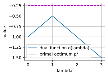
p* = -0.2500,  d* = -0.5000 at lambda = 1.00,  gap = 0.2500
weak duality q(lambda) <= p* everywhere: True
p* = -0.2500,  d* = -0.5000 at lambda = 1.00,  gap = 0.2500
weak duality q(lambda) <= p* everywhere: True
p* = -0.2500,  d* = -0.5000 at lambda = 1.00,  gap = 0.2500
weak duality q(lambda) <= p* everywhere: True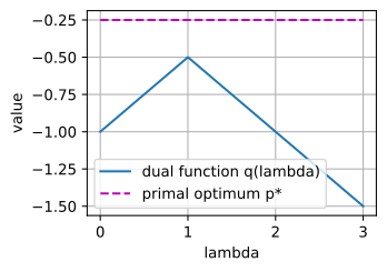
The tent-shaped dual function peaks at \(-\tfrac12\), a quarter below the primal optimum. A strictly feasible point exists (\(x = \tfrac14\) lies inside \(\mathcal{D}\) and has \(g(\tfrac14) = -\tfrac14 < 0\)), so the gap is caused by the missing convexity, not by a missing Slater point. In panel (b) of Figure 26.6.2, the image curve \(\{(u, -(u + \tfrac12)^2) : u \in [-\tfrac12, \tfrac12]\}\) bends the wrong way, and no line below \(\mathcal{A}\) passes through its point at \(u = 0\); the best one, of slope \(-1\), certifies only \(-\tfrac12\). Duals of nonconvex problems still give valid lower bounds, but the bound need not be tight. The gap also depends on how the problem is written (Exercise 5).
We can now bound a constrained optimum from below with any nonnegative multipliers, decide from convexity and one strictly feasible point that the best bound is exact, read the optimal multipliers as the prices of the constraints, and derive the dual of a quadratic program by hand. Two questions remain open. A nonconvex problem can keep a gap, so its dual bounds but does not solve it. And iterating on \(\mathbf{x}\) and \(\boldsymbol{\lambda}\) together need not converge even when a saddle point exists, which is the difficulty behind minimax training. Training a deep network is not a convex problem, but many of its subproblems are: projections, clipped updates, last-layer fits, and trust-region steps on a convex model, and everything in this section applies to them. All of it also assumed exact arithmetic; the next section asks when finite precision, rather than the algorithm, decides the answer.
26.6.6 Summary
The dual function \(q(\boldsymbol{\lambda}, \boldsymbol{\nu}) = \inf_{\mathbf{x}} \mathcal{L}\) is concave for every problem and never exceeds \(p^\star\), so each choice of multipliers \(\boldsymbol{\lambda} \succeq 0\) certifies a lower bound. For a convex problem with a strictly feasible point (Slater’s condition) the best bound is exact, and attained primal and dual optima form a saddle point of the Lagrangian. For linear constraints the dual is a conjugate, \(q(\boldsymbol{\lambda}) = -f^*(-\mathbf{A}^\top\boldsymbol{\lambda}) - \mathbf{b}^\top\boldsymbol{\lambda}\), which turns a table of conjugates into a table of duals. Under strong duality the optimal multipliers are shadow prices, with \(\lambda_i^\star = -\partial p^\star / \partial u_i\) and \(\nu_j^\star = -\partial p^\star / \partial v_j\) when \(p^\star\) is differentiable. The SVM multipliers are positive only on support vectors, the multiplier \(1/\theta\) of the power budget in water-filling is the rate gained per unit of power, and for a convex loss the weight-decay coefficient is the multiplier of a norm budget. A nonconvex problem can keep a gap, as the concave objective with \(p^\star - d^\star = \tfrac14\) shows.
26.6.7 Exercises
Conjugate pairs. Compute each conjugate from Equation 26.6.4.
- \(f(\mathbf{x}) = \lambda\|\mathbf{x}\|_1\) with \(\lambda > 0\).
- \(f(\mathbf{x}) = \tfrac12 \mathbf{x}^\top \mathbf{A} \mathbf{x}\) with \(\mathbf{A} \succ 0\). What does the Fenchel–Young inequality Equation 26.6.5 state for this pair?
- The softplus \(f(t) = \log(1 + e^t)\) on \(\mathbb{R}\). The binary cross-entropy of a logit \(t\) against a soft label \(p \in [0, 1]\) is \(\log(1 + e^t) - pt\). Use Fenchel–Young to show that it is at least the binary entropy \(H(p) = -p\log p - (1-p)\log(1-p)\), with equality exactly when \(p = 1/(1 + e^{-t})\), the sigmoid of \(t\). Write the difference as a KL divergence.
- The double well \(\phi_0(x) = (x^2 - 1)^2\) of Section 26.2.4 (the function \(\phi\) there without its tilt \(x/2\)) is not convex. Find its convex envelope \(\phi_0^{**}\) and the set on which \(\phi_0^{**} < \phi_0\).
Adapted from Boyd and Vandenberghe, Convex Optimization, Examples 3.22 and 3.26.
Maximum entropy and temperature. The entropy of a probability vector \(\mathbf{p} \in \mathbb{R}^n\) is \(H(\mathbf{p}) = -\sum_i p_i \log p_i\). This exercise derives the softmax from the constraint side.
- Maximize \(H\) subject to \(\sum_i p_i = 1\) with one Lagrange multiplier, ignoring the sign constraints \(p_i \ge 0\). Show that the only stationary point is the uniform distribution. Why does ignoring the sign constraints not change the answer?
- Fix scores \(s_1, \ldots, s_n\), not all equal, and a target \(\bar s\) strictly between \(\min_i s_i\) and \(\max_i s_i\), and add the constraint \(\sum_i p_i s_i = \bar s\). Show that the maximizer is \(\mathbf{p} = \mathrm{softmax}(\beta\mathbf{s})\) for a scalar \(\beta\) determined by the multiplier of the score constraint. Show that the mean score under \(\mathrm{softmax}(\beta\mathbf{s})\) increases strictly with \(\beta\), so that exactly one \(\beta\) meets the target.
- Let \(H^\star(\bar s)\) be the maximal entropy. Show that \(\mathrm{d}H^\star / \mathrm{d}\bar s = -\beta\), so that the multiplier prices the score constraint as the multiplier of Section 26.5.1.3 prices the offset \(b\). For which targets \(\bar s\) is \(\beta\) negative? What happens to the softmax temperature \(1/\beta\) as \(\bar s\) approaches \(\max_i s_i\)?
A dual certificate for \(\ell_1\) minimization. Basis pursuit,
\[\min_{\mathbf{x}}\; \|\mathbf{x}\|_1 \quad \textrm{subject to} \quad \mathbf{A}\mathbf{x} = \mathbf{b}, \tag{26.6.14}\]
with \(\mathbf{A} \in \mathbb{R}^{m \times n}\) and \(m < n\), selects a sparse solution of an underdetermined linear system. Its constraints are affine, so Slater’s condition in its refined form gives \(d^\star = p^\star\) whenever the system has a solution. The conjugate of \(\|\cdot\|_1\) is the indicator of the box \(\{\mathbf{y} : \|\mathbf{y}\|_\infty \le 1\}\).
- Use the equality form of Equation 26.6.6 to show that, after replacing \(\boldsymbol{\nu}\) by \(-\boldsymbol{\nu}\), the dual problem is \(\max_{\boldsymbol{\nu}} \mathbf{b}^\top \boldsymbol{\nu}\) subject to \(\|\mathbf{A}^\top \boldsymbol{\nu}\|_\infty \le 1\).
- Solve both problems by hand for \(\mathbf{A} = (1\;\; 2)\) and \(b = 2\), and check \(d^\star = p^\star\).
- Let \(\mathbf{x}^\star\) and \(\boldsymbol{\nu}^\star\) be optimal. Show that \(x_i^\star = 0\) wherever \(|(\mathbf{A}^\top \boldsymbol{\nu}^\star)_i| < 1\), and that \((\mathbf{A}^\top \boldsymbol{\nu}^\star)_i = \mathrm{sign}(x_i^\star)\) wherever \(x_i^\star \neq 0\). A candidate \(\mathbf{x}\) with \(\mathbf{A}\mathbf{x} = \mathbf{b}\) is given. Which conditions must a vector \(\boldsymbol{\nu}\) satisfy to certify that \(\mathbf{x}\) is optimal without solving the problem?
Support vectors and the dual value. For the offset-folded SVM dual Equation 26.6.12, let \(\boldsymbol{\alpha}^\star\) be optimal and \(\tilde{\mathbf{w}}^\star = \sum_i \alpha_i^\star y_i \tilde{\mathbf{x}}_i\).
- Show that \(\sum_i \alpha_i^\star = \|\tilde{\mathbf{w}}^\star\|^2\) by writing the KKT conditions of the dual over the orthant. Conclude that the dual optimal value equals the primal value \(\tfrac12 \|\tilde{\mathbf{w}}^\star\|^2\).
- Show that deleting a training point with \(\alpha_j^\star = 0\) leaves the remaining multipliers optimal for the smaller problem and leaves \(\tilde{\mathbf{w}}^\star\) unchanged. In leave-one-out validation, each of the \(n\) points is classified by the SVM trained on the other \(n - 1\) points. Conclude that the leave-one-out error rate is at most the fraction of points with \(\alpha_i^\star > 0\), for every optimal \(\boldsymbol{\alpha}^\star\). Which optimal \(\boldsymbol{\alpha}^\star\) gives the best bound?
- [code] The matrix \(\mathbf{Q}\) of the SVM cell has rank \(3\). Let \(S\) be the four indices with \(\alpha_i^\star > 0\) and \(\mathbf{G}_S\) the corresponding rows of
G. Find a nonzero \(\mathbf{d} \in \mathbb{R}^4\) with \(\mathbf{G}_S^\top\mathbf{d} = \mathbf{0}\) (usenp.linalg.svdof \(\mathbf{G}_S^\top\)), and move \(\boldsymbol{\alpha}^\star_S + t\mathbf{d}\) in each direction until a coordinate reaches zero. Verify that both endpoints are dual feasible, have dual value \(\tfrac{41}{98}\), and give the same \(\tilde{\mathbf{w}}^\star\). Which margin-\(1\) point has \(\alpha_i = 0\) at each endpoint? What does this say about reading “support vector” off the multipliers? (You should find the endpoints \((0, 0.204, 0, 0, 0, 0.192, 0, 0.441)\) and \((0.204, 0, 0, 0, 0, 0.273, 0, 0.359)\).)
[code] Duality gaps and formulations. The gap cell of Section 26.6.5.3 minimizes the Lagrangian over the domain \([0, 1]\) and dualizes only the constraint \(x \le \tfrac12\).
- Replace the objective by \(f(x) = (x - 1)^2\). Compute \(p^\star\), the dual function, \(d^\star\), and \(\lambda^\star\) by hand, and confirm them with the modified cell. Why is the gap now zero?
- Keep \(f(x) = -x^2\), but write the constraint as \(x^2 \le \tfrac14\), which defines the same feasible set on \([0, 1]\). Compute the new dual function and \(d^\star\) by hand and with the cell.
- Keep \(f(x) = -x^2\) and the constraint \(x \le \tfrac12\), but treat \(0 \le x\) and \(x \le 1\) as constraints with their own multipliers and minimize the Lagrangian over all of \(\mathbb{R}\). What is \(d^\star\) now? Rank the dual bounds of the three formulations of the same problem (the one in the text and those of the two previous parts). Is a duality gap a property of the problem or of its formulation?
[code] Gradient descent–ascent. ● Primal–dual methods and GAN training update the minimizing variable by gradient descent and the maximizing variable by gradient ascent at the same time.
- For the bilinear game \(\min_x \max_y\, xy\), whose saddle point is the origin, write simultaneous descent–ascent, \(x \leftarrow x - \eta y\) and \(y \leftarrow y + \eta x\), as a linear map. Show that every nonzero start spirals away from the saddle for every \(\eta > 0\). Show that the alternating version, in which the \(y\)-update uses the new \(x\), is a linear map with determinant \(1\). What do its iterates do for \(\eta < 2\)?
- Run simultaneous descent–ascent on the Lagrangian \(\mathcal{L}(\mathbf{x}, \nu) = \tfrac12\mathbf{x}^\top \mathbf{x} + \nu(\mathbf{a}^\top \mathbf{x} - b)\) of the closest-point problem of Section 26.5.1.3, with \(\mathbf{a} = (1, 2)\), \(b = 1\), and the start \(\mathbf{x} = \mathbf{0}\), \(\nu = 0\). Find the step sizes for which the iterates converge to \((\mathbf{x}^\star, \nu^\star)\). Derive them from the eigenvalues of the update acting on the pair \((\mathbf{a}^\top \mathbf{x} / \|\mathbf{a}\|, \nu)\) and on the components of \(\mathbf{x}\) orthogonal to \(\mathbf{a}\).
- Add \(\tfrac{\epsilon}{2} x^2\) with \(0 < \epsilon \le 2\) to the objective of the bilinear game. For which step sizes does simultaneous descent–ascent converge now? Which term of the Lagrangian of the previous part plays the role of \(\epsilon\)?
[code] Penalty versus constraint without convexity. ● For a convex loss, Section 26.6.4.2 shows that weight decay and a norm constraint trace the same solutions. Take instead the nonconvex one-dimensional loss \(\ell(w) = (w - 1)^2 (w - 3)^2 - w\), whose local minima lie near \(w = 1.16\) and \(w = 3.11\).
- On a fine grid of \(w\), compute the penalized minimizers \(w_\lambda = \mathrm{argmin}_w\, \ell(w) + \tfrac\lambda2 w^2\) for \(\lambda\) on a logarithmic grid, and the constrained optimum \(p^\star(r) = \min \{\ell(w) : w^2 \le r^2\}\) for \(r \in [0, 3.2]\). Plot the points \((w_\lambda^2, \ell(w_\lambda))\) on top of the curve \((r^2, p^\star(r))\). Which budgets \(r\) are never the norm \(|w_\lambda|\) of a penalized minimizer?
- Show that \(w_\lambda\) minimizes \(\ell(w) + \tfrac\lambda2 w^2\) if and only if the line of slope \(-\tfrac\lambda2\) through \((w_\lambda^2, \ell(w_\lambda))\) lies below every point of the set \(\{(w^2, \ell(w)) : w \in \mathbb{R}\}\). Use this and the supporting-line picture of Figure 26.6.2 to explain the missing budgets.
- Pick a budget \(r\) in the missing range at which the constraint is active. Compute the KKT multiplier \(\lambda\) of the constrained solution, with the constraint written \(\tfrac12 w^2 \le \tfrac12 r^2\) as in the text, and find a point where the penalized objective with this \(\lambda\) is lower. Compute the duality gap \(p^\star(r) - d^\star(r)\) of the constrained problem.
[extended] Entropic optimal transport. ●● Given probability vectors \(\mathbf{p} \in \mathbb{R}^n\) and \(\mathbf{r} \in \mathbb{R}^m\) and a cost matrix \(\mathbf{C} \in \mathbb{R}^{n \times m}\), optimal transport finds the cheapest plan \(\boldsymbol{\Gamma}\) that moves the mass \(\mathbf{p}\) to the mass \(\mathbf{r}\),
\[\mathrm{OT} = \min_{\boldsymbol{\Gamma} \ge 0}\; \sum_{i,j} C_{ij} \Gamma_{ij} \quad \textrm{subject to} \quad \boldsymbol{\Gamma} \mathbf{1} = \mathbf{p}, \;\; \boldsymbol{\Gamma}^\top \mathbf{1} = \mathbf{r}, \tag{26.6.15}\]
a linear program with \(nm\) variables. Entropic regularization (Cuturi 2013) adds \(\varepsilon \sum_{i,j} \Gamma_{ij} (\log \Gamma_{ij} - 1)\) to the objective, with \(\varepsilon > 0\); let \(\boldsymbol{\Gamma}_\varepsilon\) be the regularized optimum. Its solution by Sinkhorn iterations is used to compare distributions (Peyré and Cuturi 2019).
Form the Lagrangian with the terms \(\boldsymbol{\phi}^\top (\mathbf{p} - \boldsymbol{\Gamma} \mathbf{1}) + \boldsymbol{\psi}^\top (\mathbf{r} - \boldsymbol{\Gamma}^\top \mathbf{1})\) for the marginal constraints. Show that \(\boldsymbol{\Gamma}_\varepsilon = \mathrm{diag}(\mathbf{u})\, \mathbf{K}\, \mathrm{diag}(\mathbf{v})\) with \(K_{ij} = e^{-C_{ij} / \varepsilon}\), \(u_i = e^{\phi_i / \varepsilon}\), and \(v_j = e^{\psi_j / \varepsilon}\). Why can the sign constraints \(\Gamma_{ij} \ge 0\) be left out of the Lagrangian?
Show that the dual function is
\[q(\boldsymbol{\phi}, \boldsymbol{\psi}) = \mathbf{p}^\top \boldsymbol{\phi} + \mathbf{r}^\top \boldsymbol{\psi} - \varepsilon \sum_{i,j} e^{(\phi_i + \psi_j - C_{ij}) / \varepsilon}, \tag{26.6.16}\]
and that maximizing it exactly over \(\boldsymbol{\phi}\) with \(\boldsymbol{\psi}\) fixed gives the Sinkhorn update \(\mathbf{u} = \mathbf{p} / (\mathbf{K} \mathbf{v})\), elementwise. Conclude that Sinkhorn’s algorithm is block-coordinate ascent on a concave function and that its dual value never decreases. Why is every dual value a lower bound on \(\mathrm{OT}\)?
Let \(H(\boldsymbol{\Gamma}) = -\sum_{i,j} \Gamma_{ij} \log \Gamma_{ij}\), and grant that every feasible plan satisfies \(\max(H(\mathbf{p}), H(\mathbf{r})) \le H(\boldsymbol{\Gamma}) \le H(\mathbf{p}) + H(\mathbf{r})\). Show that \(0 \le \sum_{i,j} C_{ij} (\boldsymbol{\Gamma}_\varepsilon)_{ij} - \mathrm{OT} \le \varepsilon \min(H(\mathbf{p}), H(\mathbf{r}))\).
Let the costs lie in \([0, 1]\). In float64, \(e^{-x}\) rounds to zero for \(x\) above about \(745\). For which \(\varepsilon\) can entries of \(\mathbf{K}\) vanish, and what then happens to the multiplicative updates \(\mathbf{u} = \mathbf{p} / (\mathbf{K}\mathbf{v})\)? Explain why updating \(\boldsymbol{\phi}\) and \(\boldsymbol{\psi}\) directly, with a log-sum-exp in place of the products with \(\mathbf{K}\), avoids the problem.
[code] The dual of ridge regression. Write \(\min_{\mathbf{w}}\tfrac12\|\mathbf{A}\mathbf{w} - \mathbf{b}\|^2 + \tfrac\lambda2\|\mathbf{w}\|^2\), with \(\mathbf{A} \in \mathbb{R}^{n \times d}\), as \(\min_{\mathbf{w}, \mathbf{z}}\tfrac12\|\mathbf{z}\|^2 + \tfrac\lambda2\|\mathbf{w}\|^2\) subject to \(\mathbf{A}\mathbf{w} - \mathbf{b} - \mathbf{z} = \mathbf{0}\), with multiplier \(\boldsymbol{\alpha} \in \mathbb{R}^n\).
- Minimize the Lagrangian over \(\mathbf{z}\) and \(\mathbf{w}\) to get \(\mathbf{z} = \boldsymbol{\alpha}\), \(\mathbf{w} = -\mathbf{A}^\top\boldsymbol{\alpha}/\lambda\), and the dual function \(q(\boldsymbol{\alpha}) = -\tfrac12\|\boldsymbol{\alpha}\|^2 - \tfrac1{2\lambda}\boldsymbol{\alpha}^\top\mathbf{A}\mathbf{A}^\top\boldsymbol{\alpha} - \mathbf{b}^\top\boldsymbol{\alpha}\). Why does strong duality hold?
- Maximize \(q\) to get \(\boldsymbol{\alpha}^\star = -\lambda(\mathbf{A}\mathbf{A}^\top + \lambda\mathbf{I})^{-1}\mathbf{b}\) and \(\mathbf{w}^\star = \mathbf{A}^\top(\mathbf{A}\mathbf{A}^\top + \lambda\mathbf{I})^{-1}\mathbf{b}\). Explain why the solution is a combination of the rows of \(\mathbf{A}\), as the SVM weight vector is a combination of the data points, and why the data enter only through \(\mathbf{A}\mathbf{A}^\top\).
- For \(n = 20\) examples and \(d = 50\) features, verify numerically that the primal solve \((\mathbf{A}^\top\mathbf{A} + \lambda\mathbf{I})\mathbf{w} = \mathbf{A}^\top\mathbf{b}\) and the dual formula agree to about \(10^{-14}\), and that the primal and dual values coincide. Which solve is cheaper when \(n \ll d\)? What does replacing \(\mathbf{A}\mathbf{A}^\top\) by a kernel matrix give?
[code] Dual ascent and the gradient of the dual. For the clipping problem, \(q(\lambda) = \tfrac{25}{2}\tfrac{\lambda}{1 + \lambda} - \tfrac\lambda2\) and the Lagrangian’s minimizer is \(\mathbf{x}(\lambda) = \mathbf{x}_0 / (1 + \lambda)\).
- Show that \(q'(\lambda) = g(\mathbf{x}(\lambda))\). Explain why the same holds for any problem whose Lagrangian has a unique minimizer \(\mathbf{x}(\boldsymbol{\lambda})\) that depends smoothly on \(\boldsymbol{\lambda}\): differentiate \(q(\boldsymbol{\lambda}) = \mathcal{L}(\mathbf{x}(\boldsymbol{\lambda}), \boldsymbol{\lambda})\) and use stationarity to drop the term through \(\mathbf{x}\). The gradient of the dual is the vector of constraint values at the Lagrangian’s minimizer.
- Run projected dual ascent, \(\lambda \leftarrow \max\bigl(0, \lambda + \eta\, g(\mathbf{x}(\lambda))\bigr)\), from \(\lambda = 0\) with \(\eta \in \{0.5, 1, 2\}\), and report the iterate after \(10\), \(50\), and \(100\) steps. (For \(\eta = 0.5\) you should see about \(5.07\), \(4.02\), and \(4.0001\).) The first step jumps to \(12\eta\), far past \(\lambda^\star = 4\). Explain this from \(q''(\lambda) = -25/(1 + \lambda)^3\), which is \(-25\) at \(\lambda = 0\) and \(-0.2\) at \(\lambda = 4\). Why does a step size that is safe near \(\lambda^\star\) jump so far at the start?
- For \(\eta = 0.5\), are the points \(\mathbf{x}(\lambda_k)\) feasible? Show that every feasible \(\mathbf{x}(\lambda_k)\) gives an upper bound \(f(\mathbf{x}(\lambda_k)) \ge p^\star\) while \(q(\lambda_k)\) gives a lower bound, and print the certified gap \(f(\mathbf{x}(\lambda_k)) - q(\lambda_k)\) along the run. Relate dual ascent to the Sinkhorn updates of Exercise 8, which maximize the same kind of dual exactly in blocks.
The chapter’s quadratic against a half-plane. Minimize \(\tfrac12(x_1^2 + 1000\,x_2^2)\) subject to \(x_1 + x_2 \ge 1\).
- Write the constraint as \(-x_1 - x_2 \le -1\) and use Equation 26.6.6 with the conjugate of \(\tfrac12\mathbf{x}^\top\mathbf{A}\mathbf{x}\) from Exercise 1b to get \(q(\lambda) = \lambda - \tfrac12\lambda^2(1 + \tfrac1{1000})\). Find \(\lambda^\star = \tfrac{1000}{1001}\), \(p^\star = d^\star = \tfrac{500}{1001} \approx 0.4995\), and \(\mathbf{x}^\star = (0.999, 0.000999)\).
- Why does \(x_2^\star\) carry almost none of the constraint? By how much, to first order, does the optimum rise if the constraint becomes \(x_1 + x_2 \ge 1 + \delta\)?
- Replace \(1000\) by a curvature ratio \(\kappa\) and let \(\kappa \to \infty\). What do \(\lambda^\star\), \(p^\star\), and \(\mathbf{x}^\star\) tend to? Fixed-step gradient descent on the unconstrained quadratic slows down by a factor of about \(\kappa\) (Section 26.1). Does the ill-conditioning make this constrained problem hard to solve through its dual?