%matplotlib inline
from d2l import torch as d2l
import math
import numpy as np
import torch
from torch import nn
import torch.nn.functional as F12.7 Hybrid Architectures
The preceding sections improve how a fixed-size state stores information, but do not change its finite capacity. Exact recall over an unbounded context therefore remains impossible. A hybrid architecture combines the constant-memory behavior of recurrent layers with the exact retrieval of a smaller number of attention layers.
This section first states a counting bound for fixed-state recall and then compares the cache cost of recurrent and attention layers. Three matched models isolate the effect of inserting one attention layer into a recurrent stack. We conclude with design patterns reported for deployed hybrids and with methods for distilling a pretrained transformer into a hybrid model.
Prerequisites: the KV-cache accounting of Section 11.3 (Equation 11.3.1); the matrix state, its capacity proposition, and the duality of Section 12.4; and the recall task of Section 12.5.1.1.
%matplotlib inline
from d2l import jax as d2l
from flax import nnx
import jax
from jax import numpy as jnp
import math
import numpy as np
import optax
12.7.1 What a Fixed State Cannot Do
Selectivity makes recurrent updates content-dependent. The delta rule replaces additive writes with corrective writes, and test-time learning updates the state from recent observations. None of these changes increases the capacity of a fixed-size state. At any fixed numerical precision, a state of \(N\) numbers holds a bounded number of bits. To reproduce \(k\) arbitrary tokens from a vocabulary of size \(V\), something in the model must hold \(k \log_2 V\) bits from the moment they appear to the moment they are needed. Our own measurements have analyzed this limitation throughout the chapter. The crowding proposition of Section 12.4.1.1 quantifies one aspect: expected squared read error \((n-1)/d_k\) after \(n\) random-key writes, interference growing linearly in how much you store. The transition comparison in Table 12.5.1 addresses another aspect: each row changes what the state can compute — forgetting, erasure, reflections, group words — while the number of bits it holds never moved.
Jelassi et al. (2024) make the limit a theorem, using the purest recall task there is: copying. Both directions of their comparison carry conditions, so we state the two results together, with matching quantifiers.
The copy bounds (Jelassi et al. 2024). Transformer, upper bound: there is a depth-two transformer of width \(O(n \log D)\) that copies any string over an alphabet of size \(D\) up to length \(D^n\), provided no length-\(n\) substring repeats — the construction addresses the archive by hashed \(n\)-grams, and the attention window over everything so far supplies the storage, growing with the sequence. Generalized SSM, lower bound: any model that pushes the sequence through a fixed, finite state set \(\mathcal{S}\) — every architecture in this chapter, at any fixed precision — errs on copying a string drawn uniformly at random from the \(D^L\) strings of length \(L\) with probability at least \(1 - |\mathcal{S}|/D^L\); once the state holds fewer than about \(L \log_2 D\) bits, it gets most such copies wrong.
Neither half reduces to “attention remembers, recurrence cannot”. The upper bound is a construction, valid for strings without repeated \(n\)-grams; the lower bound is a counting argument over the uniform copy distribution, and it says nothing about a narrower workload — a state that stores just the strings its training distribution favors evades it. What the count does rule out is a fixed state that copies arbitrary strings much longer than its bit budget: there are \(D^L\) required outputs and only \(|\mathcal{S}|\) states to route them through, and no parameterization, gating, or training trick appears anywhere in that ratio. Empirically the crossover is not close: on synthetic phone-book lookup, their smallest transformer (410M parameters) beats a 2.8B-parameter Mamba once the book exceeds roughly seventy entries.
How does this capacity limit affect language tasks? Arora, Eyuboglu, Timalsina, et al. (2024) located it with multi-query associative recall (MQAR): a stream writes key–value bindings, later re-presents keys in arbitrary order, and the model must produce each key’s value — our overwrite task of Section 12.5.1.1, embedded in text. Across seventeen trained language models, 82% of the perplexity gap between efficient architectures and attention fell on the recall slice — the tokens whose prediction requires retrieving a binding seen once before. Attention solves MQAR at a width independent of sequence length; recurrent models solve it only while the bindings in play fit in their state — the crowding picture again, now diagnosed in the wild.
At production scale the failure has a name. In NVIDIA’s controlled 8B-parameter comparison, a pure Mamba-2 model matched a transformer on perplexity and most benchmarks while scoring 29% on five-shot MMLU against the transformer’s 46%, and its phone-book recall collapsed once the book grew past a few hundred tokens; the authors call the mode fuzzy memory — the model returns an answer that shares digits with the right one (Waleffe et al. 2024). Ablating the few full-attention layers of a deployed hybrid reduces needle-in-a-haystack retrieval to roughly zero. A small number of full-attention layers provides retrieval, whereas the linear-recurrent majority provides less expensive throughput.
Gu (2025) describes the trade in terms of compressed and uncompressed memory. A recurrent state compresses the preceding sequence into a fixed-size representation and must determine at write time which information to retain. A transformer’s key–value cache instead stores a separate representation for every retained token, preserving exact retrieval at a cost that grows with context length. Hybrid architectures combine these complementary memory mechanisms.
12.7.2 Inference-Memory Cost
A pure transformer preserves recall but incurs the cache cost measured in Section 11.3: cache bytes \(= 2 \cdot n_\textrm{layers} \cdot n_\textrm{kv} \cdot d_\textrm{head} \cdot n \cdot b\) times the element size, Equation 11.3.1, growing linearly in the context length \(n\). The factor that matters here is \(n_\textrm{layers}\): the cache is paid per attention layer. A recurrent layer holds a state whose shape Equation 12.4.1 fixes at \(d_k \times d_v\) numbers per head and whose bytes the per-layer formula Equation 12.4.7 prices. Priced concretely, a Mamba-2 layer at \(d_\textrm{model} = 4096\) with the usual expansion factor of two (so \(d_\textrm{inner} = 8192\)) and state width \(d_\textrm{state} = 128\) carries \(8192 \cdot 128 \approx 1.05\textrm{M}\) state elements — about 2 MB at the fp16 serving precision that formula’s headline uses, with the small convolution buffer adding another two percent — and that figure is the same at token one hundred and at token one million. A full-attention layer with grouped queries at the same width pays 4 KB per token: past a few hundred tokens the growing archive dwarfs the flat state, and by 128K context one attention layer holds 512 MB against the recurrent layer’s 2 MB. Figure 12.7.1 draws the consequence for a whole model: replacing most attention layers with recurrent ones reduces persistent memory by almost exactly the removed attention fraction, because only the surviving attention layers retain a context-dependent cache.
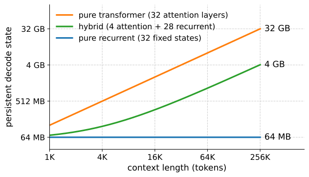
Those curves are not hypothetical: they are the memory column of Jamba’s model card. At 256K context, Jamba — 4 attention layers out of 32, the rest Mamba — reports a 4 GB key–value cache where the comparably sized Mixtral carries 32 GB and a Llama-2-70B-class transformer 128 GB (Lieber et al. 2024). An eightfold saving on the resource that decides how many concurrent users fit on an accelerator is the kind of number that redraws architectures, and it follows from the layer count in Equation 11.3.1. (Recall from Section 11.3 that decode is bandwidth-bound, so cache bytes are also the currency of generation speed.)
One structural remark before we measure the other side of the trade. The cache relief of Section 11.3 came in flavors that compose: GQA and MLA shrink the width of each cached token, sliding windows bound its lifetime, quantization shrinks its bytes, and a deployment can apply all three to the same cache. Replacing attention with recurrence removes the growing term rather than shrinking it. The recurrent state is a tensor like any other — it can be quantized or held in lower precision too — but it is already constant in context length, so there is no growth left to attack; the contrast that matters is not compressible-versus-not but what grows with context and what does not. A hybrid gets both moves: the recurrent majority contributes only constant state, and the attention minority keeps a cache that GQA, MLA, and quantization still shrink (the recipe table below shows shipped hybrids doing exactly this). The remaining quantitative question is how few attention layers a model can retain while preserving transformer-like recall.
12.7.3 Recall with One Attention Layer
We answer at teaching scale, with machinery this book has already built. Three models, identical in every dimension — depth, width, heads, embeddings, MLPs, parameter count to within a percent (the model cell below prints the counts) — except for the token mixer inside each block. The task is MQAR, sized so that the sweep crosses the fixed state’s capacity. The claim to test is the one the last two sections set up: recall should collapse for the pure recurrent stack when the bindings exceed what its state can hold, a single mid-stack attention layer should restore it, and language-model loss should barely notice any of it.
12.7.3.1 Three Matched Models
The task generator is the one from Section 12.5.1.1 with the re-binding knob removed and the load knob exposed: each sequence writes num_pairs distinct key–value bindings, then queries every key in random order. Sweeping num_pairs sweeps the number of bits the model must carry from write phase to query phase.
def make_recall(num_seqs, num_pairs, num_keys=64, num_values=32, seed=0):
    """Write num_pairs distinct bindings, then query each key once."""
    task_rng = np.random.default_rng(seed)
    P, T = num_pairs, 2 * num_pairs
    QUERY = num_values                    # A reserved "query" content token
    keys = np.zeros((num_seqs, T), np.int64)
    vals = np.full((num_seqs, T), QUERY, np.int64)
    tgt = np.full((num_seqs, T), -1, np.int64)
    for b in range(num_seqs):
        ks = task_rng.choice(num_keys, size=P, replace=False)
        vs = task_rng.integers(0, num_values, size=P)
        keys[b, :P], vals[b, :P] = ks, vs
        qorder = task_rng.permutation(P)
        keys[b, P:] = ks[qorder]
        tgt[b, P:] = vs[qorder]
    return keys, vals, tgt                # tgt = -1 outside the query phase
def make_recall(num_seqs, num_pairs, num_keys=64, num_values=32, seed=0):
"""Write num_pairs distinct bindings, then query each key once."""
task_rng = np.random.default_rng(seed)
P, T = num_pairs, 2 * num_pairs
QUERY = num_values # A reserved "query" content token
keys = np.zeros((num_seqs, T), np.int64)
vals = np.full((num_seqs, T), QUERY, np.int64)
tgt = np.full((num_seqs, T), -1, np.int64)
for b in range(num_seqs):
ks = task_rng.choice(num_keys, size=P, replace=False)
vs = task_rng.integers(0, num_values, size=P)
keys[b, :P], vals[b, :P] = ks, vs
qorder = task_rng.permutation(P)
keys[b, P:] = ks[qorder]
tgt[b, P:] = vs[qorder]
return keys, vals, tgt # tgt = -1 outside the query phaseThe recurrent mixer is scalar-gated linear attention: an input-dependent decay \(a_t\), one number per head per token, applied to a matrix state per head. On the decay ladder of Figure 12.4.1 this is Mamba-2’s rung (Dao and Gu 2024), one below the per-coordinate diagonal gate that defines GLA proper (Yang et al. 2024); we take the scalar rung because it is the cheapest transition that forgets, and name the class for what it is: ScalarGatedMixer. We train it through the quadratic dual \(\mathbf{Y} = (\mathbf{L} \circ
\mathbf{Q}\mathbf{K}^\top)\mathbf{V}\) of Equation 12.4.6, which Section 12.4.2 verified equal to the recurrence to float32 rounding — so this is a genuine linear-recurrence model, computed the fast way.
Three implementation details determine whether the comparison is valid. First, initialize a new gate to retain information. With a default-initialized gate the decay comes out around \(a \approx 0.5\) per token — a state half-life of one token — and the untrained model destroys the write phase before the query phase arrives; it then sits at chance recall for every load we test, and training rarely digs it out. Initializing the gate bias at \(-4.5\) gives \(a \approx 0.99\), a half-life of about seventy tokens, and the problem disappears. Every production cell in this family makes the same move: S4D’s small initial step sizes (Section 12.2.5), Mamba’s \(\Delta\) bias, the retention bias we gave Gated DeltaNet in Section 12.5.4. Second, mask before exponentiating. The dual builds \(\mathbf{L}\) as \(\exp(\textrm{cum}_i - \textrm{cum}_j)\); above the diagonal that exponent is large and positive, and once training pushes some head’s decay toward zero — which language modeling does within a few hundred steps — the \(\exp\) overflows to infinity and inf * 0 = nan kills the run. Masking with \(-\infty\) before the \(\exp\), as segsum did in Section 12.4.3, makes the upper triangle an exact zero instead. In our runs the recall task does not trigger this overflow; the language-modeling panel below does, reliably. A bug that only fires on one of your two benchmarks is the expensive kind. Third, normalize the read-out. The memory read \(\mathbf{S}_t^\top
\mathbf{q}_t\) is a sum over everything the state has accumulated, so its scale grows with how much has been written — order \(\sqrt{T}\) at initialization — while the residual stream it joins does not. This family therefore normalizes the output, not a carried normalizer state (the design decision discussed in Section 12.4, and the RMSNorm inside our Gated DeltaNet cell): a per-head RMSNorm on the read-out before the output projection. Without it, our four-block stacks train erratically at this sequence length — in one framework the hybrid never leaves chance recall — because the untrained recurrent-block outputs dominate the residual stream, preventing the downstream attention layer from recovering the tokens.
class ScalarGatedMixer(nn.Module):
    """Scalar-gated linear attention (Mamba-2's rung), via the dual."""
    def __init__(self, num_hiddens, num_heads):
        super().__init__()
        self.num_heads, self.d_head = num_heads, num_hiddens // num_heads
        self.W_qkv = nn.Linear(num_hiddens, 3 * num_hiddens, bias=False)
        self.W_g = nn.Linear(num_hiddens, num_heads)
        nn.init.constant_(self.W_g.bias, -4.5)     # A fresh gate must retain
        self.norm = nn.RMSNorm(self.d_head)        # Normalize the read-out
        self.W_o = nn.Linear(num_hiddens, num_hiddens, bias=False)

    def forward(self, X, *_):
        B, T, d = X.shape
        q, k, v = self.W_qkv(X).reshape(B, T, self.num_heads, 3,
                                        self.d_head).unbind(3)
        log_a = -F.softplus(self.W_g(X))           # log a_t < 0, per head
        cum = log_a.cumsum(1)
        logL = cum[:, :, None, :] - cum[:, None, :, :]   # (B, T, T, heads)
        causal = torch.tril(torch.ones(T, T, dtype=torch.bool,
                                       device=X.device))
        logL = logL.masked_fill(~causal[None, :, :, None], -torch.inf)
        scores = torch.einsum('bihd,bjhd->bijh', q, k) / math.sqrt(self.d_head)
        Y = torch.einsum('bijh,bjhd->bihd', torch.exp(logL) * scores, v)
        return self.W_o(self.norm(Y).reshape(B, T, d))
class ScalarGatedMixer(nnx.Module):
"""Scalar-gated linear attention (Mamba-2's rung), via the dual."""
def __init__(self, num_hiddens, num_heads, rngs=None):
rngs = nnx.Rngs(0) if rngs is None else rngs
self.num_heads, self.d_head = num_heads, num_hiddens // num_heads
self.W_qkv = nnx.Linear(num_hiddens, 3 * num_hiddens, use_bias=False,
rngs=rngs)
self.W_g = nnx.Linear(num_hiddens, num_heads, rngs=rngs,
bias_init=nnx.initializers.constant(-4.5))
self.norm = nnx.RMSNorm(self.d_head, rngs=rngs) # Normalize read-out
self.W_o = nnx.Linear(num_hiddens, num_hiddens, use_bias=False,
rngs=rngs)
def __call__(self, X, *_):
B, T, d = X.shape
qkv = self.W_qkv(X).reshape(B, T, self.num_heads, 3, self.d_head)
q, k, v = qkv[..., 0, :], qkv[..., 1, :], qkv[..., 2, :]
log_a = -jax.nn.softplus(self.W_g(X)) # log a_t < 0, per head
cum = jnp.cumsum(log_a, 1)
logL = cum[:, :, None, :] - cum[:, None, :, :] # (B, T, T, heads)
causal = jnp.tril(jnp.ones((T, T), bool))
logL = jnp.where(causal[None, :, :, None], logL, -jnp.inf)
scores = jnp.einsum('bihd,bjhd->bijh', q, k) / math.sqrt(self.d_head)
Y = jnp.einsum('bijh,bjhd->bihd', jnp.exp(logL) * scores, v)
return self.W_o(self.norm(Y).reshape(B, T, d)), NoneThe attention mixer needs no new code at all: it is the causal multi-head attention of Section 11.2, dropped into the configurable block of Section 11.1 through its attn_factory hook — the same hook the GPT model itself uses. A stack is then a string: one letter per block, 'G' for the scalar-gated recurrence, 'A' for full attention. The entire architectural question of this section fits in three such strings.
LAYOUTS = {'linear': 'GGGG', 'attention': 'AAAA', 'hybrid': 'GGAG'}LAYOUTS = {'linear': 'GGGG', 'attention': 'AAAA', 'hybrid': 'GGAG'}The hybrid places its one attention layer third of four — mid-stack, not first, a choice the design rules below will justify. Everything around the mixers (pre-norm residuals, MLPs, embeddings, readout) is identical across the three models; the key and value channels are embedded separately and summed, as in Section 12.5.1.1, plus a learned position embedding shared by all three (a pos=False switch drops it, and a guard in forward refuses sequences longer than the table — the exercise on attention placement relies on both).
def make_blocks(layout, num_hiddens, num_heads):
    """'G' = scalar-gated recurrence block, 'A' = full-attention block."""
    gated = lambda: ScalarGatedMixer(num_hiddens, num_heads)
    attn = lambda: d2l.GPT.CausalAttention(num_hiddens, num_heads)
    return nn.ModuleList([
        d2l.TransformerBlock(num_hiddens, num_heads, norm='layer', act='gelu',
                             attn_factory=attn if c == 'A' else gated)
        for c in layout])

class RecallModel(nn.Module):
    def __init__(self, layout, num_keys, num_values, max_len,
                 num_hiddens=32, num_heads=4, pos=True):
        super().__init__()
        self.key_emb = nn.Embedding(num_keys, num_hiddens)
        self.val_emb = nn.Embedding(num_values + 1, num_hiddens)
        self.pos_emb = nn.Embedding(max_len, num_hiddens) if pos else None
        self.blocks = make_blocks(layout, num_hiddens, num_heads)
        self.norm = nn.LayerNorm(num_hiddens)
        self.head = nn.Linear(num_hiddens, num_values)

    def forward(self, keys, vals):
        X = self.key_emb(keys) + self.val_emb(vals)
        if self.pos_emb is not None:
            assert keys.shape[1] <= self.pos_emb.num_embeddings, \
                'sequence exceeds the position table: raise max_len'
            X = X + self.pos_emb(torch.arange(keys.shape[1],
                                              device=keys.device))
        for blk in self.blocks:
            X = blk(X)
        return self.head(self.norm(X))

for name, layout in LAYOUTS.items():
    model = RecallModel(layout, num_keys=64, num_values=32, max_len=128)
    print(f'{name:>10}: '
          f'{sum(p.numel() for p in model.parameters()):,} parameters')
linear: 58,544 parameters
attention: 57,984 parameters
hybrid: 58,404 parametersdef make_blocks(layout, num_hiddens, num_heads, rngs):
"""'G' = scalar-gated recurrence block, 'A' = full-attention block."""
gated = lambda rngs: ScalarGatedMixer(num_hiddens, num_heads, rngs=rngs)
attn = lambda rngs: d2l.GPT.CausalAttention(num_hiddens, num_heads,
rngs=rngs)
return nnx.List([
d2l.TransformerBlock(num_hiddens, num_heads, norm='layer', act='gelu',
attn_factory=attn if c == 'A' else gated,
rngs=rngs)
for c in layout])
class RecallModel(nnx.Module):
def __init__(self, layout, num_keys, num_values, max_len,
num_hiddens=32, num_heads=4, pos=True, rngs=None):
rngs = nnx.Rngs(0) if rngs is None else rngs
self.key_emb = nnx.Embed(num_keys, num_hiddens, rngs=rngs)
self.val_emb = nnx.Embed(num_values + 1, num_hiddens, rngs=rngs)
self.pos_emb = nnx.Embed(max_len, num_hiddens, rngs=rngs) \
if pos else None
self.blocks = make_blocks(layout, num_hiddens, num_heads, rngs)
self.norm = nnx.LayerNorm(num_hiddens, rngs=rngs)
self.head = nnx.Linear(num_hiddens, num_values, rngs=rngs)
def __call__(self, keys, vals):
X = self.key_emb(keys) + self.val_emb(vals)
if self.pos_emb is not None:
assert keys.shape[1] <= self.pos_emb.num_embeddings, \
'sequence exceeds the position table: raise max_len'
X = X + self.pos_emb(jnp.arange(keys.shape[1]))
for blk in self.blocks:
X = blk(X)
return self.head(self.norm(X))
for name, layout in LAYOUTS.items():
model = RecallModel(layout, num_keys=64, num_values=32, max_len=128,
rngs=nnx.Rngs(0))
n_params = sum(x.size for x in
jax.tree.leaves(nnx.state(model, nnx.Param)))
print(f'{name:>10}: {n_params:,} parameters') linear: 58,544 parameters
attention: 57,984 parameters
hybrid: 58,404 parametersThe printed counts back the “matched” claim with numbers: 58,544 (linear), 57,984 (attention), and 58,404 (hybrid) parameters — a spread of 560, just under one percent, coming from the gate projection and read-out norm that each scalar-gated mixer carries and the attention mixer does not. Parameter count is not sufficient for a fair comparison (the mixers do different amounts of compute per token, which Table 12.7.2 prices), but it rules out the crudest confound: none of the recall differences below can come from a larger model.
12.7.3.2 The Recall Sweep
Width is the experiment’s one carefully chosen number. At num_hiddens=32 with four heads, each head’s state is \(8 \times 8\). The random-key proposition of Section 12.4.1.1 suggests a head crowds at order-eight bindings, so a sweep of num_pairs from 4 to 64 should cross the whole stack’s capacity mid-sweep. Treat that as a sizing heuristic, not as the theory of this model: a trained four-layer stack with learned keys is far from the proposition’s single random-key memory. (Widen the model and the cliff should move right; the counting bound above says it cannot disappear.) One protocol note: small-scale MQAR results are notoriously sensitive to the learning rate, so Arora, Eyuboglu, Timalsina, et al. (2024) sweep it per configuration and report the best. We piloted their grid \(\{3 \times 10^{-4}, 10^{-3}, 3 \times 10^{-3}\}\) and pin the winner, \(3 \times 10^{-3}\), for every cell below; at \(3 \times 10^{-4}\), every architecture sits near chance at the largest loads, and a careless single-rate comparison at that setting would report no architecture gap at all. The learning rate can create or obscure the architecture gap. We therefore select it with a pilot sweep and report the fixed value used below.
def train_recall(layout, num_pairs, lr=3e-3, num_keys=64, num_values=32,
                 epochs=16, batch_size=128):
    device = d2l.try_gpu()
    torch.manual_seed(0)
    num_train = 8192 if num_pairs <= 16 else 16384
    data = [torch.tensor(x, device=device) for x in
            make_recall(num_train, num_pairs, num_keys, num_values, seed=1)
            + make_recall(2048, num_pairs, num_keys, num_values, seed=2)]
    Xk, Xv, y, Vk, Vv, Vy = data
    model = RecallModel(layout, num_keys, num_values,
                        2 * num_pairs).to(device)
    opt = torch.optim.Adam(model.parameters(), lr=lr)
    for epoch in range(epochs):
        for i in torch.randperm(num_train, device=device).split(batch_size):
            loss = F.cross_entropy(
                model(Xk[i], Xv[i]).reshape(-1, num_values),
                y[i].reshape(-1), ignore_index=-1)
            opt.zero_grad(); loss.backward(); opt.step()
    with torch.no_grad():
        pred, mask = model(Vk, Vv).argmax(-1), Vy != -1
        return float((pred[mask] == Vy[mask]).float().mean())

loads = [4, 8, 16, 32, 64]
recall = {name: [train_recall(layout, P) for P in loads]
          for name, layout in LAYOUTS.items()}
print(f"{'pairs':>10}" + ''.join(f'{P:>7}' for P in loads))
for name, accs in recall.items():
    print(f'{name:>10}' + ''.join(f'{a:>7.3f}' for a in accs))
print(f"{'chance':>10}" + f'{1 / 32:>7.3f}' * len(loads))
pairs 4 8 16 32 64
linear 0.991 0.976 0.934 0.888 0.301
attention 1.000 1.000 1.000 1.000 1.000
hybrid 1.000 1.000 1.000 1.000 1.000
chance 0.031 0.031 0.031 0.031 0.031def train_recall(layout, num_pairs, lr=3e-3, num_keys=64, num_values=32,
epochs=16, batch_size=128):
num_train = 8192 if num_pairs <= 16 else 16384
Xk, Xv, y = map(jnp.array, make_recall(num_train, num_pairs, num_keys,
num_values, seed=1))
Vk, Vv, Vy = map(jnp.array, make_recall(2048, num_pairs, num_keys,
num_values, seed=2))
model = RecallModel(layout, num_keys, num_values, 2 * num_pairs,
rngs=nnx.Rngs(0))
optimizer = nnx.Optimizer(model, optax.adam(lr), wrt=nnx.Param)
@nnx.jit
def train_step(model, optimizer, keys, vals, tgt):
def loss_fn(model):
mask = tgt != -1
losses = optax.softmax_cross_entropy_with_integer_labels(
model(keys, vals), jnp.where(mask, tgt, 0))
return (losses * mask).sum() / mask.sum()
loss, grads = nnx.value_and_grad(loss_fn)(model)
optimizer.update(model, grads)
return loss
perm_rng = np.random.default_rng(0)
for epoch in range(epochs):
for i in np.split(perm_rng.permutation(num_train),
num_train // batch_size):
train_step(model, optimizer, Xk[i], Xv[i], y[i])
pred, mask = model(Vk, Vv).argmax(-1), Vy != -1
return float((jnp.where(mask, pred == Vy, False)).sum() / mask.sum())
loads = [4, 8, 16, 32, 64]
recall = {name: [train_recall(layout, P) for P in loads]
for name, layout in LAYOUTS.items()}
print(f"{'pairs':>10}" + ''.join(f'{P:>7}' for P in loads))
for name, accs in recall.items():
print(f'{name:>10}' + ''.join(f'{a:>7.3f}' for a in accs))
print(f"{'chance':>10}" + f'{1 / 32:>7.3f}' * len(loads)) pairs 4 8 16 32 64
linear 0.964 0.950 0.734 0.591 0.376
attention 1.000 1.000 1.000 1.000 1.000
hybrid 0.980 0.936 0.923 0.998 1.000
chance 0.031 0.031 0.031 0.031 0.031d2l.set_figsize((5, 3))
for name, marker in zip(LAYOUTS, ['o', 's', 'd']):
d2l.plt.semilogx(loads, recall[name], marker=marker, label=name, base=2)
d2l.plt.axhline(1 / 32, color='black', lw=1, ls=':')
d2l.plt.xlabel('key-value pairs per sequence')
d2l.plt.ylabel('recall accuracy')
d2l.plt.legend();
assert min(recall['attention']) > 0.95 and min(recall['hybrid']) > 0.85
assert recall['hybrid'][-1] > 0.95 > recall['linear'][-1] # One layer rescues
assert recall['linear'][-1] < 0.6 # The fixed state has saturated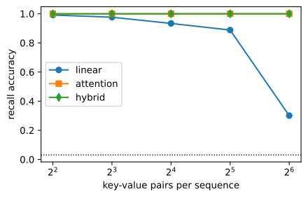
d2l.set_figsize((5, 3))
for name, marker in zip(LAYOUTS, ['o', 's', 'd']):
    d2l.plt.semilogx(loads, recall[name], marker=marker, label=name, base=2)
d2l.plt.axhline(1 / 32, color='black', lw=1, ls=':')
d2l.plt.xlabel('key-value pairs per sequence')
d2l.plt.ylabel('recall accuracy')
d2l.plt.legend();
assert min(recall['attention']) > 0.95 and min(recall['hybrid']) > 0.85
assert recall['hybrid'][-1] > 0.95 > recall['linear'][-1]  # One layer rescues
assert recall['linear'][-1] < 0.6      # The fixed state has saturated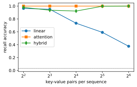
The three curves isolate the effect of one attention layer. The pure linear-recurrence stack degrades as the load grows; at 64 pairs, where it recovers fewer than half of the queries — consistent with the crowding heuristic’s cliff for \(8 \times 8\) states asked to hold 64 bindings, though read that as a diagnostic analogy: the proposition’s random-key assumptions do not cover this trained, four-layer model. The pure attention stack scores 1.000 at every load in both frameworks’ runs: its “state” at the query is the whole write phase, so load never crowds it. And the hybrid tracks attention closely, though three quarters of it is the same recurrence that just collapsed — in our PyTorch run it too scores 1.000 at every load; in JAX it dips to roughly 0.92–0.94 mid-sweep and returns to 0.99–1.00 at the two largest loads, exactly the loads that break the linear stack. One mid-stack attention layer recovers the recall deficit in this diagnostic. Controlled studies at the hundred-million-parameter scale report that adding attention to a Mamba backbone lifts recall benchmarks by about thirty points while moving reasoning benchmarks by single digits (Lee et al. 2025).
12.7.3.3 The Language-Modeling Panel
Pure recurrent language models can remain competitive because average language-modeling loss is insensitive to this recall deficit. We train the same three stacks — same widths, same blocks, nothing changed but the input pipeline — as character-level language models on The Time Machine of Section 8.5, with a 128-character context so that the window is long enough for recall to matter in principle.
class CharLM(nn.Module):
    def __init__(self, layout, vocab_size, max_len, num_hiddens=32,
                 num_heads=4):
        super().__init__()
        self.emb = nn.Embedding(vocab_size, num_hiddens)
        self.pos_emb = nn.Embedding(max_len, num_hiddens)
        self.blocks = make_blocks(layout, num_hiddens, num_heads)
        self.norm = nn.LayerNorm(num_hiddens)
        self.head = nn.Linear(num_hiddens, vocab_size)

    def forward(self, X):
        pos = torch.arange(X.shape[1], device=X.device)
        H = self.emb(X) + self.pos_emb(pos)
        for blk in self.blocks:
            H = blk(H)
        return self.head(self.norm(H))

def train_lm(layout, data, lr=3e-3):
    device, vocab = d2l.try_gpu(), len(data.vocab)
    torch.manual_seed(0)
    model = CharLM(layout, vocab, data.num_steps).to(device)
    opt = torch.optim.Adam(model.parameters(), lr=lr)
    for X, y in data.train_dataloader():
        X, y = X.to(device), y.to(device)
        loss = F.cross_entropy(model(X).reshape(-1, vocab), y.reshape(-1))
        opt.zero_grad(); loss.backward(); opt.step()
    with torch.no_grad():
        total = count = 0
        for X, y in data.val_dataloader():
            X, y = X.to(device), y.to(device)
            total += float(F.cross_entropy(model(X).reshape(-1, vocab),
                                           y.reshape(-1), reduction='sum'))
            count += y.numel()
    return total / count

data = d2l.TimeMachine(batch_size=64, num_steps=128, num_train=51200,
                       num_val=4096, tokenization='char')
print(f"{'model':>10} {'val loss':>9} {'bits/char':>10}")
lm_loss = {}
for name, layout in LAYOUTS.items():
    lm_loss[name] = train_lm(layout, data)
    print(f'{name:>10} {lm_loss[name]:>9.2f} '
          f'{lm_loss[name] / math.log(2):>10.2f}')
assert max(lm_loss.values()) - min(lm_loss.values()) < 0.15
model val loss bits/char
linear 1.75 2.52
attention 1.83 2.64
hybrid 1.76 2.54class CharLM(nnx.Module):
def __init__(self, layout, vocab_size, max_len, num_hiddens=32,
num_heads=4, rngs=None):
rngs = nnx.Rngs(0) if rngs is None else rngs
self.emb = nnx.Embed(vocab_size, num_hiddens, rngs=rngs)
self.pos_emb = nnx.Embed(max_len, num_hiddens, rngs=rngs)
self.blocks = make_blocks(layout, num_hiddens, num_heads, rngs)
self.norm = nnx.LayerNorm(num_hiddens, rngs=rngs)
self.head = nnx.Linear(num_hiddens, vocab_size, rngs=rngs)
def __call__(self, X):
H = self.emb(X) + self.pos_emb(jnp.arange(X.shape[1]))
for blk in self.blocks:
H = blk(H)
return self.head(self.norm(H))
def train_lm(layout, data, lr=3e-3):
vocab = len(data.vocab)
model = CharLM(layout, vocab, data.num_steps, rngs=nnx.Rngs(0))
optimizer = nnx.Optimizer(model, optax.adam(lr), wrt=nnx.Param)
@nnx.jit
def train_step(model, optimizer, X, y):
def loss_fn(model):
return optax.softmax_cross_entropy_with_integer_labels(
model(X), y).mean()
loss, grads = nnx.value_and_grad(loss_fn)(model)
optimizer.update(model, grads)
return loss
for X, y in data.train_dataloader():
train_step(model, optimizer, jnp.asarray(X), jnp.asarray(y))
total = count = 0
for X, y in data.val_dataloader():
losses = optax.softmax_cross_entropy_with_integer_labels(
model(jnp.asarray(X)), jnp.asarray(y))
total += float(losses.sum())
count += losses.size
return total / count
data = d2l.TimeMachine(batch_size=64, num_steps=128, num_train=51200,
num_val=4096, tokenization='char')
print(f"{'model':>10} {'val loss':>9} {'bits/char':>10}")
lm_loss = {}
for name, layout in LAYOUTS.items():
lm_loss[name] = train_lm(layout, data)
print(f'{name:>10} {lm_loss[name]:>9.2f} '
f'{lm_loss[name] / math.log(2):>10.2f}')
assert max(lm_loss.values()) - min(lm_loss.values()) < 0.15 model val loss bits/char
linear 1.76 2.54
attention 1.84 2.66
hybrid 1.77 2.55All three land within roughly a tenth of a nat of one another — about a tenth of a bit per character — and in our runs the pure-linear stack matches or beats the pure-attention stack: the model that just failed on the recall sweep is, by the language-modeling objective, the equal of the models that aced it. This run uses one pass over one small corpus at one seed. It therefore demonstrates only that perplexity can remain nearly unchanged while exact recall degrades. The larger-scale evidence says the dissociation is the rule, though: across seventeen trained language models most of the efficient-architecture perplexity gap concentrated on the rare recall tokens (Arora, Eyuboglu, Timalsina, et al. 2024), and in controlled hybrid-ratio sweeps recall climbs steeply with the attention fraction while perplexity barely responds (Wang et al. 2025). The mechanism is the same at both scales: next-character prediction on ordinary text is dominated by local structure that a compressed, always-on state models well, and the tokens that require exact long-range retrieval are too rare to move the average. Perplexity was blind to the recall deficit — which is why the field needed MQAR-style probes and needle-in-a-haystack evaluations to see it at all (Arora, Eyuboglu, Timalsina, et al. 2024; Waleffe et al. 2024), and why a perplexity-matched “efficient” model can quietly fail as a retrieval engine in production. Benchmark what you actually need.
12.7.3.4 Measured Inference State
The third panel is the other side of the trade, on our own models. At generation time an attention layer must carry its keys and values for the whole context, Equation 11.3.1; a scalar-gated layer carries its \(d_k \times d_v\) state per head. As in Figure 12.7.1, we count only the persistent decode state — the bytes a server must hold for a user between decode steps. Parameters, activations, and workspace are excluded; they are nearly identical across the three stacks anyway, as the parameter counts above showed. Counting those bytes per model at our toy width (float32, batch of one):
num_heads, d_head, fp_bytes = 4, 8, 4
kv_layer = lambda T: 2 * T * num_heads * d_head * fp_bytes
state_layer = num_heads * d_head * d_head * fp_bytes

lengths = 2 ** np.arange(6, 17)
d2l.set_figsize((5, 3))
for name, layout in LAYOUTS.items():
    per_model = [sum(kv_layer(T) if c == 'A' else state_layer
                     for c in layout) / 2**10 for T in lengths]
    d2l.plt.loglog(lengths, per_model, label=name, base=2)
d2l.plt.xlabel('context length (tokens)')
d2l.plt.ylabel('persistent decode state (KiB)')
d2l.plt.legend();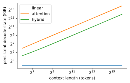
num_heads, d_head, fp_bytes = 4, 8, 4
kv_layer = lambda T: 2 * T * num_heads * d_head * fp_bytes
state_layer = num_heads * d_head * d_head * fp_bytes

lengths = 2 ** np.arange(6, 17)
d2l.set_figsize((5, 3))
for name, layout in LAYOUTS.items():
    per_model = [sum(kv_layer(T) if c == 'A' else state_layer
                     for c in layout) / 2**10 for T in lengths]
    d2l.plt.loglog(lengths, per_model, label=name, base=2)
d2l.plt.xlabel('context length (tokens)')
d2l.plt.ylabel('persistent decode state (KiB)')
d2l.plt.legend();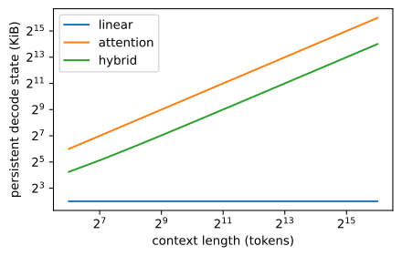
The attention stack’s line grows linearly with context; the linear stack’s is flat at four kilobytes at every length; and the hybrid’s line grows with exactly one quarter of the attention stack’s slope because one of its four layers stores keys and values per token. That slope ratio equals the attention fraction: Figure 12.7.1 is this same plot at production width, where the gap between the lines is measured in tens of gigabytes. Both sides of the trade are now on the table, from our own runs: the hybrid recalls like the attention model while using one quarter of the attention stack’s context-dependent state.
What the experiment shows: at this scale, on this diagnostic, one attention layer in four recovers pure attention’s recall while paying a quarter of its growing state — with the caveats already given (single seeded runs, a learning rate the pilot sweep pinned, a capacity heuristic rather than a theorem). What it does not show: that the result transfers to billion-parameter models trained on language. For that, the ablation studies and shipped configurations of the next two sections are the evidence.
12.7.4 Empirical Design Rules
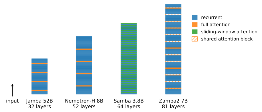
Our experiment fixed one design by fiat: one attention layer in four, mid-stack, full attention, one recurrence. Each of those choices is an axis, and by now each has been swept — by ablation studies at the hundred-million-to-billion scale, and by the engineering teams whose models the recipe table below records. Figure 12.7.2 shows the configurations of four representative systems.
How much attention? Less than you would guess, with a measurable knee. The founding ablation is NVIDIA’s 8B study (Waleffe et al. 2024): in a sweep of the attention fraction, validation loss was best near 8% attention and degraded above it — more attention is not monotonically better — yielding the recipe (roughly 43% Mamba-2, 7% attention, 50% MLP layers) that Nemotron-H and Granite ship nearly verbatim. Sequential hybrids in production cluster at 8–12.5% full attention (Jamba and MiniMax at 12.5%, Nemotron-H near 8%, Granite at 10%), with Hunyuan-TurboS lowest at 5.5% (Tencent Hunyuan Team 2025). The gated-DeltaNet family sits deliberately higher: Qwen3-Next fixes one full-attention layer per four (Qwen Team 2025), and Kimi Linear’s ablation of the ratio \(\{0{:}1, 1{:}1, 3{:}1, 7{:}1\}\) places the knee at 3:1 — at 7:1 training loss matched but validation degraded, at 1:1 quality did not improve despite the additional cost, and pure attention (0:1) was strictly worse (Kimi Team 2025). Controlled academic sweeps agree from the other side: recall climbs steeply with the attention fraction up to about 1:3 while perplexity stays nearly flat across the whole range (Wang et al. 2025) — the ratio axis is a recall dial, not a perplexity dial, which is our dissociation panel again, now as a design tool.
Where does it go? Evenly spread, and — in every report so far — not first. Waleffe et al. (2024) found no placement better than even spacing with the first layer recurrent; the systematic study of Bae et al. (2025) is blunter — “never place Transformer blocks at the front” — and finds middle placement optimal, which is why our toy hybrid put its one attention layer third of four. Samba supplies the sharpest single datapoint: inserting one full-attention layer at the front of its stack made length extrapolation collapse (perplexity exploding by 16K context), where the same capacity spent elsewhere extrapolated to 256K (Ren et al. 2024). The shipped models agree: Nemotron-H’s four attention layers sit at depths 8, 19, 30, 41 of 52 (NVIDIA 2025); Granite’s at 6, 16, 26, 36 of 40 (IBM Granite Team 2025); Jamba’s at 4, 12, 20, 28 of 32 (Lieber et al. 2024). None of these puts attention at layer one. Read the rule as a heuristic distilled from a handful of systematic studies plus shipped practice — consistent so far, but extracted from a young design space, not derived from anything.
Sequential or parallel? Interleaving whole layers is not the only composition. Hymba runs attention heads and Mamba-2 heads in parallel inside every layer, on the same input, outputs normalized and fused — and its controlled ablation has the parallel form beating the equivalent sequential stack (45.2% against 44.1% average on its commonsense suite), the argument being that the two mixers see the same representation rather than each other’s output (Dong et al. 2024). Falcon-H1 makes the same bet with a continuously tunable split of channels between the attention and SSM branches (Zuo et al. 2025), and the systematic comparison of Bae et al. (2025) places intra-layer hybrids on the best quality-efficiency Pareto frontier, slightly ahead of inter-layer. Sequential remains the production default — it is simpler to schedule and to distill into — but the parallel results say the margin is real, not folklore.
Sharing the attention you keep. Zyphra’s Zamba pushes the economics one step further: a single attention block whose weights are shared, re-entered every six Mamba layers (thirteen times in the 7B model), so global attention costs one block of parameters; Zamba2 refines this to two shared blocks applied alternately, each re-entry specialized by a cheap LoRA adapter (Glorioso, Anthony, Tokpanov, Whittington, et al. 2024; Glorioso, Anthony, Tokpanov, Golubeva, et al. 2024). Parameter sharing is orthogonal to the sequential-parallel axis, and it sharpens the section’s moral: if a few attention layers carry retrieval, perhaps they do not even need to be different layers.
Interaction between components. The components of a hybrid are not chosen independently, and the cleanest evidence is a negative result. AI21 tested Mamba-2 — larger state, better standalone model — inside Jamba and rejected it: the Mamba-1-plus-attention combination trained better, their hypothesis being that once full-attention layers can pool the entire context, the recurrence no longer needs the larger state that made Mamba-2 win in isolation (Lieber et al. 2024). The same report found no substantial quality difference between 1:3 and 1:7 attention ratios at their scale, so they shipped the cheaper. Both decisions generalize: a hybrid’s recurrent half should be judged in the presence of its attention half, and where quality saturates, economics decides. Sliding-window attention re-enters here as a middle option — Samba’s alternation of Mamba with windowed attention contains no global layer at all, yet recovers most of the recall gap and extrapolates to 256K, because a little local exact attention is already most of what retrieval needs (Ren et al. 2024), the production echo of Based’s finding that a small sliding window plus a linear global memory recovers over 90% of full attention’s recall (Arora, Eyuboglu, Zhang, et al. 2024).
12.7.5 The Recipe Table
As in Section 11.7, we close the survey with the shipped configurations themselves — one row per production hybrid, verified against each model’s technical report or released configuration. The convergence is looser than the transformer recipe’s (this design space is younger), but the clustering is already unmistakable: a strong recurrence from the ladder of Table 12.5.1, roughly a tenth to a quarter of layers as attention, evenly spread and none first, with the attention layers wearing the cache compressions of Section 11.3.
| model | layers | attention: count, positions | attention variant | recurrence | context |
|---|---|---|---|---|---|
| Jamba (52B-A12B) (Lieber et al. 2024) | 32 | 4 (12.5%), at 4/12/20/28 | full, GQA \(32{:}8\) | Mamba-1 | 256K |
| Samba (3.8B) (Ren et al. 2024) | 64 | none full; SWA every 2nd layer | SWA 2048, near-MQA | Mamba-1 | 4K train, 256K recall |
| Zamba2 (7B) (Glorioso, Anthony, Tokpanov, Golubeva, et al. 2024) | 81 | 13 re-entries of 2 shared blocks | full MHA \(32{:}32\), LoRA per call | Mamba-2 | 4K |
| Nemotron-H (8B) (NVIDIA 2025) | 52 | 4 (7.7%), at 8/19/30/41 | full, GQA \(32{:}8\) | Mamba-2 | 8K |
| Granite 4.0-H (32B-A9B) (IBM Granite Team 2025) | 40 | 4 (10%), at 6/16/26/36 | full, GQA \(32{:}8\), NoPE | Mamba-2 | 128K |
| MiniMax-01 (456B-A46B) (MiniMax 2025) | 80 | 10 (12.5%), every 8th | full, GQA \(64{:}8\) | lightning attention | 1M |
| Qwen3-Next (80B-A3B) (Qwen Team 2025) | 48 | 12 (25%), every 4th | gated attn, GQA \(16{:}2\) | gated DeltaNet | 262K |
| Kimi Linear (48B-A3B) (Kimi Team 2025) | 27 | 7 (26%), 3 KDA per MLA | MLA, NoPE | KDA (gated DeltaNet) | 1M |
| Falcon-H1 (34B) (Zuo et al. 2025) | — | parallel: attn \(\parallel\) SSM channels, every layer | full, GQA | Mamba-2 | 256K |
The columns connect these architectural choices to deployed systems. The recurrence column is the family developed in the preceding three sections— Mamba-1/2 from Section 12.3, gated DeltaNet and its per-channel refinement KDA from Section 12.5.4 (the cell we trained on our scoreboard is the one Qwen3-Next ships). The attention-variant column shows the composition argument in action: Kimi Linear pairs its recurrence with MLA, Granite and Kimi drop positional encodings on the attention layers (NoPE), Qwen3-Next keeps only 2 key–value heads — the surviving cache accounts for most of the memory, so it receives every compression Section 11.3 taught. And the context column explains the investment: the models built for the longest contexts are hybrids of this table’s shape, because Equation 11.3.1 made the alternative more expensive in hardware.
12.7.6 Distillation from Pretrained Transformers
One practical question remains: must a hybrid be pretrained from scratch? No — a pretrained transformer can be converted, and the state-space duality explains why conversion has a head start without guaranteeing it. The duality of Section 12.4.2 is an exact statement about linear attention: a semiseparable mixing matrix can be computed as a recurrence or as a masked matmul. A pretrained transformer’s softmax attention is not in that family, so its weights are not a recurrence in disguise — but its projections and per-layer mixing patterns are close enough to serve as a warm start: initialize the student’s recurrence from the attention projections and learn the rest. MOHAWK distills in three stages — match each layer’s mixing matrix (the attention pattern against the recurrence’s semiseparable approximation of it), then match hidden states, then fine-tune end to end — and turns Phi-1.5 into a Mamba-architecture model using about 3B tokens, under one percent of a from-scratch pretraining budget, with quality above same-size from-scratch Mamba models (Bick et al. 2024). “The Mamba in the Llama” initializes the recurrence directly from the attention projections and converts Llama-3 into a hybrid, keeping a fraction of attention layers intact; quality falls smoothly as attention is removed, the shipped configuration keeps about a quarter, and the distilled hybrid still solves needle-in-a-haystack at twenty times its training length — while the zero-attention variant does not (Wang et al. 2024). Both are learned approximations, not exact conversions: the duality supplies the initialization and the layer-wise matching targets, and the distillation data supplies whatever softmax attention computed that a linear recurrence cannot. The retained attention layers are where the recall lives, which by this point in the section is not a surprise; it is the design rule, observed a third way.
12.7.6.1 Architecture Comparison
The chapter’s architectures differ in what they compute; what they charge lines up in one table. Each row prices one layer of one architecture on the axes this section has been trading against each other: work and persistent state when decoding token \(t\), work and sequential depth when training on a length-\(T\) sequence, and whether the training-time parallel form computes the same function as the step-by-step form in real arithmetic (floating-point reassociation still changes rounding, which Section 12.4.2 measured). Every “constant cost”, “linear time”, or “same computation” claim made along the way resolves to a cell here, and each row cites the section that established it.
| architecture | decode work per token | persistent decode state | training work | sequential depth | parallel form exact? |
|---|---|---|---|---|---|
| LSTM / GRU (Section 12.1) | \(O(d^2)\) | \(O(d)\): \(\mathbf{h}_t\) (and \(\mathbf{c}_t\)) | \(O(T d^2)\) | \(T\) | none: nonlinearity inside the recurrence (minGRU removes it, Section 12.2.1) |
| diagonal SSM, S4D (Section 12.2.5) | \(O(d N)\) | \(d N\) numbers | \(O(T d N)\) work-efficient scan, or \(O(T \log T\, d)\) FFT convolution (Section 12.2.3.2) | \(O(\log T)\) (Section 12.2.2) | yes |
| Mamba-1 (Section 12.3.2) | \(O(d N)\) | \(d_\textrm{inner} N\) numbers | \(O(T d N)\) work-efficient scan | \(O(\log T)\) | yes: selective steps are still affine |
| SSD / Mamba-2 (Section 12.4.2) | \(O(h\, d_k d_v)\) | \(h\, d_k d_v\) numbers | \(O(T C d)\) chunked matmuls (Section 12.4.3) | \(T/C\) | yes, verified to float rounding |
| GLA (Section 12.4.1.2) | \(O(h\, d_k d_v)\) | \(h\, d_k d_v\) numbers | \(O(T C d)\) chunked | \(T/C\) | yes |
| DeltaNet (Section 12.5.3) | \(O(h\, d_k d_v)\) | \(h\, d_k d_v\) numbers | \(O(T C d)\) chunked WY | \(T/C\) | yes: the WY form is exact algebra |
| softmax attention (Section 11.2, Section 11.3) | \(O(t\, d)\) — grows | \(2 t d\) numbers — grows (Equation 11.3.1) | \(O(T^2 d)\) | \(O(1)\) | trivially: the parallel form is the definition |
| 1-in-4 hybrid (this section) | \(\tfrac{3}{4} O(h\, d_k d_v) + \tfrac{1}{4} O(t\, d)\) | constant \(+\ \tfrac14\) of the cache | mixed | per component | per component |
The attention and SSD rows summarize the central tradeoff: attention pays \(t\)-dependent work and state for exact recall; the matrix-state family pays a constant for a bounded memory; the hybrid row is a convex combination with the attention fraction as the mixing weight. The exactness column records a second distinction: every linear-recurrence training method — scan, chunk, dual, WY — is a reassociation of the same arithmetic, not an approximation, which is what made their speed free of modeling cost.
So: where does this leave the fixed state? This chapter gave it five upgrades, and this section drew its boundary. The counting bound and the width-32 experiment delimit the fixed state’s exact-recall capability. Its persistent state remains constant in context length, whereas an attention cache grows with every retained token. Production stopped treating those as competing claims and shipped both, in proportions this section measured from three independent directions — ablation sweeps, shipped configurations, and distillation experiments, all pointing at a small attention minority carrying retrieval through a less expensive recurrent majority. This section did not cover the systems techniques that make the recurrent majority fast in practice — the chunked forms of Section 12.4.3 living as fused kernels, which belongs to Chapter 13; and the pretraining and post-training of full-scale language models, hybrid or not, together with the serving stacks that exploit their nearly constant persistent memory, which are the subject of the Language Models part. The pendulum question from this chapter’s introduction — whether attention remains on top on January 1, 2027 — stays open. But notice what would settle it: not a better gate or a cleverer write rule, both of which this chapter taught, but whether a learned, compressed memory can be trusted with retrieval. That is the measured question, and you now own every tool it is measured with.
12.7.7 Summary
A fixed-size state cannot perform unbounded exact recall: reproducing \(k\) tokens from a vocabulary of \(V\) requires \(k \log_2 V\) bits in the state, and a finite-state model’s error on copying uniformly random length-\(L\) strings is at least \(1 - |\mathcal{S}|/D^L\); the failure is measurable as fuzzy recall on phone-book and needle tasks long before it shows in perplexity. The economics run the other way: by Equation 11.3.1 only attention layers pay a context-proportional cache, so a hybrid’s persistent decode state is the attention fraction times the transformer’s — Jamba’s measured 4 GB against Mixtral’s 32 GB at 256K. Our three matched stacks (parameter counts printed, spread under one percent) made both claims concrete: the pure scalar-gated stack’s recall collapsed once the load crossed roughly its \(8 \times 8\)-per-head state size, one mid-stack attention layer restored recall at the loads that broke it (1.000 throughout in our PyTorch run; 0.99–1.00 at the post-collapse loads in JAX, with a mid-sweep dip to roughly 0.92–0.94), language-modeling loss barely separated the three stacks (the pure-linear model matched or beat pure attention in our runs), and the persistent decode state grew with slope equal to the attention fraction. The shipped design rules: attention fractions cluster at 5–25%, with a measured knee near 1:3 for the DeltaNet family and near 8% for Mamba-2 hybrids; placement is even and, in every report so far, not front; parallel fusion and weight sharing are live refinements; and the components interact (Jamba chose Mamba-1 because attention was present). Pretrained transformers distill into hybrids for under a percent of the original token budget — a learned approximation the duality warm-starts, with the retained attention layers carrying recall. Table 12.7.2 collects the per-layer cost and state contracts of every architecture in the chapter. Three implementation lessons from the experiment: initialize decay gates to retain, mask in log space before exponentiating a decay kernel, and normalize the memory read-out before it joins the residual stream.
12.7.8 Exercises
Copy bound. The copy bounds of Section 12.7.1 state that a model that passes its input through a finite state set \(\mathcal{S}\) errs with probability at least \(1 - |\mathcal{S}|/D^L\) when it copies a string drawn uniformly from the \(D^L\) strings of length \(L\).
- Prove the bound for a model whose output after reading the string is a deterministic function of its state. Then show that the bound still holds when the model samples its output from a distribution that depends only on the state.
- Show that a stack of recurrent layers and sliding-window attention layers with window \(w\), without any global attention layer, is a finite-state model at fixed precision, so that the bound applies to it. After fine-tuning at 4K tokens, Samba, a stack of this kind, retrieves a 5-digit passkey hidden at any depth of a 256K-token document almost perfectly (Ren et al. 2024). Explain why this result does not contradict the bound.
Repeated n-grams. The transformer half of the copy bounds in Section 12.7.1 finds each next token by locating the earlier occurrence of the \(n\) most recently emitted tokens and reading the token that follows it. The construction is therefore guaranteed to copy correctly whenever no substring of length \(n\) occurs twice in the input. Let the input be drawn uniformly from the strings of length \(L\) over an alphabet of size \(D\).
- Show that the substrings of length \(n\) that start at two distinct positions are equal with probability exactly \(D^{-n}\), also when they overlap.
- Deduce the expected number of pairs of positions whose substrings of length \(n\) are equal, and explain why it bounds the probability that the construction fails. For \(D = 32\), find the smallest \(n\) that makes this expectation smaller than \(0.01\) at \(L = 10^3\) and at \(L = 10^4\).
- Show that \(n \ge 2 \log_D L + \log_D \frac{1}{2\delta}\) keeps the expectation of the previous part below \(\delta\) for every \(L\), and check this against the two values of \(n\) found there for \(\delta = 0.01\). How does the width \(O(n \log D)\) of the transformer then grow with \(L\) at fixed \(\delta\), and how does this compare with the number of bits that a fixed state needs in order to copy the same strings?
Million-token decode state. Consider 48-layer models that serve a context of \(2^{20}\) tokens to a batch of one in 16-bit precision. In Equation 11.3.1, every attention layer has \(n_\textrm{kv} = 8\) key–value heads of dimension \(d_\textrm{head} = 128\). Every recurrent layer holds the Mamba-2 state of Section 12.7.2, \(8192 \cdot 128\) numbers per Equation 12.4.7, and the convolution buffer is neglected.
- Find the context length at which the cache of one attention layer equals the state of one recurrent layer.
- Compute the persistent decode state of a pure transformer, of a pure recurrent stack, and of a hybrid with 6 attention layers. How many concurrent users fit into 80 GiB of free accelerator memory under each design? Check the method against Jamba, which has 4 attention layers of this shape and reports a 4 GB cache at 256K tokens (Lieber et al. 2024).
- Find the largest number of attention layers that still lets 8 users share the 80 GiB at this context, and compare the resulting attention fraction with the fractions in Table 12.7.1.
- For each of the following changes to the hybrid, state whether it changes the slope of the persistent decode state as a function of context length, its constant part, or neither: halving \(n_\textrm{kv}\); storing the cache in 8 bits; restricting every attention layer to a window of 2048 tokens; storing the recurrent states in 8 bits; and replacing the 6 attention layers by one attention block whose weights are shared across the 6 depths, as in Zamba.
[code] Gate initialization.
ScalarGatedMixerinitializes the bias ofW_gat \(-4.5\). Neglect the input-dependent part of the gate, so that a bias \(b\) gives the decay \(a = \exp(-\textrm{softplus}(b))\).- For \(b \in \{0, -2, -4.5, -8\}\), compute \(a\), the half-life of the state in tokens, and the weight \(a^{2P-1}\) with which the first binding of a sequence from
make_recallreaches the last query of that sequence, atnum_pairs\(P \in \{8, 64\}\). - Give
ScalarGatedMixera constructor argument for the bias, pass it throughmake_blocks,RecallModel, andtrain_recall, and train'GGGG'and'GGAG'atnum_pairs\(\in \{8, 32\}\) for each \(b\). Predict before training which of the two layouts depends on \(b\). Explain the results from the first part and from what the attention layer reads.
- For \(b \in \{0, -2, -4.5, -8\}\), compute \(a\), the half-life of the state in tokens, and the weight \(a^{2P-1}\) with which the first binding of a sequence from
Overflow in the dual.
ScalarGatedMixerforms \(\textrm{logL}_{ij} = \textrm{cum}_i - \textrm{cum}_j\) with \(\textrm{cum}_t = \sum_{r \le t} \log a_r\), replaces the entries above the diagonal by \(-\infty\), and then exponentiates. Suppose that it exponentiated first and multiplied by the causal mask afterwards.- Find the largest entry of \(\exp(\textrm{logL})\) above the diagonal for a sequence of length \(T\), in terms of the decays. For a constant decay \(a\), find the values of \(a\) for which this entry overflows float32, whose largest finite value is about \(3.4 \times 10^{38}\), at \(T = 128\). Compare these values with the decays \(a = \exp(-\textrm{softplus}(b))\) for the biases \(b = 0\) and \(b = -4.5\), which neglect the input-dependent part of the gate. Then use the convexity of softplus to decide in which direction the input-dependent part moves the case \(b = 0\), and explain why a head trained only on the recall task is unlikely to overflow.
- Replace the multiplication by a selection that returns \(0\) above the diagonal and \(\exp(\textrm{logL})\) on and below it. For a decay at which the entry of the first part overflows, show that the forward pass is now finite but that the gradient with respect to the decays is not. Explain why replacing the entries by \(-\infty\) before the exponential gives finite gradients.
Read-out scale. Before its RMSNorm,
ScalarGatedMixerreads out\[\mathbf{o}_t = \sum_{s \le t} a^{t-s}\, \frac{\mathbf{q}_t^\top \mathbf{k}_s}{\sqrt{d_\textrm{head}}}\, \mathbf{v}_s, \tag{12.7.1}\]
where this problem takes the decay \(a\) to be constant. Let all entries of the queries, keys, and values be independent with mean zero and variance one.
- Show that every coordinate of \(\mathbf{o}_t\) has variance \((1 - a^{2t})/(1 - a^2)\), read as \(t\) when \(a = 1\), and evaluate it at \(t = 128\) for \(a = 0.5\), \(a = 0.989\), and \(a = 1\).
- Softmax attention reads out \(\mathbf{o}_t = \sum_{s \le t} p_{ts} \mathbf{v}_s\) with weights \(p_{ts} \ge 0\) that sum to one and are independent of the values. Bound the variance of each coordinate of its read-out. Use both results to explain why the attention mixer needs no read-out normalization, and how the gate initialization of Section 12.7.3.1 changes the need for it in the scalar-gated mixer.
Capacity accounts. The decode state of the stack
'GGGG'consists of 4 layers with 4 heads each, and every head holds an \(8 \times 8\) matrix. The recall task of Section 12.7.3 draws its keys from 64 ids and its values from 32.- Count the bits of this state in float32 and the bits that an answer to every query requires at
num_pairs=64. Repeat the count at production scale for a stack of 48 recurrent layers, each holding the Mamba-2 state of Section 12.7.2 (\(8192 \cdot 128\) numbers in fp16), with a vocabulary of \(2^{17}\) tokens: find the smallest length \(L\) at which the copy bound of Section 12.7.1 forces an error of at least \(1/2\). Does the bound explain the collapse of'GGGG'at 64 pairs, or the phone-book failures of the pure Mamba-2 model in Section 12.7.1? - Suppose that each head stores its bindings under mutually orthogonal keys. How many bindings can one head hold without interference, how many can one layer hold, and how many can the stack hold if every layer stores different keys?
- Under independent random unit keys, the crowding proposition Equation 12.4.3 makes the expected read error of a head equal to its unit signal at some load. Find that load and the load of one layer whose heads split the bindings evenly. Compare the three accounts with the accuracies of
'GGGG'in Section 12.7.3.2. What does the comparison suggest about the keys that training finds?
- Count the bits of this state in float32 and the bits that an answer to every query requires at
[code] A window instead. ● Samba replaces global attention by sliding-window attention (Ren et al. 2024). Test this choice on the recall task with a window of 16 positions, in which each query attends to itself and to the 15 positions before it.
- Write
WindowAttention, a subclass ofd2l.GPT.CausalAttentionthat masks the scores outside the window before the softmax. Check on a random input that the output at position \(t\) changes when the input at position \(t - 15\) changes, and that it does not change when the input at position \(t - 16\) or at any position after \(t\) changes. - Call a query of a sequence from
make_recallcovered if the write of its key lies inside its window. Compute the expected fraction of covered queries as a function ofnum_pairs, and find the largestnum_pairsat which every query is covered. - Add a letter
'W'for the new mixer tomake_blocks, and run the recall sweep for'GGWG'. Compare its accuracy at each load with the covered fraction and with the accuracies of'GGGG'and'GGAG'. What do the recurrent layers contribute, and what does the result suggest about hybrids without a global attention layer?
- Write
[code] Recall slice. ● Arora, Eyuboglu, Timalsina, et al. (2024) found most of the perplexity gap between efficient models and attention on the tokens that require recall. Call a target character of a validation window a repeat if the 8 characters ending at it, the target and its 7 predecessors, also occur in this order earlier in the same window.
- Modify
train_lmto also return the trained model. For each of the three stacks of Section 12.7.3.3, compute the mean validation loss on the repeat targets and on all other targets. - Measure the fraction of repeat targets. Suppose that a model predicted every repeat target at chance and every other target as well as the best stack. Bound the resulting increase of its average loss, and compare the bound with the spread of 0.15 nats that the assertion of Section 12.7.3.3 allows.
- Does the repeat slice separate the three stacks where the average loss does not? Explain the result from what each mixer can retrieve from a context of 128 characters.
- Modify
Softmax block rank. ● Split a sequence of length \(T\) after position \(\tau\). For a causal mixer \(\mathbf{Y} = \mathbf{M}\mathbf{V}\), the block \(\mathbf{M}_{>\tau, \le \tau}\) carries everything that the outputs after \(\tau\) take from the values up to \(\tau\). For the scalar-gated mixer, \(\mathbf{M} = \mathbf{L} \circ \mathbf{Q}\mathbf{K}^\top\) of Equation 12.4.6, and this block has rank at most \(d_k\), because the later outputs see the earlier values only through the state. Softmax attention has
\[M_{ts} = \frac{\exp(\mathbf{q}_t^\top \mathbf{k}_s / \sqrt{d_k})}{\sum_{r \le t} \exp(\mathbf{q}_t^\top \mathbf{k}_r / \sqrt{d_k})} \quad \textrm{for } s \le t. \tag{12.7.2}\]
- Let \(d_k = 1\), \(q_t = t\), and \(k_s = s\), and drop the factor \(1/\sqrt{d_k}\). Show that the block of the softmax mixing matrix has rank \(\min(\tau, T - \tau)\). Conclude that no recurrence whose fixed-size state is linear in the values reproduces a softmax head exactly at every sequence length.
- Expand the exponential in its power series. Show that the term of degree \(p\) contributes a block of rank at most \(\binom{d_k + p - 1}{p}\), and that truncating the series after degree \(p\) gives a linear attention whose feature map has \(\sum_{j \le p} \binom{d_k + j - 1}{j}\) coordinates.
- Draw \(\mathbf{q}_t, \mathbf{k}_s \in \mathbb{R}^8\) with independent \(\mathcal{N}(0, \sigma^2)\) entries, take \(T = 256\) and \(\tau = 128\), and count the singular values of the softmax block that exceed \(10^{-2}\) and \(10^{-4}\) times the largest one, for \(\sigma = 0.25\) and \(\sigma = 1\). Compare the counts with the second part and with \(d_k = 8\). Which attention heads of a pretrained transformer should a distillation into a hybrid, as in Section 12.7.6, keep as attention, and why?
[extended] Placement and length. ● The hybrid
'GGAG'puts its attention layer third of four, following the placement rules of- Run the recall sweep for
'AGGG'and'GGGA'. Explain the result from what an attention layer needs in order to look up a binding. train_recallbuildsRecallModelwith a learned position table ofmax_len = 2 * num_pairsentries, so its models cannot run on longer sequences. Modifytrain_recallto build the models withpos=Falseand to return them. Check atnum_pairs=32that'GGGG','AGGG','GGAG','GGGA', and'AAAA'reach the accuracies they reach with positions.- Extend
make_recallto insert \(m\) filler tokens between the write phase and the query phase. Give each filler the key id 64, which no binding uses, the value id that queries carry, and the target \(-1\), and build the models withnum_keys=65. Train every layout of the second part atnum_pairs=32and \(m = 0\), and evaluate it at \(m \in \{8, 32, 128\}\). Which layouts degrade, and how do the decays and the position of the attention layer explain the differences? Does the outcome support the rule that attention should not come first?
- Run the recall sweep for