import numpy as np
import torch29.2 Neural ODEs, Adjoints, and Continuous Flows
The previous section ended with two observations about methods we have used for many chapters: a residual block is one forward-Euler step of size \(h=1\), and gradient descent is Euler’s method applied to “move downhill”. That section also showed that the exact flow of a Lipschitz field can be run backward, so it never maps two points to one. If a residual network is a numerical solution of a differential equation, what do we gain by taking the equation itself as the model, and what does it cost?
Generative modelling gives one answer. A normalizing flow is a network that can be inverted, so that every output comes from exactly one input. The density of its outputs then follows from the change-of-variables formula, which asks for the determinant of the network’s Jacobian at every sample. For a small colour image of \(32\times32\) pixels that Jacobian has \(3072\) rows, and its determinant costs about \(2\times10^{10}\) operations, thousands of times the cost of evaluating one layer on the same image. Discrete flows avoid this cost by restricting the form of their layers. A flow in continuous time avoids it differently: the determinant turns into a trace, and the trace can be estimated with one backward pass.
The model is a differential equation \(\dot{\mathbf{x}}=\mathbf{f}_{\boldsymbol\theta}(\mathbf{x},t)\) whose solution at a final time is the output, a Neural ODE (Chen et al. 2018). Training it and computing its density each come down to integrating one more equation alongside the state. For training, that equation is the adjoint equation, which optimal control developed in the 1950s to ask how the cost of a trajectory changes with its controls (Pontryagin et al. 1962). For the density, it is an integral of the trace of the Jacobian, and a model that computes it is a continuous normalizing flow (Grathwohl et al. 2019). Compared with a fixed residual stack, the model gains an invertible map, a computable density, and a step count that can be chosen after training. The diffusion samplers later in this chapter rely on the last of these when they integrate a learned field.
We train such a model through a solver, derive the adjoint and compare it with backpropagation, and then follow a density along a flow. Everything stays deterministic until the next section adds noise. Notation: the field \(\mathbf{f}_{\boldsymbol\theta}\) has parameters \(\boldsymbol\theta\) and Jacobian \(\mathbf J=\partial\mathbf{f}/\partial\mathbf{x}\), \(\Phi_t\) is its flow map, a solver takes \(N\) steps of size \(h\) to the horizon \(T=Nh\), \(\mathcal{L}\) is a loss, \(\mathbf{a}(t)\) the adjoint and \(p_t\) the density.
import numpy as np
import tensorflow as tf
import jax
from jax import numpy as jnp
import numpy as np
import optaxfrom mxnet import autograd, gluon, init, np as mnp, npx
from mxnet.gluon import nn
import numpy as np
npx.set_np()The adjoint and density checks reuse the spiral field \(\mathbf A\) and the starting point \(\mathbf{x}_0\) of Section 29.1, together with two tools from there: the matrix exponential \(e^{\mathbf Bs}=\mathbf Ve^{\boldsymbol\Lambda s}\mathbf V^{-1}\) from the eigendecomposition \(\mathbf B=\mathbf V\boldsymbol\Lambda \mathbf V^{-1}\), and the classical fourth-order Runge–Kutta solver (RK4).
A = np.array([[-0.5, -1.0], [1.0, -0.5]])      # spiral sink: eigenvalues -0.5 +- i
x0 = np.array([2.0, 0.0])

def expm_eig(B, s):
    """e^{Bs} via the eigendecomposition B = V diag(mu) V^{-1}."""
    mu, V = np.linalg.eig(B)
    return (V @ np.diag(np.exp(mu * s)) @ np.linalg.inv(V)).real

def rk4(f, x, T, n):
    """n classical RK4 steps of dx/dt = f(x) from time 0 to time T."""
    h = T / n
    for _ in range(n):
        k1 = f(x)
        k2 = f(x + h / 2 * k1)
        k3 = f(x + h / 2 * k2)
        k4 = f(x + h * k3)
        x = x + h / 6 * (k1 + 2 * k2 + 2 * k3 + k4)
    return x
29.2.1 Neural ODEs
A Neural ODE is what a residual network becomes when its depth turns into time. We first make that limit precise, then show one thing the limit cannot do, and then train a small model through its solver.
29.2.1.1 From Residual Blocks to a Continuous Model
We start from the network we already have, a stack of residual blocks, and ask which continuous model it approximates. A residual block (He et al. 2016) and a forward-Euler step of the ODE \(\dot{\mathbf{x}}=\mathbf{f}(\mathbf{x},t)\) read
\[ \mathbf{x}_{l+1}=\mathbf{x}_l+\mathbf{f}_{\boldsymbol\theta_l}(\mathbf{x}_l) \qquad\textrm{and}\qquad \mathbf{x}_{n+1}=\mathbf{x}_n+h\,\mathbf{f}(\mathbf{x}_n,t_n). \tag{29.2.1}\]
With \(h=1\) and \(\mathbf{f}(\cdot,t_l)=\mathbf{f}_{\boldsymbol\theta_l}\) the two updates are the same formula. A ResNet whose blocks have different weights is therefore a time-dependent field sampled at the layer times and integrated by Euler’s method with unit steps (Figure 29.2.1).

Why pass to the limit at all? The exact flow of an ODE has three properties that a finite stack is not guaranteed to have. It is invertible. Its effect on probability densities can be written down, as the last part of this section shows. And the number of steps used to compute it is no longer part of the model, so it can be chosen at evaluation time.
To take the limit, share one field across all steps and let the steps shrink: \(N\) steps of size \(h=T/N\) at the times \(t_n=nh\),
\[ \mathbf{x}_{n+1}=\mathbf{x}_n+h\,\mathbf{f}_{\boldsymbol\theta}(\mathbf{x}_n,t_n), \qquad \mathbf{x}_N\;\xrightarrow{\;N\to\infty\;}\; \mathbf{x}(T)=\mathbf{x}_0+\int_0^T\mathbf{f}_{\boldsymbol\theta}(\mathbf{x}(t),t)\,dt . \tag{29.2.2}\]
The convergence follows from Euler’s global error bound in Section 29.1.3: for a smooth field that is Lipschitz in \(\mathbf{x}\), the Euler iterate after \(N\) steps is within \(O(h)\) of the exact solution. The Neural ODE is the limit object: the model whose output is the solution \(\mathbf{x}(T)\) of \(\dot{\mathbf{x}}=\mathbf{f}_{\boldsymbol\theta}(\mathbf{x},t)\) with \(\mathbf{x}(0)=\mathbf{x}_0\). The parameters define the field. The solver (Euler, RK4, an adaptive method) is a choice made afterwards, which changes the computed map, its cost and its error, but not the model.
The exact map and the computed map can differ in kind, not only in accuracy. The field \(\dot{x}=-x\) has the exact flow \(\Phi_t(x)=e^{-t}x\), a bijection of \(\mathbb{R}\) for every \(t\). One Euler step with \(h=1\) computes \(x+1\cdot(-x)=0\) and maps every input to zero. The exact map, by contrast, is always invertible when the field is continuous in \(t\) and globally Lipschitz in \(\mathbf{x}\) (Section 29.1.1.4). The reversed path \(\mathbf{y}(s)=\mathbf{x}(T-s)\) solves \(\dot{\mathbf{y}}=-\mathbf{f}(\mathbf{y},T-s)\), whose field is again Lipschitz. So every endpoint is reached from exactly one start, and running the reversed field recovers it.
29.2.1.2 Order Preservation on the Line
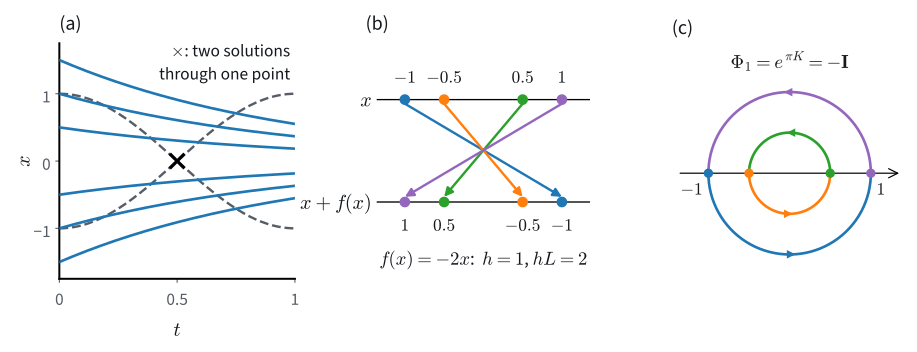
Invertibility is a gain, but it is also a constraint. Is a Neural ODE at least as expressive as the residual stack it came from? On the real line it is not, and a picture shows why. In the \((t,x)\) plane, trajectories of a Lipschitz field never cross. Two trajectories that swapped \(-1\) and \(1\) would have to meet on the way (panel (a) of Figure 29.2.2).
Proposition (flows on \(\mathbb{R}\) preserve order). Let \(f(x,t)\) be continuous in \(t\) and globally Lipschitz in \(x\), and write \(\Phi_t(x)\) for the solution at time \(t\) started from \(x\) at time \(0\). Then for every \(T>0\) the map \(\Phi_T\) is strictly increasing.
Proof. Let \(x<y\) and suppose \(\Phi_T(x)\ge\Phi_T(y)\). The function \(g(t)=\Phi_t(y)-\Phi_t(x)\) is continuous with \(g(0)>0\) and \(g(T)\le0\), so by the intermediate value theorem \(g(s)=0\) for some \(s\in(0,T]\): the two trajectories meet at time \(s\) at a point \(z\). Now run time backward from \(s\). Both reversed trajectories \(\tau\mapsto\Phi_{s-\tau}(x)\) and \(\tau\mapsto\Phi_{s-\tau}(y)\) solve the same initial-value problem \(\dot{w}=-f(w,s-\tau)\), \(w(0)=z\), whose field is again Lipschitz. By Picard–Lindelöf that problem has only one solution, so the two reversed trajectories coincide, and at \(\tau=s\) this says \(x=y\), a contradiction. \(\blacksquare\)
The step that is not routine is to apply uniqueness backward, from the meeting time. Thus no Neural ODE on \(\mathbb{R}\) realizes \(x\mapsto-x\): that map sends \(-1\) to \(1\) and \(1\) to \(-1\), which reverses their order.
The residual block \(x+f(x)\) with \(f(x)=-2x\) does realize it, in one step (panel (b) of Figure 29.2.2). That block is the Euler step with \(h=1\) of \(\dot{x}=-2x\), whose exact flow \(e^{-2t}x\) never reverses order. The two statements agree because one Euler step \(x+hf(x)\) of a field with Lipschitz constant \(L\) is guaranteed to be increasing when \(hL<1\): for \(x>y\),
\[ \big(x+hf(x)\big)-\big(y+hf(y)\big)\;\ge\;(x-y)-hL\,(x-y)\;=\;(1-hL)(x-y), \]
which is positive when \(hL<1\). Here \(hL=2\), so the step may reverse order. A finite step is not a flow, and the proposition does not constrain it.
One more dimension removes the obstruction. Let \(\mathbf K=\left(\begin{smallmatrix}0&-1\\1&0\end{smallmatrix}\right)\), which satisfies \(\mathbf K^2=-\mathbf{I}\), so that the exponential series splits into \(e^{s\mathbf K}=\cos s\,\mathbf{I}+\sin s\,\mathbf K\), the rotation by the angle \(s\). The field \(\dot{\mathbf{x}}=\pi \mathbf K\mathbf{x}\) has the time-one map
\[ \Phi_1=e^{\pi \mathbf K}=\cos\pi\,\mathbf{I}+\sin\pi\,\mathbf K=-\mathbf{I}. \]
It carries \((x,0)\) to \((-x,0)\) along half circles, and trajectories pass each other in the plane without meeting (panel (c) of Figure 29.2.2). Adding dimensions in this way is called augmentation (Dupont et al. 2019). A flow is a continuous rearrangement of space, and on a line there is no room for two points to pass.
29.2.1.3 Training Through the Solver
The forward pass of a Neural ODE is a loop of \(N\) solver steps. The direct way to train it is to discretize, then differentiate: write the solver into the computation graph, compute the loss on \(\mathbf{x}_N\), and backpropagate through the unrolled steps. With Euler as the solver the program is a ResNet of \(N\) blocks that share one set of weights, so ordinary automatic differentiation trains it.
Can ten shared-weight residual updates learn a prescribed deformation of the plane? We take a field with one hidden layer of \(32\) tanh units and ask that its time-one flow carry \(64\) points of the unit circle to the matching points of the ellipse centred at \((1.5,0)\) with semi-axes \(1.2\) and \(0.4\). The loss is the mean squared error at the endpoints, the solver takes \(N=10\) Euler steps of size \(h=0.1\), and Adam (Section 26.4) runs \(400\) full-batch iterations at learning rate \(0.05\), lowered to \(0.005\) for the last \(100\). The function flow takes the step count and step size as arguments, so that the trained field can later be integrated in other ways.
angle = np.linspace(0, 2 * np.pi, 64, endpoint=False)
X0_ring = np.stack([np.cos(angle), np.sin(angle)], axis=1)            # circle
X1_ring = np.stack([1.5 + 1.2 * np.cos(angle), 0.4 * np.sin(angle)], axis=1)
X, Y = torch.tensor(X0_ring).float(), torch.tensor(X1_ring).float()
net = torch.nn.Sequential(torch.nn.Linear(2, 32), torch.nn.Tanh(),
                          torch.nn.Linear(32, 2))
for layer in net[::2]:                         # Glorot-uniform weights, zero biases
    torch.nn.init.xavier_uniform_(layer.weight)
    torch.nn.init.zeros_(layer.bias)

def flow(X, N=10, h=0.1, sign=1.0):
    """N Euler steps of size h; sign=-1 integrates the field backward."""
    for _ in range(N):                         # one Euler step = one residual block
        X = X + sign * h * net(X)
    return X

opt = torch.optim.Adam(net.parameters(), lr=0.05)
sched = torch.optim.lr_scheduler.MultiStepLR(opt, [300], 0.1)  # 0.005 from 300
for it in range(401):
    loss = ((flow(X) - Y) ** 2).mean()
    opt.zero_grad()
    loss.backward()
    opt.step()
    sched.step()
    if it % 200 == 0:
        print(f'iter {it:3d}  loss {loss.item():.1e}')
iter 0 loss 1.2e+00
iter 200 loss 1.3e-05
iter 400 loss 3.9e-06angle = np.linspace(0, 2 * np.pi, 64, endpoint=False)
X0_ring = np.stack([np.cos(angle), np.sin(angle)], axis=1) # circle
X1_ring = np.stack([1.5 + 1.2 * np.cos(angle), 0.4 * np.sin(angle)], axis=1)
X, Y = tf.constant(X0_ring, tf.float32), tf.constant(X1_ring, tf.float32)
net = tf.keras.Sequential([tf.keras.layers.Dense(32, activation='tanh'),
tf.keras.layers.Dense(2)]) # Glorot-uniform, zero biases
def flow(X, N=10, h=0.1, sign=1.0):
"""N Euler steps of size h; sign=-1 integrates the field backward."""
for _ in range(N): # one Euler step = one residual block
X = X + sign * h * net(X)
return X
lr = tf.keras.optimizers.schedules.PiecewiseConstantDecay([300], [0.05, 0.005])
opt = tf.keras.optimizers.Adam(learning_rate=lr) # 0.005 after iteration 300
@tf.function
def train_step():
with tf.GradientTape() as tape:
loss = tf.reduce_mean((flow(X) - Y) ** 2)
opt.apply_gradients(zip(tape.gradient(loss, net.trainable_variables),
net.trainable_variables))
return loss
for it in range(401):
loss = train_step()
if it % 200 == 0:
print(f'iter {it:3d} loss {float(loss):.1e}')iter 0 loss 1.4e+00
iter 200 loss 4.3e-06
iter 400 loss 1.1e-06angle = np.linspace(0, 2 * np.pi, 64, endpoint=False)
X0_ring = np.stack([np.cos(angle), np.sin(angle)], axis=1) # circle
X1_ring = np.stack([1.5 + 1.2 * np.cos(angle), 0.4 * np.sin(angle)], axis=1)
X, Y = jnp.array(X0_ring), jnp.array(X1_ring)
k1, k2 = jax.random.split(jax.random.key(np.random.randint(2**31)))
glorot = jax.nn.initializers.glorot_uniform() # Glorot-uniform weights, zero biases
params = {'W1': glorot(k1, (2, 32)), 'b1': jnp.zeros(32),
'W2': glorot(k2, (32, 2)), 'b2': jnp.zeros(2)}
def net(params, X):
return jnp.tanh(X @ params['W1'] + params['b1']) @ params['W2'] + params['b2']
def flow(params, X, N=10, h=0.1, sign=1.0):
"""N Euler steps of size h; sign=-1 integrates the field backward."""
step = lambda i, X: X + sign * h * net(params, X) # one residual block
return jax.lax.fori_loop(0, N, step, X)
opt = optax.adam(optax.piecewise_constant_schedule(0.05, {300: 0.1}))
opt_state = opt.init(params)
@jax.jit
def train_step(params, opt_state):
loss, grads = jax.value_and_grad(
lambda p: ((flow(p, X) - Y) ** 2).mean())(params)
updates, opt_state = opt.update(grads, opt_state)
return optax.apply_updates(params, updates), opt_state, loss
for it in range(401):
params, opt_state, loss = train_step(params, opt_state)
if it % 200 == 0:
print(f'iter {it:3d} loss {float(loss):.1e}')iter 0 loss 1.2e+00
iter 200 loss 9.1e-06
iter 400 loss 1.4e-06angle = np.linspace(0, 2 * np.pi, 64, endpoint=False)
X0_ring = np.stack([np.cos(angle), np.sin(angle)], axis=1) # circle
X1_ring = np.stack([1.5 + 1.2 * np.cos(angle), 0.4 * np.sin(angle)], axis=1)
X, Y = mnp.array(X0_ring, dtype='float32'), mnp.array(X1_ring, dtype='float32')
net = nn.HybridSequential()
net.add(nn.Dense(32, activation='tanh'), nn.Dense(2))
net.initialize(init.Xavier()) # Glorot-uniform weights, zero biases
net.hybridize()
def flow(X, N=10, h=0.1, sign=1.0):
"""N Euler steps of size h; sign=-1 integrates the field backward."""
for _ in range(N): # one Euler step = one residual block
X = X + sign * h * net(X)
return X
trainer = gluon.Trainer(net.collect_params(), 'adam', {'learning_rate': 0.05})
for it in range(401):
if it == 300:
trainer.set_learning_rate(0.005) # tenfold smaller for the last 100
with autograd.record():
loss = ((flow(X) - Y) ** 2).mean()
loss.backward()
trainer.step(1)
if it % 200 == 0:
print(f'iter {it:3d} loss {float(loss):.1e}')iter 0 loss 1.2e+00
iter 200 loss 5.6e-06
iter 400 loss 1.3e-06The loss falls from order one to well below \(10^{-4}\), typically about \(10^{-6}\): one small field, integrated by ten shared-weight residual updates, reproduces the prescribed endpoints.
Is what we trained a continuous flow or a ten-step program? Two tests answer this. First, integrate the trained field with \(N=100\) and \(N=1000\) steps (\(Nh=1\) throughout); the larger \(N\), the closer the computed map is to the exact time-one flow of the field. Second, integrate forward \(N\) steps and then backward \(N\) steps with \(\mathbf{x}\leftarrow\mathbf{x}-h\,\mathbf{f}_{\boldsymbol\theta}(\mathbf{x})\), and measure how far the round trip lands from where it started.
with torch.inference_mode():
    for n in (10, 100, 1000):
        fwd = flow(X, n, 1 / n)
        back = flow(fwd, n, 1 / n, sign=-1.0)
        err = torch.linalg.vector_norm(fwd - Y, dim=1).mean()
        trip = torch.linalg.vector_norm(back - X, dim=1).mean()
        print(f'N = {n:4d}: endpoint error {err:.1e}, '
              f'forward-backward round trip {trip:.1e}')
N = 10: endpoint error 2.5e-03, forward-backward round trip 5.6e-02
N = 100: endpoint error 1.7e-02, forward-backward round trip 5.7e-03
N = 1000: endpoint error 1.9e-02, forward-backward round trip 5.7e-04for n in (10, 100, 1000):
fwd = flow(X, n, 1 / n)
back = flow(fwd, n, 1 / n, sign=-1.0)
err = tf.reduce_mean(tf.norm(fwd - Y, axis=1))
trip = tf.reduce_mean(tf.norm(back - X, axis=1))
print(f'N = {n:4d}: endpoint error {float(err):.1e}, '
f'forward-backward round trip {float(trip):.1e}')N = 10: endpoint error 1.4e-03, forward-backward round trip 5.5e-02
N = 100: endpoint error 1.7e-02, forward-backward round trip 5.6e-03
N = 1000: endpoint error 1.9e-02, forward-backward round trip 5.6e-04for n in (10, 100, 1000):
fwd = flow(params, X, n, 1 / n)
back = flow(params, fwd, n, 1 / n, sign=-1.0)
err = jnp.linalg.norm(fwd - Y, axis=1).mean()
trip = jnp.linalg.norm(back - X, axis=1).mean()
print(f'N = {n:4d}: endpoint error {float(err):.1e}, '
f'forward-backward round trip {float(trip):.1e}')N = 10: endpoint error 1.5e-03, forward-backward round trip 5.4e-02
N = 100: endpoint error 1.7e-02, forward-backward round trip 5.5e-03
N = 1000: endpoint error 1.9e-02, forward-backward round trip 5.5e-04for n in (10, 100, 1000):
fwd = flow(X, n, 1 / n)
back = flow(fwd, n, 1 / n, sign=-1.0)
err = mnp.sqrt(((fwd - Y) ** 2).sum(axis=1)).mean()
trip = mnp.sqrt(((back - X) ** 2).sum(axis=1)).mean()
print(f'N = {n:4d}: endpoint error {float(err):.1e}, '
f'forward-backward round trip {float(trip):.1e}')N = 10: endpoint error 1.4e-03, forward-backward round trip 5.5e-02
N = 100: endpoint error 1.7e-02, forward-backward round trip 5.6e-03
N = 1000: endpoint error 1.9e-02, forward-backward round trip 5.6e-04At the training step count the endpoints lie within \(0.01\) of their targets, typically a few thousandths. With finer steps the endpoint error rises to about \(0.02\) and then stops changing. Training fitted the ten-step program. The exact time-one flow of the same field, which \(N=1000\) approximates, lands about \(0.02\) from the targets, under \(2\%\) of the ellipse’s long semi-axis. The field defines a flow close to its ten-step program, not equal to it.
The round trip misses its start by about \(0.055\) at \(N=10\), \(0.0056\) at \(N=100\) and \(0.00056\) at \(N=1000\), tenfold less per tenfold more steps. Each pair of forward and backward Euler steps leaves a residual of order \(h^2\), and \(N\) of them add up to \(O(h)\), Euler’s order. The exact flow is invertible, whereas the numerical map becomes invertible only in the limit \(h\to0\).
29.2.2 The Adjoint Method
Backpropagating through \(N\) solver steps stores the \(N\) intermediate states, and an adaptive solver does not even know \(N\) in advance. The adjoint method instead differentiates the exact flow: it integrates one linear ODE backward in time, and it can recompute the states on the way instead of storing them. Its central object is the adjoint state \(\mathbf{a}(t)=\partial\mathcal{L}/\partial\mathbf{x}(t)\), the gradient of the loss with respect to the state at time \(t\). It is the continuous analogue of the quantity that backpropagation carries from layer to layer, the gradient of the loss with respect to a layer’s output (Section 25.4).
29.2.2.1 The Scalar Case
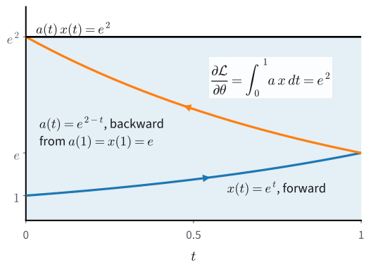
Before the general statement we work one example to the end, an example in which every quantity has a closed form. Take \(\dot{x}=\theta x\) with \(x(0)=x_0\) and the loss \(\mathcal{L}=\tfrac12x(T)^2\) on the endpoint. Directly, \(x(T)=e^{\theta T}x_0\), so \(\partial x(T)/\partial\theta=T\,x(T)\) and
\[ \frac{\partial\mathcal{L}}{\partial\theta}=x(T)\,\frac{\partial x(T)}{\partial\theta}=T\,x(T)^2 . \]
With \(\theta=T=x_0=1\) this is \(e^2=7.389\).
The adjoint reaches the same number by another route. A nudge \(\delta\) to the state at time \(t\) grows to \(e^{\theta(T-t)}\delta\) by time \(T\) and changes the loss by \(x(T)\,e^{\theta(T-t)}\delta\), so \(a(t)=e^{\theta(T-t)}x(T)\). This adjoint solves the ODE \(\dot{a}=-\theta a\) backward from the final value \(a(T)=x(T)\), which is the derivative of the loss \(\ell(x)=\tfrac12x^2\) at \(x(T)\). A change of \(\theta\) pushes the trajectory at the rate \(\partial f/\partial\theta=x\), and the adjoint converts each push into a change of the loss. Summing over time,
\[ \int_0^T a(t)\,\frac{\partial f}{\partial\theta}\,dt =\int_0^T e^{\theta(T-t)}x(T)\;e^{\theta t}x_0\,dt =\int_0^T x(T)^2\,dt =T\,x(T)^2 . \tag{29.2.3}\]
The integrand is constant: \(x\) grows forward, \(a\) shrinks by the same factor when read forward, and their product stays at \(x(T)^2\) (Figure 29.2.3). The gradient is the area under it. In words, \(a(t)\) answers “how much does the loss change if the trajectory is nudged at time \(t\)?”, and the parameter gradient adds up, over time, the nudge the parameter causes times the loss’s sensitivity to it.
29.2.2.2 The Adjoint Equations
The general case keeps the shape of the scalar one: an adjoint that runs backward from the gradient of the loss, and a parameter gradient that integrates the adjoint against \(\partial\mathbf{f}/\partial\boldsymbol\theta\).
Proposition (the adjoint equations). Let \(\mathbf{f}\) be continuously differentiable in \(\mathbf{x}\) and \(\boldsymbol\theta\), let \(\mathbf{x}(t)\) solve \(\dot{\mathbf{x}}=\mathbf{f}(\mathbf{x},\boldsymbol\theta,t)\) on \([0,T]\) from a fixed \(\mathbf{x}(0)\), and let \(\mathcal{L}=\ell(\mathbf{x}(T))\) for a differentiable \(\ell\). Then the adjoint state satisfies the linear ODE
\[ \dot{\mathbf{a}}(t) = -\left(\frac{\partial \mathbf{f}}{\partial \mathbf{x}}\right)^{\!\top}\! \mathbf{a}(t), \qquad \mathbf{a}(T) = \nabla \ell(\mathbf{x}(T)), \tag{29.2.4}\]
integrated backward from \(T\), and the parameter gradient is the integral
\[ \frac{\partial \mathcal{L}}{\partial \boldsymbol\theta} = \int_0^T \left(\frac{\partial \mathbf{f}}{\partial \boldsymbol\theta}\right)^{\!\top}\! \mathbf{a}(t)\, dt, \tag{29.2.5}\]
with both partial derivatives evaluated along the trajectory \((\mathbf{x}(t),\boldsymbol\theta,t)\) (Chen et al. 2018).
Proof (variational). Perturb the parameters by an infinitesimal \(\delta\boldsymbol\theta\). Because \(\mathbf{f}\) is \(C^1\), the solution is differentiable in \(\boldsymbol\theta\), and the first-order perturbation \(\delta\mathbf{x}(t)\) of the trajectory obeys the linearization of the dynamics (differentiate the ODE in \(\boldsymbol\theta\) and use the chain rule):
\[ \delta\dot{\mathbf{x}} = \frac{\partial \mathbf{f}}{\partial \mathbf{x}}\,\delta\mathbf{x} + \frac{\partial \mathbf{f}}{\partial \boldsymbol\theta}\,\delta\boldsymbol\theta, \qquad \delta\mathbf{x}(0) = \mathbf{0}. \]
Define \(\mathbf{a}(t)\) by the backward ODE Equation 29.2.4 and differentiate the pairing \(\mathbf{a}^\top\delta\mathbf{x}\):
\[ \frac{d}{dt}\left(\mathbf{a}^\top \delta\mathbf{x}\right) = \dot{\mathbf{a}}^\top \delta\mathbf{x} + \mathbf{a}^\top \delta\dot{\mathbf{x}} = -\mathbf{a}^\top \frac{\partial \mathbf{f}}{\partial \mathbf{x}}\,\delta\mathbf{x} + \mathbf{a}^\top \frac{\partial \mathbf{f}}{\partial \mathbf{x}}\,\delta\mathbf{x} + \mathbf{a}^\top \frac{\partial \mathbf{f}}{\partial \boldsymbol\theta}\,\delta\boldsymbol\theta = \mathbf{a}^\top \frac{\partial \mathbf{f}}{\partial \boldsymbol\theta}\,\delta\boldsymbol\theta . \]
The state-coupling terms cancel, and the adjoint ODE was defined so that they would. Integrate from \(0\) to \(T\), using \(\delta\mathbf{x}(0)=\mathbf{0}\) at the left endpoint:
\[ \mathbf{a}(T)^\top \delta\mathbf{x}(T) = \int_0^T \mathbf{a}(t)^\top \frac{\partial \mathbf{f}}{\partial \boldsymbol\theta}\, dt \;\delta\boldsymbol\theta . \]
The left side is \(\nabla\ell(\mathbf{x}(T))^\top\delta\mathbf{x}(T)=\delta\mathcal{L}\), the first-order change of the loss; the right side is linear in \(\delta\boldsymbol\theta\) with coefficient Equation 29.2.5. (The same telescoping, started at an intermediate time \(s\) instead of \(0\), shows \(\delta\mathcal{L}=\mathbf{a}(s)^\top\delta\mathbf{x}(s)\) for a nudge injected at time \(s\), so the solution of Equation 29.2.4 is \(\partial\mathcal{L}/\partial\mathbf{x}(s)\).) \(\blacksquare\)
The backward ODE is linear in \(\mathbf{a}\), with the transposed Jacobian as its matrix. Each of its steps computes \(\mathbf{a}^\top\partial\mathbf{f}/\partial\mathbf{x}\), one vector–Jacobian product, which costs one reverse-mode pass through \(\mathbf{f}\) (Section 25.4). (A ReLU field is only piecewise \(C^1\), so the proposition does not cover it, although autograd still differentiates the unrolled solver piece by piece. Smooth activations such as tanh or GELU satisfy the hypothesis.)
29.2.2.3 Backpropagation as the Discrete Adjoint
What does backpropagation through the Euler program compute, and how does it relate to the adjoint ODE? Differentiate the program \(\mathbf{x}_{k+1}=\mathbf{x}_k+h\,\mathbf{f}(\mathbf{x}_k,\boldsymbol\theta)\) by the chain rule, with \(\mathbf{a}_k=\partial\mathcal{L}/\partial\mathbf{x}_k\). The Jacobian of one step is \(\mathbf{I}+h\mathbf J(\mathbf{x}_k)\), so
\[ \mathbf{a}_k=\big(\mathbf{I}+h\mathbf J(\mathbf{x}_k)\big)^{\!\top}\mathbf{a}_{k+1}, \qquad \mathbf{a}_N=\nabla\ell(\mathbf{x}_N), \qquad \frac{\partial\mathcal{L}}{\partial\boldsymbol\theta} =\sum_{k=0}^{N-1}h\left(\frac{\partial\mathbf{f}}{\partial\boldsymbol\theta}(\mathbf{x}_k)\right)^{\!\top}\mathbf{a}_{k+1}. \tag{29.2.6}\]
Compare this with one explicit Euler step of the adjoint ODE Equation 29.2.4 from \(t_{k+1}\) back to \(t_k\):
\[ \mathbf{a}_k=\mathbf{a}_{k+1}+h\,\mathbf J(\mathbf{x}_{k+1})^\top\mathbf{a}_{k+1}. \]
The two updates differ only in where the Jacobian is evaluated: at the start \(\mathbf{x}_k\) of the forward step or at its end \(\mathbf{x}_{k+1}\). The sum in Equation 29.2.6 is a rectangle rule for the integral Equation 29.2.5. So backpropagation through a solver is a discrete adjoint, and a solver applied to the adjoint ODE is the continuous adjoint, discretized. The literature calls the two routes discretize-then-optimize and optimize-then-discretize (Kidger 2022).
The scalar example shows both at once. For \(\dot{x}=\theta x\) the Euler program is \(x_N=(1+h\theta)^Nx_0\), so \(\partial x_N/\partial\theta=Nh(1+h\theta)^{N-1}x_0=T\,x_N/(1+h\theta)\) and the discrete adjoint gives \(\partial\mathcal{L}/\partial\theta=T\,x_N^2/(1+h\theta)\). With \(\theta=T=x_0=1\) this is \(6.116\) at \(N=10\), \(7.244\) at \(N=100\) and \(7.374\) at \(N=1000\), against the exact \(e^2=7.389\). The gaps \(1.27\), \(0.145\) and \(0.0148\) shrink tenfold per tenfold \(N\). The discrete adjoint is the exact gradient of the program, and the program’s gradient converges to the flow’s at the solver’s order.
The spiral field of Section 29.1, \(\dot{\mathbf{x}}=\mathbf A\mathbf{x}\) with \(\mathbf A=\left(\begin{smallmatrix}-0.5&-1\\1&-0.5\end{smallmatrix}\right)\), gives the same check in two dimensions with every ingredient in closed form. Take \(\boldsymbol\theta\) to be the entries of \(\mathbf A\) and \(\mathcal{L}=\tfrac12\|\mathbf{x}(T)\|^2\). The trajectory is \(e^{\mathbf At}\mathbf{x}_0\), the adjoint is \(\mathbf{a}(t)=e^{\mathbf A^\top(T-t)}\mathbf{x}(T)\) (the solution of \(\dot{\mathbf{a}}=-\mathbf A^\top\mathbf{a}\)), and since \(\partial\mathbf{f}/\partial A_{ij}=x_j\mathbf{e}_i\), the gradient Equation 29.2.5 becomes \(\partial\mathcal{L}/\partial \mathbf A=\int_0^T\mathbf{a}(t)\,\mathbf{x}(t)^\top dt\). Does a hand-written backward sweep through the unrolled Euler program give the exact gradient of that program? The next cell compares it with central finite differences on the same program, for \(T=2\) and \(N=1000\) steps.
def loss_and_grad_unrolled(A, x0, T, n):
    """L = ||x_n||^2 / 2 through n unrolled Euler steps; dL/dA by hand-written
    reverse mode, the discrete adjoint."""
    h, xs = T / n, [x0]
    for k in range(n):
        xs.append(xs[-1] + h * (A @ xs[-1]))   # forward sweep, tape the states
    a, gA = xs[-1].copy(), np.zeros_like(A)    # a_n = dL/dx_n = x_n
    for k in range(n - 1, -1, -1):             # backward sweep: one VJP per step
        gA += h * np.outer(a, xs[k])           # dL/dA += h a_{k+1} x_k^T
        a = a + h * (A.T @ a)                  # a_k = (I + hA)^T a_{k+1}
    return 0.5 * xs[-1] @ xs[-1], gA

T, n = 2.0, 1000
_, g_disc = loss_and_grad_unrolled(A, x0, T, n)
g_fd = np.zeros_like(A)                        # central finite differences
for i in range(2):
    for j in range(2):
        E = np.zeros_like(A); E[i, j] = 1e-5
        g_fd[i, j] = (loss_and_grad_unrolled(A + E, x0, T, n)[0]
                      - loss_and_grad_unrolled(A - E, x0, T, n)[0]) / 2e-5
print(f'discrete adjoint vs finite differences: {np.abs(g_disc - g_fd).max():.1e}')
discrete adjoint vs finite differences: 1.2e-10The two agree to about \(10^{-10}\), the accuracy of the finite differences themselves: the backward sweep is the exact gradient of the unrolled program. How far is that gradient from the gradient of the exact flow? The next cell evaluates the continuous adjoint integral by the trapezoid rule on \(2000\) intervals, with \(\mathbf{a}\) and \(\mathbf{x}\) from the matrix exponential, and compares it with the discrete adjoint for three step counts.
n_quad = 2000                                  # continuous adjoint, trapezoid rule
ts = np.linspace(0.0, T, n_quad + 1)
xT = expm_eig(A, T) @ x0
F = np.stack([np.outer(expm_eig(A.T, T - s) @ xT, expm_eig(A, s) @ x0)
              for s in ts])                    # a(s) x(s)^T
g_cont = (T / n_quad) * (F[1:-1].sum(axis=0) + 0.5 * (F[0] + F[-1]))
for n_steps in (100, 1000, 10000):
    gap = np.abs(loss_and_grad_unrolled(A, x0, T, n_steps)[1] - g_cont).max()
    print(f'n = {n_steps:5d} Euler steps: |discrete - continuous adjoint| = {gap:.1e}')
n = 100 Euler steps: |discrete - continuous adjoint| = 2.9e-02
n = 1000 Euler steps: |discrete - continuous adjoint| = 2.8e-03
n = 10000 Euler steps: |discrete - continuous adjoint| = 2.8e-04The gap falls from \(2.9\times10^{-2}\) to \(2.8\times10^{-3}\) to \(2.8\times10^{-4}\), tenfold per tenfold \(N\), as in the scalar case. Backpropagation through a solver differentiates the discrete program, and the continuous adjoint differentiates the exact flow. The two gradients agree to the solver’s order.
29.2.2.4 Memory and Drift
The adjoint ODE needs \(\mathbf{x}(t)\) at every backward step, because the Jacobian is evaluated there. There are two ways to supply it. Store the forward states, which costs memory proportional to \(N\), or re-integrate \(\dot{\mathbf{x}}=\mathbf{f}\) backward from \(\mathbf{x}(T)\) alongside \(\mathbf{a}\), which keeps the memory constant in \(N\) at the cost of one more field evaluation per step. The smallest case shows that the second option amplifies errors.
For \(\dot{x}=-\lambda x\) with \(\lambda>0\), the backward integration solves \(\dot{x}=+\lambda x\). An absolute error \(\delta\) in the stored \(x(T)\) therefore becomes \(e^{\lambda T}\delta\) by the time it reaches \(t=0\). Take \(\lambda=50\), the fast decay rate of the stiff example of Section 29.1.3.3, and \(\delta=10^{-16}\), the double-precision rounding error of a number of size one. The reconstructed start is then off by \(2.7\times10^{-11}\) at \(T=0.25\), by \(7\times10^{-6}\) at \(T=0.5\) and by \(5\times10^{5}\) at \(T=1\), larger than the state itself. (A lone scalar escapes this, because its tiny stored value is rounded relative to its own size. In a state whose other coordinates stay of size one, rounding leaves an error of about \(10^{-16}\) in the fast direction, and 4 measures its growth.)
For the spiral, whose eigenvalues have real part \(-0.5\), the factor over \(T=2\) is only \(e\). A strongly contracting forward flow is a strongly expanding backward one, so re-integration saves memory at the cost of drift. For stiff fields checkpointing is the sturdier choice: it stores the state only at a few checkpoints and recomputes the states in between.
29.2.3 Continuous Normalizing Flows
A Neural ODE moves points. A generative model must also say how probable each output is, so we now follow a density along the flow, check the result on a linear and a nonlinear field, and estimate its rate of change with one backward pass per step.
29.2.3.1 Density Along a Flow
Pushing samples through a flow turns it into a generator: draw \(\mathbf{x}(0)\) from a simple density \(p_0\) and integrate. Training such a generator by maximum likelihood needs the density of what comes out. A normalizing flow is an invertible network trained in this way, and its density follows from the change-of-variables formula of Section 27.1: for an invertible differentiable map \(\mathbf{g}\) with Jacobian \(\mathbf J_{\mathbf{g}}\),
\[ \log p_{\textrm{out}}(\mathbf{g}(\mathbf{x})) = \log p_{\textrm{in}}(\mathbf{x}) - \log \left|\det \mathbf J_{\mathbf{g}}(\mathbf{x})\right| . \tag{29.2.7}\]
The log-density drops by the logarithm of the factor by which \(\mathbf{g}\) stretches volume near \(\mathbf{x}\). A flow built from many layers needs one log-determinant per layer and sample. A general determinant costs \(O(d^3)\) operations, about \(2\times10^{10}\) at \(d=3072\). Discrete flows therefore restrict their layers to triangular Jacobians, whose determinant is the product of the diagonal, or to identity-plus-low-rank Jacobians, such as \(\det(\mathbf{I}+\mathbf{u}\mathbf{v}^\top)=1+\mathbf{v}^\top\mathbf{u}\). Both determinants cost \(O(d)\).
In continuous time the formula simplifies, and the smallest case shows how. The field \(\dot{x}=\theta x\) on \(\mathbb{R}\) has the flow \(\Phi_t(x)=e^{\theta t}x\), which stretches every interval by \(e^{\theta t}\). A density carried along is divided by the stretch, so \(\log p_t(x(t))=\log p_0(x_0)-\theta t\) and \(\tfrac{d}{dt}\log p_t(x(t))=-\theta\). The number \(\theta\) is the \(1\times1\) Jacobian of the field, and therefore also its trace.
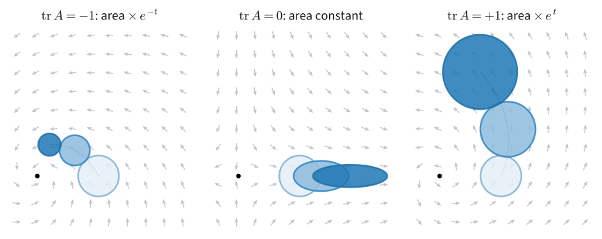
The spiral is the running example in two dimensions. Since \(\mathbf A=-\tfrac12\mathbf{I}+\mathbf K\) and \(\mathbf{I}\) commutes with \(\mathbf K\), \(e^{\mathbf At}=e^{-t/2}e^{t\mathbf K}\), a rotation followed by a shrink by \(e^{-t/2}\). A disc is carried to a disc of \(e^{-t/2}\) times its radius, so its area is multiplied by \(e^{-t}\), and the density along each trajectory rises by \(e^{t}\). Here \(\operatorname{tr}\mathbf A=-1\), so the rate of change of the log-density is again minus the trace. Figure 29.2.4 draws this beside a field that preserves area and one that expands it.
The general case needs one fact about determinants: over a short step the flow map is close to the identity, and the determinant of a matrix close to the identity is governed by its trace.
Lemma. For any square matrix \(\mathbf J\), \(\det(\mathbf{I}+h\mathbf J)=1+h\operatorname{tr}\mathbf J+O(h^2)\).
Proof. In the Leibniz expansion of the determinant, any permutation other than the identity uses at least two off-diagonal entries, each of size \(O(h)\), so it contributes \(O(h^2)\). The identity permutation contributes \(\prod_i(1+hJ_{ii})=1+h\sum_iJ_{ii}+O(h^2)\). \(\blacksquare\)
Proposition (instantaneous change of variables). Let \(\dot{\mathbf{x}}=\mathbf{f}(\mathbf{x},t)\) with \(\mathbf{f}\) continuously differentiable in \((\mathbf{x},t)\) and globally Lipschitz in \(\mathbf{x}\), so that each flow map \(\Phi_t\) is a \(C^1\) bijection with a \(C^1\) inverse (the solution of a \(C^1\) field is \(C^1\) in its initial value (Hairer et al. 1993), and the inverse runs the field backward). Let \(\mathbf{x}(0)\sim p_0\) for a positive differentiable density \(p_0\). Then the density \(p_t\) of \(\mathbf{x}(t)\) exists and is positive, and along each trajectory (Chen et al. 2018)
\[ \frac{d}{dt} \log p_t(\mathbf{x}(t)) = -\operatorname{tr}\!\left(\frac{\partial \mathbf{f}}{\partial \mathbf{x}}\right)\!(\mathbf{x}(t), t). \tag{29.2.8}\]
Proof. The density exists by Equation 29.2.7 applied to the bijection \(\Phi_t\), and it is positive because \(p_0\) is and the Jacobian of a map with a differentiable inverse is nonsingular. Over a short interval the flow advances by the map \(\Phi_{t\to t+h}(\mathbf{x})=\mathbf{x}+\int_t^{t+h}\mathbf{f}(\mathbf{x}(s),s)\,ds\). Differentiating in \(\mathbf{x}\) and using the continuity of \(\mathbf J\), its Jacobian is \(\mathbf{I}+h\mathbf J+o(h)\), where \(\mathbf J=\partial\mathbf{f}/\partial\mathbf{x}\) is evaluated at \((\mathbf{x}(t),t)\) and \(o(h)\) stands for terms that vanish faster than \(h\). Apply Equation 29.2.7 to this one map and expand with the Lemma, which tolerates the perturbation: replacing \(h\mathbf J\) by \(h\mathbf J+o(h)\) changes the determinant only by \(o(h)\). For small \(h\) the determinant is close to \(1\), hence positive, so the absolute value can be dropped:
\[ \log p_{t+h}(\mathbf{x}(t+h)) = \log p_t(\mathbf{x}(t)) - \log\det\!\big(\mathbf{I} + h\mathbf J + o(h)\big) = \log p_t(\mathbf{x}(t)) - h \operatorname{tr} \mathbf J + o(h), \]
using \(\log(1+u)=u+O(u^2)\). Subtract \(\log p_t(\mathbf{x}(t))\), divide by \(h\), and let \(h\to0\). \(\blacksquare\)
The trace of the Jacobian is the divergence of the field, the local rate at which the flow expands volume. Where the field spreads samples apart (\(\operatorname{tr}\mathbf J>0\)) the log-density along each trajectory falls. Where it compresses them, the log-density rises and probability concentrates. Integrating Equation 29.2.8 along a trajectory gives
\[ \log p_T(\mathbf{x}(T)) = \log p_0(\mathbf{x}(0)) - \int_0^T \operatorname{tr}\!\left(\frac{\partial \mathbf{f}}{\partial \mathbf{x}}\right) dt . \tag{29.2.9}\]
The per-layer sum of log-determinants of a discrete flow has become an integral of traces. A model that computes it, by integrating the augmented state \((\mathbf{x},\log p)\) with any ODE solver, is a continuous normalizing flow (CNF). It needs no restriction on the architecture of \(\mathbf{f}\).
For a linear field the trace integral is \(t\operatorname{tr}\mathbf A\), and Equation 29.2.9 compared with Equation 29.2.7 for the map \(e^{\mathbf At}\) says \(\log\det e^{\mathbf At}=t\operatorname{tr}\mathbf A\). This is Jacobi’s formula, which also follows in one line from the eigendecomposition \(\mathbf A=\mathbf V\boldsymbol\Lambda \mathbf V^{-1}\):
\[ \det e^{\mathbf At}=\det\big(\mathbf Ve^{\boldsymbol\Lambda t}\mathbf V^{-1}\big)=\prod_je^{\Lambda_{jj}t}=e^{t\operatorname{tr}\mathbf A} \tag{29.2.10}\]
for diagonalizable \(\mathbf A\), and for every \(\mathbf A\) by continuity, since diagonalizable matrices are dense. For the spiral both sides equal \(e^{-1.5}=0.2231\) at \(t=1.5\). The proposition follows individual trajectories. Stated for the whole density at once instead of along one trajectory, the same law is the continuity equation of fluid mechanics.
29.2.3.2 Checking the Trace Integral
Does the trace integral equal the log-determinant of the flow map, both when the trace is constant and when it varies along the path? For the spiral we can compare with a closed form. Start from \(p_0=\mathcal{N}(\mathbf{0},\mathbf{I})\); a linear map sends it to \(p_t=\mathcal{N}(\mathbf{0},e^{\mathbf At}e^{\mathbf A^\top t})\), which for the spiral is \(\mathcal{N}(\mathbf{0},e^{-t}\mathbf{I})\) because \(e^{t\mathbf K}\) is orthogonal. The cell evaluates this Gaussian at the transported points of four random samples and compares with \(\log p_0(\mathbf{x}_0)-t\operatorname{tr}\mathbf A\).
t = 1.5
X0s = np.random.randn(4, 2)                    # four samples from p_0 = N(0, I)
Et = expm_eig(A, t)
Xts = X0s @ Et.T                               # flow each sample to time t
Sig = Et @ Et.T                                # x(t) ~ N(0, E_t E_t^T)
logp0 = -0.5 * (X0s ** 2).sum(axis=1) - np.log(2 * np.pi)
logpt = (-0.5 * np.einsum('ki,ij,kj->k', Xts, np.linalg.inv(Sig), Xts)
         - 0.5 * np.log(np.linalg.det(Sig)) - np.log(2 * np.pi))
print('log p_t(x(t)), Gaussian formula :', logpt.round(6))
print('log p_0(x_0) - t tr(A) :', (logp0 - t * np.trace(A)).round(6))log p_t(x(t)), Gaussian formula : [-0.662843 -0.441662 -0.537322 -1.246025]
log p_0(x_0) - t tr(A) : [-0.662843 -0.441662 -0.537322 -1.246025]log p_t(x(t)), Gaussian formula : [-0.549271 -3.358567 -1.672318 -1.290884]
log p_0(x_0) - t tr(A) : [-0.549271 -3.358567 -1.672318 -1.290884]log p_t(x(t)), Gaussian formula : [-2.318649 -0.484433 -1.882203 -1.44513 ]
log p_0(x_0) - t tr(A) : [-2.318649 -0.484433 -1.882203 -1.44513 ]log p_t(x(t)), Gaussian formula : [-0.512354 -2.260224 -1.243172 -0.771084]
log p_0(x_0) - t tr(A) : [-0.512354 -2.260224 -1.243172 -0.771084]The two rows agree in every printed digit for any draw, as Jacobi’s formula says they must. A nonlinear field is the real test, because its trace changes along the path. Take the planar field \(\mathbf{f}(\mathbf{x})=\mathbf W_2\tanh(\mathbf W_1\mathbf{x}+\mathbf{b}_1)\) with \(8\) hidden units and random weights. Its Jacobian and trace are explicit:
\[ \mathbf J=\mathbf W_2\,\mathrm{diag}(\mathbf{s})\,\mathbf W_1, \qquad \mathbf{s}=1-\tanh^2(\mathbf W_1\mathbf{x}+\mathbf{b}_1), \qquad \operatorname{tr}\mathbf J=\sum_is_i\,(\mathbf W_1\mathbf W_2)_{ii}, \]
using the cyclic property \(\operatorname{tr}\big(\mathbf W_2\,\mathrm{diag}(\mathbf{s})\,\mathbf W_1\big)=\operatorname{tr}\big(\mathrm{diag}(\mathbf{s})\,\mathbf W_1\mathbf W_2\big)\). The cell integrates the augmented state \((\mathbf{x},\int\operatorname{tr}\mathbf J\,dt)\) with RK4 to \(T=1\) and compares the integral with \(\log|\det D\Phi_T|\), computed from central finite differences of the flow map itself.
H = 8
W1, b1 = np.random.randn(H, 2), np.random.randn(H)
W2 = np.random.randn(2, H) / np.sqrt(H)
field = lambda x: W2 @ np.tanh(W1 @ x + b1)
trJ = lambda x: np.sum((1 - np.tanh(W1 @ x + b1) ** 2)
                       * np.einsum('ij,ji->i', W1, W2))
aug = lambda z: np.append(field(z[:2]), trJ(z[:2]))  # d/dt (x, int tr J)
xa, n = np.random.randn(2), 200
zT = rk4(aug, np.append(xa, 0.0), 1.0, n)
D = np.zeros((2, 2))                           # D Phi_1 by central differences
for j in range(2):
    e = np.zeros(2); e[j] = 1e-5
    D[:, j] = (rk4(field, xa + e, 1.0, n) - rk4(field, xa - e, 1.0, n)) / 2e-5
logdet = np.log(abs(np.linalg.det(D)))
print(f'tr J at x(0) {trJ(xa):+.3f}, at x(1) {trJ(zT[:2]):+.3f}')
print(f'trace integral {zT[2]:+.6f}  log|det D Phi| {logdet:+.6f}  '
f'gap {abs(zT[2] - logdet):.1e}')tr J at x(0) -0.806, at x(1) -1.058
trace integral -0.831245 log|det D Phi| -0.831245 gap 9.9e-11tr J at x(0) -1.184, at x(1) -2.036
trace integral -1.588729 log|det D Phi| -1.588729 gap 2.0e-10tr J at x(0) +0.048, at x(1) -0.002
trace integral +0.021269 log|det D Phi| +0.021269 gap 5.9e-12tr J at x(0) -0.538, at x(1) -0.464
trace integral -0.498645 log|det D Phi| -0.498645 gap 5.8e-11The trace generally takes different values at the two ends of the path, yet the integral and the log-determinant agree to about \(10^{-10}\), and to better than \(10^{-8}\) for any draw of the weights. That gap is the accuracy of the solver and of the finite differences. Nothing in the proposition used linearity.
29.2.3.3 The Hutchinson Trace Estimator
The formula for \(\operatorname{tr}\mathbf J\) above used the structure of a one-layer field. For a general network the trace needs the \(d\) diagonal entries of \(\mathbf J\), which cost \(d\) reverse-mode passes, one per coordinate. At \(d=3072\) that is the cost we set out to avoid. A random projection gives an unbiased estimate from a single pass (Hutchinson 1989).
Proposition (Hutchinson estimator). For any matrix \(\mathbf M\in\mathbb{R}^{d\times d}\) and any random vector \(\boldsymbol\epsilon\in\mathbb{R}^d\) with \(\mathbb{E}[\boldsymbol\epsilon\boldsymbol\epsilon^\top]=\mathbf{I}\), such as a standard Gaussian or a Rademacher vector with independent entries \(\pm1\) of equal probability,
\[ \operatorname{tr}(\mathbf M) = \mathbb{E}\!\left[\boldsymbol{\epsilon}^\top \mathbf M \boldsymbol{\epsilon}\right]. \tag{29.2.11}\]
Proof. \(\mathbb{E}[\boldsymbol\epsilon^\top \mathbf M\boldsymbol\epsilon] =\mathbb{E}[\operatorname{tr}(\mathbf M\boldsymbol\epsilon\boldsymbol\epsilon^\top)] =\operatorname{tr}(\mathbf M\,\mathbb{E}[\boldsymbol\epsilon\boldsymbol\epsilon^\top]) =\operatorname{tr}(\mathbf M)\), by the cyclic property of the trace and its linearity, which lets it commute with the expectation. \(\blacksquare\)
The estimator touches \(\mathbf J\) only through \(\boldsymbol\epsilon^\top \mathbf J\), one vector–Jacobian product, which is one reverse-mode pass through \(\mathbf{f}\) with \(\boldsymbol\epsilon\) as the seed; no Jacobian is formed. For the one-hidden-layer field the product is explicit,
\[ \boldsymbol\epsilon^\top \mathbf J=\big((\boldsymbol\epsilon^\top \mathbf W_2)\odot\mathbf{s}\big)\,\mathbf W_1, \]
and it costs about as much as evaluating \(\mathbf{f}\). A CNF evaluates one such product with every evaluation of the field, so the likelihood costs one additional backward pass per field evaluation (FFJORD, (Grathwohl et al. 2019)).
Can we estimate the trace from vector–Jacobian products alone, without ever forming \(\mathbf J\)? We take a one-hidden-layer field in \(d=50\) with \(64\) hidden units, compute its exact trace from the formula above, and draw \(m=10^5\) Rademacher probes.
d, H, m = 50, 64, 100_000
W1, b1 = np.random.randn(H, d) / np.sqrt(d), 0.1 * np.random.randn(H)
W2 = np.random.randn(d, H) / np.sqrt(H)
x = np.random.randn(d)
s = 1 - np.tanh(W1 @ x + b1) ** 2
tr_exact = np.sum(s * np.einsum('ij,ji->i', W1, W2))
E = np.random.choice([-1.0, 1.0], size=(m, d))  # Rademacher probes, one per row
print(f'exact trace {tr_exact:.4f}')exact trace -0.8364exact trace 0.5969exact trace -0.2224exact trace 0.3409Each framework’s reverse mode computes the rows \(\boldsymbol\epsilon_k^\top \mathbf J\) when its backward pass is seeded with the probes \(\boldsymbol\epsilon_k\) instead of with a loss gradient.
W1t, b1t, W2t = (torch.tensor(w) for w in (W1, b1, W2))
field = lambda x: W2t @ torch.tanh(W1t @ x + b1t)
_, vjp = torch.func.vjp(field, torch.tensor(x))  # reverse mode at x
rows = torch.func.vmap(vjp)(torch.tensor(E))[0]  # row k: eps_k^T J
est = (rows * torch.tensor(E)).sum(dim=1)        # eps_k^T J eps_k
print(f'Hutchinson {est.mean():.4f} +- {est.std() / m ** 0.5:.4f} '
      f'({m} probes, one VJP each)')
Hutchinson -0.8296 +- 0.0160 (100000 probes, one VJP each)xs = tf.constant(np.tile(x, (m, 1))) # m copies of x, one per probe
with tf.GradientTape() as tape:
tape.watch(xs)
ys = tf.tanh(xs @ W1.T + b1) @ W2.T
rows = tape.gradient(ys, xs, output_gradients=tf.constant(E)) # eps_k^T J
est = tf.reduce_sum(rows * E, axis=1)
print(f'Hutchinson {float(tf.reduce_mean(est)):.4f} +- '
f'{float(tf.math.reduce_std(est)) / m ** 0.5:.4f} '
f'({m} probes, one VJP each)')Hutchinson 0.6112 +- 0.0148 (100000 probes, one VJP each)W1j, b1j, W2j = (jnp.array(w) for w in (W1, b1, W2))
field = lambda x: W2j @ jnp.tanh(W1j @ x + b1j)
_, vjp = jax.vjp(field, jnp.array(x)) # reverse mode at x
rows = jax.vmap(vjp)(jnp.array(E))[0] # row k: eps_k^T J
est = (rows * E).sum(axis=1) # eps_k^T J eps_k
print(f'Hutchinson {float(est.mean()):.4f} +- '
f'{float(est.std()) / m ** 0.5:.4f} ({m} probes, one VJP each)')Hutchinson -0.1956 +- 0.0134 (100000 probes, one VJP each)xs = mnp.array(np.tile(x, (m, 1))) # m copies of x, one per probe
xs.attach_grad()
with autograd.record():
ys = mnp.tanh(xs @ mnp.array(W1).T + mnp.array(b1)) @ mnp.array(W2).T
ys.backward(mnp.array(E)) # seed the backward pass with the probes
est = (xs.grad * mnp.array(E)).sum(axis=1) # row k of xs.grad: eps_k^T J
print(f'Hutchinson {float(est.mean()):.4f} +- '
f'{float(est.std()) / m ** 0.5:.4f} ({m} probes, one VJP each)')Hutchinson 0.3479 +- 0.0147 (100000 probes, one VJP each)The estimate lies within a few standard errors of the exact trace, as expected of an unbiased average of \(10^5\) independent probes, and no \(d\times d\) matrix appeared. The estimate is noisy, however. For Rademacher probes one probe has variance \(2\sum_{i\ne j}S_{ij}^2\) with \(\mathbf S=(\mathbf J+\mathbf J^\top)/2\), so the off-diagonal entries set the noise, and the relative error grows with \(d\) when they dominate the diagonal. Here one probe has a standard deviation of about \(4\) to \(5\), while the trace is typically a few tenths in size. A standard error of \(0.01\) would take about \(2\times10^5\) probes.
We can now write a residual network as an Euler program and train it. We can derive the adjoint ODE, recognize backpropagation through a solver as a first-order discretization of it, and decide between storing the states and re-integrating them backward. And we can compute how a flow changes a density with one trace, or one vector–Jacobian product, per step. Everything here moved deterministically. A diffusion model adds fresh noise at every step, and increments that scale like \(\sqrt{h}\) break the Taylor expansions this section relied on. Section 29.3 asks how to integrate such an equation.
29.2.4 Summary
A residual block is an Euler step, and sharing one field while shrinking the step gives a Neural ODE. Its exact flow is invertible and, on \(\mathbb{R}\), order-preserving, so the map \(x\mapsto-x\) needs a second dimension. The gradient of a loss on \(\mathbf{x}(T)\) is the integral of \((\partial\mathbf{f}/\partial\boldsymbol\theta)^\top\mathbf{a}\) along the trajectory, where the adjoint \(\mathbf{a}\) solves a linear ODE backward from \(\nabla\ell(\mathbf{x}(T))\). Backpropagation through Euler is a first-order discretization of that ODE: it is exact for the program and within \(O(h)\) of the gradient of the flow. Re-integrating the state backward saves memory but amplifies a stored error by \(e^{\lambda T}\) for a mode that decays at rate \(\lambda\), from \(10^{-16}\) to about \(5\times10^5\) for \(\lambda=50\) and \(T=1\). Along a trajectory \(\tfrac{d}{dt}\log p_t=-\operatorname{tr}\mathbf J\), so the spiral, with \(\operatorname{tr}\mathbf A=-1\), raises the density along each trajectory by \(e^{t}\). Hutchinson’s estimator obtains the trace from one vector–Jacobian product per probe.
29.2.5 Exercises
[code] The learned field at other step counts. The
#odes-solvers-neural-ode-traincell trains the field with \(N=10\) Euler steps of size \(h=0.1\), and the text found that the endpoint error rises from a few thousandths to about \(0.02\) when the same field is integrated with \(N=100\) or \(N=1000\) steps.- Evaluate the trained
flowwith \(N=1\), \(2\) and \(5\) steps (\(Nh=1\)). Why is the error at \(N=1\) large although ten steps of the same field are accurate to a few thousandths? Which map does one Euler step of the trained field compute? - What does the error at \(N=1000\) measure? Name the two maps whose distance it is, and explain why it does not shrink as \(N\) grows further.
- Integrate the trained field backward from the targets
Ywith \(N=10\), \(100\) and \(1000\) steps of \(\mathbf{x}\leftarrow\mathbf{x}-h\,\mathbf{f}_{\boldsymbol\theta}(\mathbf{x})\) and compare the result withX. The forward–backward round trip of the text went to zero like \(1/N\); this error settles near \(0.03\). Why? Hint: at large \(N\) the backward integration applies the exact inverse flow to the ellipse, not to the ten-step image of the circle. - Retrain with \(N=1\) and with \(N=2\), and repeat (a). Which of the three trained fields comes closest to its own time-one flow?
- Evaluate the trained
[code] What a flow cannot represent. ● Two trajectories of a field with Lipschitz constant \(L\) satisfy \(e^{-Lt}\|\mathbf{x}-\mathbf{y}\|\le\|\Phi_t(\mathbf{x})-\Phi_t(\mathbf{y})\|\le e^{Lt}\|\mathbf{x}-\mathbf{y}\|\) (1), and Section 29.2.1.2 showed that no flow on \(\mathbb{R}\) reverses order (Dupont et al. 2019).
- Let \(d=1\). Use the lower bound to give a second proof that \(\Phi_T\) is strictly increasing, and show that \(\Phi_T(1)-\Phi_T(-1)\ge2e^{-LT}\). Which of the two statements, order or distance, does the proposition of the text give, and which needs the bound?
- The training example carries the circle points \((0,\pm1)\), which are \(2\) apart, to \((1.5,\pm0.4)\), which are \(0.8\) apart. Show that the exact time-\(T\) flow of a field with Lipschitz constant \(L\) can do this only if \(LT\ge\ln2.5\approx0.92\), whereas the long axis, stretched from \(2\) to \(2.4\), gives only \(LT\ge\ln1.2\). A one-hidden-layer tanh field has \(L\le\|\mathbf W_2\|_2\|\mathbf W_1\|_2\) because \(\tanh\) is \(1\)-Lipschitz. Compute this bound for the trained field and check the inequality.
- Embed \(\mathbb{R}\) in \(\mathbb{R}^2\) as \(x\mapsto(x,0)\). Show that every linear field \(\dot{\mathbf{x}}=\mathbf B\mathbf{x}\) whose time-one map sends \((x,0)\) to \((-x,0)\) for every \(x\) has \(e^{\mathbf B}=-\mathbf{I}\). Hint: an eigenvalue \(-1\) of \(e^{\mathbf B}\) comes from an eigenvalue \(\mu\) of \(\mathbf B\) with \(e^{\mu}=-1\), which is not real. Find such a field whose trajectories are ellipses rather than circles.
- Change the training cell to fit the map \(x\mapsto-x\) on \(64\) evenly spaced points of \([-1,1]\) with a field of input and output dimension \(1\) and \(N=10\) steps. What does the trained model output, and why does the loss settle at a value you can predict before training? Repeat with a field of dimension \(2\), inputs \((x,0)\), and the loss on the first coordinate.
- Train the one-dimensional model once more with \(N=1\) and \(h=1\), and evaluate it with \(N=1\) and with \(N=100\) steps of size \(h=0.01\). Relate the two results to the proposition and to the condition \(hL<1\).
Adjoint with a running loss. ● The adjoint equations Equation 29.2.4 and Equation 29.2.5 treat a loss on the endpoint. Regularizers such as the kinetic energy \(\int_0^T\|\mathbf{f}(\mathbf{x}(t),\boldsymbol\theta,t)\|^2\,dt\) of Finlay et al. (2020) accumulate a cost along the trajectory. Let
\[ \mathcal{L} = \ell_T(\mathbf{x}(T)) + \int_0^T \ell(\mathbf{x}(t), \boldsymbol\theta, t)\,dt . \]
- Extend the variational proof of Equation 29.2.4 to show that the adjoint acquires a source term, \(\dot{\mathbf{a}} = -(\partial\mathbf{f}/\partial\mathbf{x})^\top\mathbf{a} - \nabla_{\mathbf{x}}\ell\) with \(\mathbf{a}(T) = \nabla\ell_T(\mathbf{x}(T))\), and that \(\partial\mathcal{L}/\partial\boldsymbol\theta = \int_0^T \big((\partial\mathbf{f}/\partial\boldsymbol\theta)^\top\mathbf{a} + \nabla_{\boldsymbol\theta}\ell\big)\,dt\).
- Finlay et al. (2020) instead append a coordinate \(E\) with \(\dot{E} = \ell\) and \(E(0) = 0\) to the state, and add \(E(T)\) to the endpoint loss. Apply Equation 29.2.4 to the augmented state and show that it reproduces (a).
- For the kinetic energy, \(\ell = \|\mathbf{f}\|^2\). Write \(\nabla_{\mathbf{x}}\ell\) as a vector–Jacobian product. How many reverse-mode passes through \(\mathbf{f}\) does one step of the adjoint ODE then require?
[code] Reconstructing the trajectory backward. ● The continuous adjoint can avoid storing the forward states by integrating \(\mathbf{x}(t)\) backward from \(\mathbf{x}(T)\) alongside \(\mathbf{a}(t)\), and Section 29.2.2 quoted the resulting drift \(e^{\lambda T}\delta\).
- For \(\dot{x}=-\lambda x\) with \(\lambda>0\), an error \(\delta\) in the stored \(x(T)\) causes an error in the reconstructed \(x(0)\). Derive it.
- Let \(\mathbf R\) be the rotation by \(0.6\) radians and \(\mathbf B=\mathbf R\,\mathrm{diag}(-50,-1)\,\mathbf R^\top\). Integrate \(\dot{\mathbf{x}}=\mathbf B\mathbf{x}\) from \((1,1)\) to time \(T\) with
rk4and \(2000\) steps, then integrate the field \(-\mathbf B\mathbf{x}\) from the result for the same time. Report the reconstruction error for \(T=0.25\), \(0.5\), \(1\) and \(2\), and compare its growth with (a), taking \(\delta\) to be the double-precision rounding error \(\approx10^{-16}\). Repeat with \(\mathrm{diag}(-50,-1)\) itself. Why does the diagonal matrix reconstruct far more accurately? - Activation checkpointing (Section 5.7.3.3) stores the state at the start of each segment of the trajectory. A hybrid scheme reconstructs the states within a segment by integrating backward from the checkpoint at its end. For the matrix \(\mathbf B\) of (b), what is the longest segment duration for which the error of (a) stays below \(10^{-8}\)?
Log-determinant of a residual step. ● The instantaneous change of variables Equation 29.2.8 is a limit of infinitesimal steps. A finite residual step \(F(\mathbf{x})=\mathbf{x}+\mathbf{g}(\mathbf{x})\) needs its exact log-determinant, as in the invertible residual networks of Behrmann et al. (2019) .
Let \(\mathbf{g}\) be Lipschitz with constant \(c<1\). For \(d=1\) the one-line argument of Section 29.2.1.2 (an Euler step is increasing when \(hL<1\)) shows that \(F\) is strictly increasing, hence injective. For general \(d\), write \(F(\mathbf{x})=\mathbf{y}\) as a fixed-point equation for \(\mathbf{x}\) and use the Banach fixed-point theorem, as in the proof of Picard–Lindelöf, to show that \(F\) is a bijection of \(\mathbb{R}^d\). How fast does the fixed-point iteration converge?
Show that \(\|\mathbf J_{\mathbf{g}}\|\le c\), where \(\mathbf J_{\mathbf{g}}\) is the Jacobian of \(\mathbf{g}\), and use the eigenvalues of \(\mathbf J_{\mathbf{g}}\) to show that
\[ \log\det(\mathbf{I} + \mathbf J_{\mathbf{g}}) = \sum_{k=1}^\infty \frac{(-1)^{k+1}}{k}\operatorname{tr}\big(\mathbf J_{\mathbf{g}}^k\big). \]
An Euler step has \(\mathbf{g}=h\mathbf{f}\) and \(\mathbf J_{\mathbf{g}}=h\mathbf J\). Compare \(\log\det(\mathbf{I}+h\mathbf J)\) with the term \(h\operatorname{tr}\mathbf J\) that Equation 29.2.9 accumulates per step. How large is the difference per step, and how large is it in total over \(T/h\) steps?
The Hutchinson estimator Equation 29.2.11 estimates \(\operatorname{tr}(\mathbf J_{\mathbf{g}}^k)\) by \(\boldsymbol{\epsilon}^\top \mathbf J_{\mathbf{g}}^k\boldsymbol{\epsilon}\). How many vector–Jacobian products per probe does the series truncated after \(n\) terms cost?
[code] Variance of the Hutchinson estimator. ● The estimator Equation 29.2.11 estimates \(\operatorname{tr}\mathbf M\) by \(\boldsymbol{\epsilon}^\top \mathbf M\boldsymbol{\epsilon}\) for a single probe \(\boldsymbol{\epsilon}\). Let \(\mathbf S=(\mathbf M+\mathbf M^\top)/2\), so that \(\boldsymbol{\epsilon}^\top \mathbf M\boldsymbol{\epsilon}=\boldsymbol{\epsilon}^\top \mathbf S\boldsymbol{\epsilon}\).
- Show that the variance of \(\boldsymbol{\epsilon}^\top \mathbf M\boldsymbol{\epsilon}\) is \(2\|\mathbf S\|_F^2\) for Gaussian probes and \(2\sum_{i\neq j}S_{ij}^2\) for Rademacher probes. For which matrices is a single Rademacher probe exact?
- Form the Jacobian \(\mathbf J=\mathbf W_2\,\mathrm{diag}(\mathbf{s})\,\mathbf W_1\) of the field in the
#mdl-neural-odes-the-hutchinson-trace-estimator-1cell explicitly (it is \(50\times50\)), evaluate both variances, and compare the Rademacher value with \(m\) times the square of the standard error that the next cell printed. How many probes does each distribution need for a standard error of \(0.01\)? - In a CNF, \(\mathbf M\) is the Jacobian \(\partial\mathbf{f}/\partial\mathbf{x}\) in dimension \(d\). Suppose that all entries have comparable magnitude. How does the relative standard error \(\sqrt{\textrm{Var}}/|\operatorname{tr}\mathbf M|\) of one probe scale with \(d\) when the diagonal entries share one sign, and when their signs are random?
[code] Discrete and continuous adjoints. ●● Backpropagation through a solver differentiates the executed program, whereas a solver applied to the adjoint ODE Equation 29.2.4 approximates the gradient of the exact flow (Kidger 2022). Compare the two recursions step by step for an autonomous field with Jacobian \(\mathbf J(\mathbf{x})=\partial\mathbf{f}/\partial\mathbf{x}\) and forward states \(\mathbf{x}_k\).
- For forward Euler, the discrete adjoint Equation 29.2.6 computes \(\mathbf{a}_k=(\mathbf{I}+h\mathbf J(\mathbf{x}_k))^\top\mathbf{a}_{k+1}\), whereas an explicit Euler step of the adjoint ODE from \(t_{k+1}\) back to \(t_k\) computes \(\mathbf{a}_k=\mathbf{a}_{k+1}+h\mathbf J(\mathbf{x}_{k+1})^\top\mathbf{a}_{k+1}\). Bound the difference of the two updates for a smooth \(\mathbf{f}\). For a linear field the two coincide; what then produces the gap that the
#mdl-neural-odes-backpropagation-as-the-discrete-adjoint-1cell prints? For the scalar program \(x_N=(1+h\theta)^Nx_0\) the text found the gradient \(T\,x_N^2/(1+h\theta)\); show that this is what the recursion computes. - Differentiate one Heun step \(\mathbf{x}_{k+1}=\mathbf{x}_k+\tfrac{h}{2}\big[\mathbf{f}(\mathbf{x}_k)+\mathbf{f}(\mathbf{u}_k)\big]\) with \(\mathbf{u}_k=\mathbf{x}_k+h\mathbf{f}(\mathbf{x}_k)\) to obtain its discrete adjoint recursion. Show that this recursion is a Heun step of the adjoint ODE from \(t_{k+1}\) to \(t_k\) in which \(\mathbf J(\mathbf{x}_{k+1})\) is replaced by \(\mathbf J(\mathbf{u}_k)\). At which order in \(h\) do the two updates differ?
- For a linear field \(\mathbf{f}(\mathbf{x})=\mathbf A\mathbf{x}\), one RK4 step multiplies the state by \(R(h\mathbf A)\), where \(R(z)=1+z+z^2/2+z^3/6+z^4/24\) is the RK4 stability polynomial (2). Show that the discrete adjoint of RK4 is an RK4 step of the adjoint ODE.
- Replace the Euler step of
loss_and_grad_unrolledby an RK4 step, and compute the gradient of the unrolled loss by central finite differences instead of a hand-written backward sweep. Measure its gap to the continuous-adjoint gradientg_contfor \(n=5\), \(10\), \(20\), \(40\) and \(80\) steps. The trapezoid rule that computesg_contusesn_quad = 2000intervals and is accurate only to about \(10^{-7}\), so refine it first. Which slope do you measure? Which order does the gradient computed through a solver of order \(p\) inherit?
- For forward Euler, the discrete adjoint Equation 29.2.6 computes \(\mathbf{a}_k=(\mathbf{I}+h\mathbf J(\mathbf{x}_k))^\top\mathbf{a}_{k+1}\), whereas an explicit Euler step of the adjoint ODE from \(t_{k+1}\) back to \(t_k\) computes \(\mathbf{a}_k=\mathbf{a}_{k+1}+h\mathbf J(\mathbf{x}_{k+1})^\top\mathbf{a}_{k+1}\). Bound the difference of the two updates for a smooth \(\mathbf{f}\). For a linear field the two coincide; what then produces the gap that the
Checkpointing arithmetic. ● A forward pass of \(N\) Euler steps is differentiated by the discrete adjoint Equation 29.2.6, whose backward sweep needs \(\mathbf{x}_k\) at step \(k\).
- Storing every state holds \(N\) states and recomputes nothing. Suppose instead that only every \(k\)-th state is stored as a checkpoint, and that when the backward sweep enters a segment of \(k\) steps, the segment is recomputed forward from its checkpoint and its states are held until the sweep leaves it. How many states are held at the peak, and how many extra forward steps are computed in total?
- Minimize the peak over \(k\). Show that the minimum is near \(k=\sqrt N\), and that the extra work is about one forward pass whatever \(k\) is. For \(N=1000\), compare the peak with the \(1000\) states of full storage.
- Recursive checkpointing applies the same idea inside each segment and holds \(O(\log N)\) states at the cost of \(O(\log N)\) forward passes (Griewank 1992). Compare it with the continuous adjoint, whose memory is constant but whose backward re-integration amplifies an error by \(e^{\lambda T}\) on \(\dot{x}=-\lambda x\). For which \(\lambda T\) does re-integration from a state stored in single precision (\(\delta\approx6\times10^{-8}\)) lose all accuracy?
[code] Liouville’s formula. ●● The instantaneous change of variables followed a density along a trajectory. This exercise proves it a second way, through the Jacobian \(\mathbf M(t)=D\Phi_t(\mathbf{x}_0)\) of the flow map itself.
- Differentiate \(\tfrac{d}{dt}\Phi_t(\mathbf{x}_0)=\mathbf{f}(\Phi_t(\mathbf{x}_0),t)\) with respect to \(\mathbf{x}_0\) to obtain the variational equation \(\dot{\mathbf M}=\mathbf J(\mathbf{x}(t),t)\,\mathbf M\) with \(\mathbf M(0)=\mathbf{I}\).
- Prove Jacobi’s formula \(\tfrac{d}{dt}\det \mathbf M=\operatorname{tr}(\mathbf M^{-1}\dot{\mathbf M})\det \mathbf M\) for invertible \(\mathbf M(t)\). Hint: write \(\det \mathbf M(t+h)=\det \mathbf M(t)\,\det\big(\mathbf{I}+h\mathbf M^{-1}\dot{\mathbf M}+O(h^2)\big)\) and use the Lemma.
- Conclude that \(\log|\det D\Phi_T(\mathbf{x}_0)|=\int_0^T\operatorname{tr}\mathbf J(\mathbf{x}(t),t)\,dt\), and derive Equation 29.2.9 from the discrete change of variables Equation 29.2.7 applied to the bijection \(\Phi_T\). For a linear field the result is Equation 29.2.10, Jacobi’s formula.
- Integrate \(\dot{\mathbf M}=\mathbf J\mathbf M\) with RK4 alongside the \(8\)-unit tanh field of the
#mdl-neural-odes-checking-the-trace-integral-1cell (re-create its weights, since the Hutchinson cells reuse the names) and compare \(\log|\det \mathbf M(1)|\) with the two numbers that cell prints.