%matplotlib inline
from d2l import torch as d2l
import numpy as np
import torch29.1 Ordinary Differential Equations and Numerical Solvers
A continuous-time model is not yet an executable model. The differential equation specifies a trajectory, but generation requires a numerical method that replaces this trajectory by finitely many updates. A stable continuous system can therefore yield a poor computation if the step size is too large, and a higher-order method can reduce error without changing the learned vector field. For example, the exact solution of \(\dot{x}=-50x\) decays, but forward Euler with step \(h=0.05\) grows because its update factor is \(1-50h=-1.5\); with \(h=0.01\) it decays. Solver analysis explains this difference.
We first define vector fields and the conditions under which they generate a unique flow. Linear systems then show how eigenvalues govern asymptotic stability. This analysis supplies the test problems used to compare Euler, Runge–Kutta, and implicit methods. Only after separating the exact flow from its numerical approximation do we interpret residual updates as Euler steps, derive continuous and discrete adjoints, and track densities in continuous normalizing flows. The stochastic Euler method appears in Section 29.2.3.2; the probability-flow ODE appears in Section 29.3.
We lean on Section 24.2 (eigenvalues and eigenvectors; that section already defined the matrix exponential, and here we prove its properties), Section 25.2 (Jacobians, Taylor expansion), Section 25.3 (reverse-mode AD as vector–Jacobian products), Section 25.4 (the integrals being approximated), and Section 27.1 (the change-of-variables formula for densities). The numerical demonstrations use NumPy until the Neural ODE training example.
%matplotlib inline
from d2l import tensorflow as d2l
import numpy as np
import tensorflow as tf%matplotlib inline
from d2l import jax as d2l
import jax
from jax import numpy as jnp
import numpy as np%matplotlib inline
from d2l import mxnet as d2l
from mxnet import autograd, gluon, init, np as mnp, npx
from mxnet.gluon import nn
import numpy as np
npx.set_np()29.1.1 Vector Fields, Trajectories, and Well-Posedness
29.1.1.1 Velocity Fields and Integral Curves
An initial-value problem specifies a velocity rule and a starting point:
\[ \dot{\mathbf{x}}(t) = \mathbf{f}(\mathbf{x}(t), t), \qquad \mathbf{x}(0) = \mathbf{x}_0, \tag{29.1.1}\]
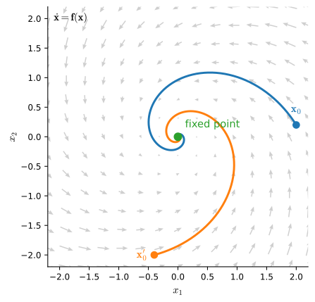
where \(\mathbf{x}(t) \in \mathbb{R}^d\) is the state, the dot is the time derivative, and \(\mathbf{f} : \mathbb{R}^d \times \mathbb{R} \to \mathbb{R}^d\) is a vector field: a function that attaches an arrow to every point. A trajectory (or integral curve) is a differentiable path whose tangent matches the field everywhere: at each instant, the particle moves with exactly the velocity the field prescribes at its current location. When \(\mathbf{f}\) does not depend on \(t\) we call the system autonomous; the arrows are frozen and only the particle moves. Figure 29.1.1 shows a grid of field vectors and trajectories tangent to them.
Integrating both sides of Equation 29.1.1 from \(0\) to \(t\) (Section 25.4) gives the equivalent integral form
\[ \mathbf{x}(t) = \mathbf{x}_0 + \int_0^t \mathbf{f}(\mathbf{x}(s), s)\,ds, \tag{29.1.2}\]
which trades the derivative for an accumulation of velocities. This form serves two purposes: it defines the fixed-point equation used in the existence theorem below, and it is the expression approximated by numerical solvers; Euler’s method is the left-endpoint Riemann sum of this very integral.
Two examples establish the notation. For \(\dot{x} = -x\), the rule “move toward zero at a speed proportional to displacement” is solved by \(x(t) = e^{-t} x_0\): exponential decay, the prototype of a contracting mode. For the rotational field \(\dot{\mathbf{x}} = \left(\begin{smallmatrix}0&-1\\1&0\end{smallmatrix}\right)\mathbf{x}\), the velocity is always perpendicular to the position, so \(\tfrac{d}{dt}\|\mathbf{x}\|^2 = 2\,\mathbf{x}^\top\dot{\mathbf{x}} = 0\) and trajectories are circles traversed at constant angular speed: pure rotation, the prototype of an oscillating mode. The field of Figure 29.1.1 is exactly the sum of these two behaviors, and its eigenvalues \(-0.5 \pm i\) encode both behaviors.
29.1.1.2 The Flow Map
Fix the field and vary the starting point: for an autonomous system, write \(\Phi_t(\mathbf{x}_0) = \mathbf{x}(t)\) for the solution at time \(t\) started at \(\mathbf{x}_0\). This flow map \(\Phi_t : \mathbb{R}^d \to \mathbb{R}^d\) moves every point of space forward \(t\) seconds along its arrows, and it composes the way time does:
\[ \Phi_0 = \mathrm{id}, \qquad \Phi_{t+s} = \Phi_t \circ \Phi_s . \]
Flowing for \(s\) seconds and then \(t\) more is the same as flowing for \(t+s\), whenever all three solutions exist. This holds because the field is frozen in time: the second leg starts from \(\Phi_s(\mathbf{x}_0)\) and follows the same rule. If solutions exist uniquely both forward and backward over the relevant interval, taking \(s=-t\) gives \(\Phi_t \circ \Phi_{-t}=\mathrm{id}\), so \(\Phi_t\) is a bijection with inverse \(\Phi_{-t}\). A field whose solutions exist for every positive and negative time therefore generates a one-parameter group of bijections. This provides the basis for an invertible generative flow: push noise forward through a learned field to get data, and integrate backward to recover the noise (and, as we will see in Section 29.1.5, its likelihood). The next subsection states sufficient conditions for existence and uniqueness.
29.1.1.3 Existence and Uniqueness
Before building on this, we need to know that exactly one trajectory passes through each starting point. The right hypothesis is that the field does not change too abruptly from point to point.
Proposition (Picard–Lindelöf). Let \(\mathbf{f}(\mathbf{x}, t)\) be continuous in \(t\) and Lipschitz in \(\mathbf{x}\): there is an \(L\) with
\[ \|\mathbf{f}(\mathbf{x}, t) - \mathbf{f}(\mathbf{y}, t)\| \le L\,\|\mathbf{x} - \mathbf{y}\| \qquad \textrm{for all } \mathbf{x}, \mathbf{y}, t. \]
Then the initial-value problem Equation 29.1.1 has exactly one solution on \([0, T]\), for every \(\mathbf{x}_0\) and every \(T\) (Coddington and Levinson 1955).
Proof sketch (the integral operator is a contraction). A path \(\boldsymbol{\varphi}\) solves Equation 29.1.1 iff it is a fixed point of the Picard operator built from the integral form Equation 29.1.2,
\[ (P\boldsymbol{\varphi})(t) = \mathbf{x}_0 + \int_0^t \mathbf{f}(\boldsymbol{\varphi}(s), s)\,ds . \]
For two candidate paths on a short interval \([0, \delta]\),
\[ \|(P\boldsymbol{\varphi})(t) - (P\boldsymbol{\psi})(t)\| \le \int_0^t \|\mathbf{f}(\boldsymbol{\varphi}(s), s) - \mathbf{f}(\boldsymbol{\psi}(s), s)\|\,ds \le L\,\delta \cdot \max_{s \le \delta}\|\boldsymbol{\varphi}(s) - \boldsymbol{\psi}(s)\| , \]
so once \(\delta < 1/L\) the operator \(P\) shrinks the distance between any two paths by a fixed factor: it is a contraction, and by the Banach fixed-point theorem a contraction on a complete space has exactly one fixed point (iterate \(P\) from anywhere; the iterates form a Cauchy sequence, and two distinct fixed points would have to be strictly closer to each other than they are). Completeness is what turns the Cauchy sequence into a solution: the space \(C([0, \delta])\) of continuous paths under the sup norm is complete, so the iterates converge uniformly to a continuous fixed point. That settles \([0, \delta]\); restart at \(t = \delta\) and repeat to cover all of \([0, T]\).
Iterating \(P\) from the constant path is Picard iteration; here it is once by hand. For \(\dot{x} = x\), \(x_0 = 1\): starting from \(\varphi_0 \equiv 1\),
\[ \varphi_1(t) = 1 + t, \qquad \varphi_2(t) = 1 + t + \tfrac{t^2}{2}, \qquad \varphi_3(t) = 1 + t + \tfrac{t^2}{2} + \tfrac{t^3}{6}, \;\;\ldots \]
These are the partial sums of \(e^t\). Each Picard iteration adds one Taylor term.
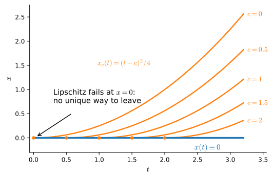
These hypotheses are a convenient sufficient package, not individually necessary conditions. Two standard counterexamples show the failures that they are designed to rule out. Uniqueness can fail without Lipschitz. The field \(\dot{x} = \sqrt{|x|}\) has slope \(\to \infty\) near \(x = 0\) (no finite \(L\) works there), and the initial value \(x_0 = 0\) admits infinitely many solutions: \(x(t) \equiv 0\) is one, and for every waiting time \(c \ge 0\),
\[ x_c(t) = \begin{cases} 0, & t \le c, \\ (t - c)^2/4, & t > c \end{cases} \]
is another: it remains at the origin for \(c\) seconds and then becomes positive (check: \(\dot{x}_c = (t-c)/2 = \sqrt{x_c}\) for \(t > c\)). Each departure time gives a distinct solution, so the initial-value problem is not unique (Figure 29.1.2).
Global existence fails without a growth bound. The field \(\dot{x} = x^2\) is Lipschitz on every bounded set but not globally, and from \(x_0 > 0\), separation of variables gives
\[ x(t) = \frac{x_0}{1 - x_0 t}, \]
which diverges at the finite time \(t = 1/x_0\): the growth rate itself grows superlinearly until a singularity forms. The solution exists only locally, on \([0, 1/x_0)\), which is all that local Lipschitz continuity can promise.
For deep learning the theorem supplies a well-posed continuous model. A neural field \(\mathbf{f}_\theta\) built from linear maps and Lipschitz activations (\(\tanh\), ReLU, GELU) is globally Lipschitz (a composition of globally Lipschitz maps is globally Lipschitz, with constant at most the product of the weight norms and the activations’ Lipschitz constants), which is exactly the global-\(L\) hypothesis of the proposition above. So a Neural ODE (Section 29.1.4) is well-posed: through every input there is exactly one trajectory, distinct inputs can never collide (two trajectories meeting at time \(t\) would be two solutions of the same final-value problem run backward), and the exact map \(\Phi_T\) is a bijection whenever solutions exist uniquely in both time directions over the interval. A finite numerical update, including a residual block interpreted as an Euler step, need not be injective.
29.1.2 Linear ODEs and Stability
29.1.2.1 The Matrix Exponential
One family of ODEs can be solved in closed form, and it is the family that explains all the others locally: the linear system
\[ \dot{\mathbf{x}} = A\mathbf{x}, \qquad \mathbf{x}(0) = \mathbf{x}_0, \qquad A \in \mathbb{R}^{d \times d}. \]
In one dimension, \(\dot{x} = ax\) is solved by \(e^{at} x_0\), which motivates defining a matrix exponential with the analogous solution formula. Define, for any square matrix \(B\), the matrix exponential by the same power series that defines \(e^z\):
\[ e^{B} = \sum_{k=0}^{\infty} \frac{B^k}{k!} = I + B + \frac{B^2}{2} + \frac{B^3}{6} + \cdots . \tag{29.1.3}\]
The series converges for every matrix: term by term, \(\|B^k\| \le \|B\|^k\) (the operator norm is submultiplicative), so the series is dominated by the scalar series for \(e^{\|B\|}\), which converges absolutely.
Proposition (the matrix exponential solves linear ODEs). \(\mathbf{x}(t) = e^{At}\mathbf{x}_0\) is the unique solution of \(\dot{\mathbf{x}} = A\mathbf{x}\), \(\mathbf{x}(0) = \mathbf{x}_0\).
Proof. Differentiate the series Equation 29.1.3 with \(B = At\) term by term (legitimate: on any bounded \(t\)-interval the differentiated series still converges uniformly, by the same domination):
\[ \frac{d}{dt} e^{At} = \sum_{k=1}^{\infty} \frac{A^k\, t^{k-1}}{(k-1)!} = A \sum_{j=0}^{\infty} \frac{(At)^j}{j!} = A\, e^{At}. \]
So \(\mathbf{x}(t) = e^{At}\mathbf{x}_0\) satisfies the ODE, and at \(t = 0\) the series collapses to \(I\), so \(\mathbf{x}(0) = \mathbf{x}_0\). Uniqueness is Picard–Lindelöf: the field \(\mathbf{x} \mapsto A\mathbf{x}\) is Lipschitz with \(L = \|A\|\). \(\blacksquare\)
An infinite series of matrix powers sounds unwieldy, but the eigendecomposition of Section 24.2 collapses it to \(d\) scalar exponentials.
Proposition (matrix exponential by eigendecomposition). If \(A = V \Lambda V^{-1}\) with \(\Lambda = \mathrm{diag}(\lambda_1, \ldots, \lambda_d)\), then
\[ e^{At} = V e^{\Lambda t} V^{-1}, \qquad e^{\Lambda t} = \mathrm{diag}\!\left(e^{\lambda_1 t}, \ldots, e^{\lambda_d t}\right). \tag{29.1.4}\]
Proof. Powers telescope: \((At)^k = V (\Lambda t)^k V^{-1}\), because each adjacent \(V^{-1} V\) cancels. Summing the series Equation 29.1.3 and pulling \(V, V^{-1}\) out of the sum gives \(e^{At} = V\left(\sum_k (\Lambda t)^k / k!\right) V^{-1}\). The inner sum is the exponential of a diagonal matrix, which is diagonal with entries \(\sum_k (\lambda_i t)^k / k! = e^{\lambda_i t}\). \(\blacksquare\)
The formula is a decoupling statement. Expand the start point in the eigenbasis, \(\mathbf{x}_0 = \sum_i c_i \mathbf{v}_i\); then
\[ \mathbf{x}(t) = \sum_{i=1}^{d} c_i\, e^{\lambda_i t}\, \mathbf{v}_i : \]
along each eigendirection the system is the scalar equation \(\dot{x} = \lambda_i x\) we already solved, evolving independently of the others. Eigenvectors are the directions in which a linear ODE is one-dimensional; the \(e^{\lambda_i t}\) are its modes.
29.1.2.2 Stability from Eigenvalues
Each mode \(e^{\lambda_i t}\) with \(\lambda_i = a_i + i b_i\) has magnitude \(|e^{\lambda_i t}| = e^{a_i t}\): the real part sets growth or decay, the imaginary part sets rotation. Reading Equation 29.1.4 mode by mode gives the following classification:
- \(\operatorname{Re}\lambda_i < 0\) for all \(i\): every mode decays, and \(\mathbf{x}(t) \to \mathbf{0}\) from every start: the origin is asymptotically stable, with decay rate set by the slowest mode, \(\max_i \operatorname{Re}\lambda_i\).
- \(\operatorname{Re}\lambda_i > 0\) for some \(i\): that mode grows exponentially, and almost every trajectory escapes: unstable.
- \(\operatorname{Im}\lambda_i \neq 0\): the conjugate pair contributes \(e^{a t}(\cos bt, \sin bt)\) terms: rotation, decaying or growing with the sign of \(a\).
The rotation case extends the eigenvalue analysis of Section 24.2.1.3.3 run in continuous time. On the invariant plane of a conjugate pair \(a \pm ib\), the matrix \(A\) acts as the block \(\left(\begin{smallmatrix}a & -b\\ b & \phantom{-}a\end{smallmatrix}\right)\) of Equation 24.2.7. Write it as \(aI + bJ\) with \(J = \left(\begin{smallmatrix}0 & -1\\ 1 & \phantom{-}0\end{smallmatrix}\right)\); since \(J^2 = -I\), the exponential series splits into cosine and sine parts, \(e^{(aI + bJ)t} = e^{at}(\cos bt \, I + \sin bt \, J)\), which is scaling by \(e^{at}\) composed with rotation by \(bt\). Where the iterated matrix of Section 24.2.1.3.3 turned by a fixed angle \(\theta\) per step, the flow turns at angular velocity \(b\): this is the spiral, and it is exactly where the \(e^{at}(\cos bt, \sin bt)\) terms above come from.
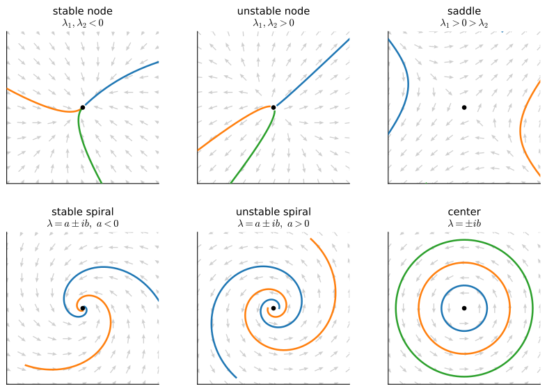
In two dimensions, these cases correspond to standard phase portraits (Figure 29.1.3). For a saddle with real eigenvalues of opposite signs, trajectories approach along the stable eigendirection and diverge along the unstable one. The stable spiral is the field of Figure 29.1.1 (\(\lambda = -0.5 \pm i\): rotate while decaying); the center is our rotation warm-up.
| eigenvalues of \(A\) (\(2\times 2\)) | portrait | behavior |
|---|---|---|
| real, both negative | stable node | monotone decay |
| real, both positive | unstable node | monotone growth |
| real, opposite signs | saddle | decay in, escape out |
| complex pair, \(\operatorname{Re}\lambda < 0\) | stable spiral | decaying oscillation |
| complex pair, \(\operatorname{Re}\lambda > 0\) | unstable spiral | growing oscillation |
| purely imaginary pair | center | closed orbits |
(When \(A\) is defective, i.e. not diagonalizable (Section 24.2), generalized modes acquire polynomial factors \(t^k e^{\lambda t}\). For nonzero real parts the exponential still determines the asymptotic verdict. On the imaginary axis, however, a nontrivial Jordan block can cause polynomial growth and must be classified separately.)
29.1.2.3 Linearization at Fixed Points
Nonlinear fields inherit all of this locally. A fixed point of an autonomous system is a state \(\mathbf{x}^\star\) with \(\mathbf{f}(\mathbf{x}^\star) = \mathbf{0}\): the particle parked there never moves. For a small displacement \(\boldsymbol{\delta}(t) = \mathbf{x}(t) - \mathbf{x}^\star\), Taylor expansion (Section 25.2) gives
\[ \dot{\boldsymbol{\delta}} = \mathbf{f}(\mathbf{x}^\star + \boldsymbol{\delta}) = J\,\boldsymbol{\delta} + O(\|\boldsymbol{\delta}\|^2), \qquad J = \frac{\partial \mathbf{f}}{\partial \mathbf{x}}(\mathbf{x}^\star), \]
so near the fixed point the dynamics are the linear system \(\dot{\boldsymbol{\delta}} = J \boldsymbol{\delta}\), and the eigenvalues of the Jacobian at the fixed point decides local stability by the same classification. (This is rigorous whenever no eigenvalue lies on the imaginary axis, by the Hartman–Grobman theorem (Hartman 1960; Grobman 1959); on the axis, the neglected quadratic terms get a vote.) Write the damped pendulum \(\ddot{\theta} = -\sin\theta - \gamma\dot{\theta}\) as a first-order system in \((\theta, \dot{\theta})\). It has Jacobian eigenvalues with negative real part at the hanging rest point \((0, 0)\) (a stable spiral, the ring-down of a released pendulum) and a saddle at the inverted balance \((\pi, 0)\), analogous to balancing a pencil on its tip: only a measure-zero set of initial conditions remains there. The same computation is the working stability tool of this whole chapter, applied to a trained network’s dynamics or to the mean of the Ornstein–Uhlenbeck process (Section 29.2.4, whose deterministic skeleton is exactly the contracting mode \(\dot{x} = -\theta x\)).
Let us compute all of this. The cell builds \(e^{At}\) for the spiral field of Figure 29.1.1 three independent ways: the eigendecomposition formula Equation 29.1.4, the truncated series Equation 29.1.3, and the compounding limit \((I + tA/n)^n\), which is the forward-Euler approximation introduced in the next section. It then checks the eigenvalue prediction that \(\|\mathbf{x}(t)\|\) decays exactly like \(e^{-t/2}\) (the rotation part of this particular \(A\) is norm-preserving).
A = np.array([[-0.5, -1.0], [1.0, -0.5]])      # spiral sink: eigenvalues -0.5 +- i
t = 2.0
lam, V = np.linalg.eig(A)                      # A = V diag(lam) V^{-1}
expAt_eig = (V @ np.diag(np.exp(lam * t)) @ np.linalg.inv(V)).real
term, expAt_series = np.eye(2), np.eye(2)      # partial sums of sum_k (At)^k / k!
for k in range(1, 30):
    term = term @ (A * t) / k
    expAt_series += term
n = 2 ** 24                                    # Euler compounding (I + tA/n)^n
expAt_euler = np.linalg.matrix_power(np.eye(2) + (t / n) * A, n)
x0 = np.array([2.0, 0.0])
print('eigenvalues of A:', lam.round(4))
print('|series - eigen formula| :', f'{np.abs(expAt_series - expAt_eig).max():.1e}')
print('|(I+tA/n)^n - eigen|     :', f'{np.abs(expAt_euler - expAt_eig).max():.1e}')
print('||e^{At} x0|| =', f'{np.linalg.norm(expAt_eig @ x0):.6f}',
      ' vs  e^{-t/2}||x0|| =', f'{np.exp(-0.5 * t) * np.linalg.norm(x0):.6f}')
eigenvalues of A: [-0.5+1.j -0.5-1.j]
|series - eigen formula| : 5.6e-17
|(I+tA/n)^n - eigen| : 5.4e-08
||e^{At} x0|| = 0.735759 vs e^{-t/2}||x0|| = 0.735759Twenty-nine series terms already agree with the eigendecomposition formula to machine precision, the compounded Euler product has error below \(10^{-7}\), and the trajectory norm matches \(e^{-t/2}\|\mathbf{x}_0\|\) to six digits: the spectrum (\(-0.5 \pm i\)) told us the decay rate before we integrated anything.
29.1.3 Numerical Solvers: From Euler to Runge–Kutta
29.1.3.1 Forward Euler and Its Global Error
Almost no ODE beyond the linear family has a closed-form solution, so we update: replace the integral form Equation 29.1.2 over one short step by its left-endpoint approximation. With step size \(h\) and \(t_n = nh\), forward Euler is
\[ \mathbf{x}_{n+1} = \mathbf{x}_n + h\, \mathbf{f}(\mathbf{x}_n, t_n) \tag{29.1.5}\]
Forward Euler follows the field at the current point for time \(h\), then reevaluates the field. Equivalently, the update is the Taylor expansion of the true solution truncated after the linear term, and the truncation error of one step is the first term dropped: if \(\|\ddot{\mathbf{x}}(t)\| \le M\) along the solution, then
\[ \mathbf{x}(t_{n+1}) = \mathbf{x}(t_n) + h\,\mathbf{f}(\mathbf{x}(t_n), t_n) + \mathbf{r}_n, \qquad \|\mathbf{r}_n\| \le \tfrac{M h^2}{2}. \]
A per-step error of \(O(h^2)\) does not mean a final error of \(O(h^2)\): to reach a fixed horizon \(T\) requires \(n = T/h\) steps, and the per-step errors accumulate; worse, each step also inherits and possibly amplifies the error already made. One order of \(h\) is lost to the accumulation, and the bookkeeping is short enough to do in full.
Proposition (Euler converges at order 1). Let \(\mathbf{f}\) be \(L\)-Lipschitz in \(\mathbf{x}\), and let the solution of Equation 29.1.1 on \([0, T]\) satisfy \(\|\ddot{\mathbf{x}}(t)\| \le M\). Then the Euler iterates Equation 29.1.5 obey
\[ \max_{n \le T/h} \|\mathbf{x}_n - \mathbf{x}(t_n)\| \;\le\; \frac{M h}{2L}\left(e^{LT} - 1\right) \;=\; O(h). \]
Proof. Let \(e_n = \|\mathbf{x}_n - \mathbf{x}(t_n)\|\), and subtract the Taylor identity above from the update Equation 29.1.5:
\[ e_{n+1} \le \underbrace{\|\mathbf{x}_n - \mathbf{x}(t_n)\| + h\,\|\mathbf{f}(\mathbf{x}_n, t_n) - \mathbf{f}(\mathbf{x}(t_n), t_n)\|}_{\le\, (1 + hL)\, e_n \textrm{ by Lipschitz}} \;+\; \underbrace{\|\mathbf{r}_n\|}_{\le\, Mh^2/2} . \]
So each step multiplies the existing error by at most \((1 + hL)\) and adds at most \(Mh^2/2\). Unrolling the recursion from \(e_0 = 0\) sums a geometric series:
\[ e_n \le \frac{Mh^2}{2} \sum_{j=0}^{n-1} (1 + hL)^j = \frac{Mh^2}{2} \cdot \frac{(1 + hL)^n - 1}{hL} \le \frac{Mh}{2L}\left(e^{LT} - 1\right), \]
using \((1 + hL)^n \le e^{nhL} \le e^{LT}\). \(\blacksquare\)
The structure of the bound recurs for every solver: a local error of order \(h^{p+1}\) per step becomes a global error of order \(h^p\) after \(T/h\) steps, inflated by a stability factor \(e^{LT}\) that measures how strongly the dynamics can amplify old mistakes. We say Euler is a method of order \(p = 1\): halve the step, halve the error.
29.1.3.2 Runge–Kutta Methods
Euler’s weakness is that it commits to the slope at the start of the step, while the trajectory is already curving away. Runge–Kutta methods instead sample the slope inside the step and combine those field evaluations. The simplest upgrade, the midpoint method, takes half an Euler step only to measure the slope there, then takes the real step with that better slope: \(\mathbf{x}_{n+1} = \mathbf{x}_n + h\,\mathbf{f}\!\left(\mathbf{x}_n + \tfrac{h}{2}\mathbf{f}(\mathbf{x}_n)\right)\) (autonomous notation). One Taylor line shows why it helps: in one dimension,
\[ x + h f\!\left(x + \tfrac{h}{2} f(x)\right) = x + h f + \tfrac{h^2}{2} f' f + O(h^3), \]
which matches the true expansion \(x(t+h) = x + h\dot{x} + \tfrac{h^2}{2}\ddot{x} + O(h^3)\) because \(\ddot{x} = \tfrac{d}{dt} f(x(t)) = f' f\). The \(h^2\) term is now correct instead of absent: local error \(O(h^3)\), global order \(2\), at the price of two field evaluations per step. Its trapezoid twin, Heun’s method, takes a full trial Euler step and averages the slopes at its two ends, \(\mathbf{x}_{n+1} = \mathbf{x}_n + \tfrac{h}{2}\left[\mathbf{f}(\mathbf{x}_n) + \mathbf{f}\!\left(\mathbf{x}_n + h\,\mathbf{f}(\mathbf{x}_n)\right)\right]\) (same order \(2\), same two evaluations), and is the two-stage sampler of choice for the learned dynamics of Section 29.4.
Pushing the same idea to four probe slopes gives the standard general-purpose method of scientific computing, classical Runge–Kutta (RK4):
\[ \begin{aligned} \mathbf{k}_1 &= \mathbf{f}(\mathbf{x}_n,\, t_n), \\ \mathbf{k}_2 &= \mathbf{f}(\mathbf{x}_n + \tfrac{h}{2}\mathbf{k}_1,\, t_n + \tfrac{h}{2}), \\ \mathbf{k}_3 &= \mathbf{f}(\mathbf{x}_n + \tfrac{h}{2}\mathbf{k}_2,\, t_n + \tfrac{h}{2}), \\ \mathbf{k}_4 &= \mathbf{f}(\mathbf{x}_n + h\,\mathbf{k}_3,\, t_n + h), \\ \mathbf{x}_{n+1} &= \mathbf{x}_n + \tfrac{h}{6}\left(\mathbf{k}_1 + 2\mathbf{k}_2 + 2\mathbf{k}_3 + \mathbf{k}_4\right). \end{aligned} \tag{29.1.6}\]
The weights \(\tfrac16(1, 2, 2, 1)\) are Simpson’s rule (the quadrature rule \(\int_a^b g \approx \tfrac{b-a}{6}\bigl(g(a) + 4g(\tfrac{a+b}{2}) + g(b)\bigr)\)) applied to the probe slopes at the beginning, middle (twice), and end of the step, and they are chosen so that the update’s Taylor expansion matches the true solution’s through the \(h^4\) term.
Proposition (RK4 converges at order 4). For \(\mathbf{f}\) four times continuously differentiable (\(C^4\)), the RK4 iterates Equation 29.1.6 have local truncation error \(O(h^5)\) and global error \(O(h^4)\) on a fixed interval \([0, T]\).
The proof is the same accumulation argument as for Euler, fed with a long but mechanical five-term Taylor match; see Hairer et al. (1993), the standard reference, for the general order theory. What matters for practice is the scaling: halving \(h\) cuts RK4’s error by a factor of 16, so a method of order \(p\) delivers error \(\varepsilon\) at cost proportional to \(\varepsilon^{-1/p}\) field evaluations, the difference between \(10^6\) steps and \(30\) steps for the same accuracy. This is why solver order is the headline spec, and why few-step samplers for diffusion models (Section 29.4) rely on higher-order integrators. Practical solvers often use embedded pairs. For example, Dormand–Prince RK45 computes two orders at once and use the gap between them as an error estimate without a separate solve (Dormand and Prince 1980). That estimate drives an adaptive step size, shrinking \(h\) where the field changes rapidly and enlarging it in smoother regions.
Both claims, slope \(1\) and slope \(4\), are measurable. We integrate the spiral field to \(T = 2\), where we know the exact answer from #odes-solvers-matrix-exponential, and sweep the step size across five octaves. On log–log axes, \(\textrm{error} \approx C h^p\) is a line of slope \(p\).
def euler(f, x0, T, n):
    """Forward Euler: n steps of size h = T/n."""
    x, h = np.asarray(x0, dtype=float), T / n
    for k in range(n):
        x = x + h * f(x)
    return x

def rk4(f, x0, T, n):
    """Classical Runge-Kutta: four probe slopes per step."""
    x, h = np.asarray(x0, dtype=float), T / n
    for k in range(n):
        k1 = f(x)
        k2 = f(x + 0.5 * h * k1)
        k3 = f(x + 0.5 * h * k2)
        k4 = f(x + h * k3)
        x = x + (h / 6) * (k1 + 2 * k2 + 2 * k3 + k4)
    return x

f = lambda x: A @ x                            # the spiral field from above
T = 2.0
x_true = expAt_eig @ x0                        # exact endpoint via e^{At}
ns = 2 ** np.arange(3, 10)                     # 8, 16, ..., 512 steps
hs = T / ns
err_eu = np.array([np.linalg.norm(euler(f, x0, T, n) - x_true) for n in ns])
err_rk = np.array([np.linalg.norm(rk4(f, x0, T, n) - x_true) for n in ns])
print('measured slope, Euler:', f'{np.polyfit(np.log(hs), np.log(err_eu), 1)[0]:.3f}')
print('measured slope, RK4  :', f'{np.polyfit(np.log(hs), np.log(err_rk), 1)[0]:.3f}')
d2l.plot(hs, [err_eu, err_rk, err_eu[-1] * (hs / hs[-1]),
              err_rk[-1] * (hs / hs[-1]) ** 4],
         'step size h', 'global error at T', xscale='log', yscale='log',
legend=['Euler', 'RK4', 'slope 1', 'slope 4'])measured slope, Euler: 1.040
measured slope, RK4 : 4.022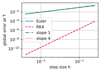
measured slope, Euler: 1.040
measured slope, RK4  : 4.022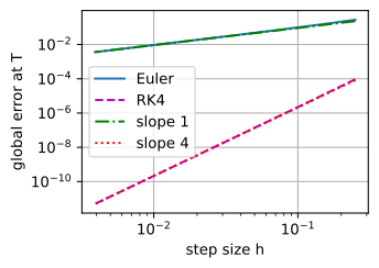
measured slope, Euler: 1.040
measured slope, RK4  : 4.022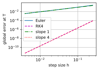
measured slope, Euler: 1.040
measured slope, RK4  : 4.022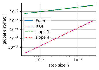
The fitted slopes are within a few percent of the theoretical orders \(1\) and \(4\), and the RK4 curve sits nearly nine decades below Euler at the smallest step (\(3.6 \times 10^{-3}\) versus \(5.0 \times 10^{-12}\)): same trajectory, same horizon, four times the work per step, nearly a billion times the accuracy.
29.1.3.3 Stiffness and Implicit Methods
Order alone does not determine performance. Accuracy measures how closely a numerical path tracks the solution; stability asks whether errors decay or compound into an explosion, and for explicit methods like Euler and RK4, stability puts a hard ceiling on the step size. The phenomenon is already visible in one dimension.
Proposition (stability of Euler on the test equation). On \(\dot{x} = -\lambda x\) with \(\lambda > 0\) (true solution: decay to zero): forward Euler gives \(x_n = (1 - h\lambda)^n x_0\), which decays iff \(|1 - h\lambda| < 1\), i.e.
\[ h < \frac{2}{\lambda} . \]
Backward (implicit) Euler, \(\mathbf{x}_{n+1} = \mathbf{x}_n + h\,\mathbf{f}(\mathbf{x}_{n+1}, t_{n+1})\), gives \(x_n = (1 + h\lambda)^{-n} x_0\), which decays for every \(h > 0\).
Proof. Forward Euler: \(x_{n+1} = x_n - h\lambda x_n = (1 - h\lambda)x_n\); iterate. The factor has magnitude below \(1\) iff \(-1 < 1 - h\lambda < 1\), and the left inequality is the binding one: \(h\lambda < 2\). Backward Euler: \(x_{n+1} = x_n - h\lambda x_{n+1}\), so \(x_{n+1} = x_n / (1 + h\lambda)\), and \(0 < (1 + h\lambda)^{-1} < 1\) for all \(h > 0\). \(\blacksquare\)
Past the threshold, forward Euler amplifies: each step overshoots the origin and has greater magnitude on the other side, producing oscillatory divergence with growth factor \(|1 - h\lambda|\). A method that decays on the test equation for every \(h > 0\) is called A-stable (Dahlquist 1963), and backward Euler is one. (Our \(\lambda\) is real, but the complete stability region is defined in the complex plane. Write the test equation as \(\dot{y} = \lambda y\) with complex \(\lambda\), so that a decaying, rotating mode has \(\operatorname{Re}\lambda < 0\); a method’s stability region is the set of \(z = h\lambda\) for which its update decays, and A-stability proper demands that this region contain the entire left half-plane. Figure 29.1.4 draws the regions; the computation above, \(z = -h\lambda\) with \(\lambda > 0\), is their slice along the negative real axis.) The price of implicitness is that each step defines \(\mathbf{x}_{n+1}\) only implicitly, requiring an equation solve per step, a linear solve when \(\mathbf{f}\) is linear and a few Newton iterations (Section 25.2) otherwise.
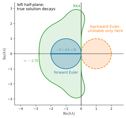
Why tolerate that price? Stiffness. A system is stiff when the step size that stability forces on an explicit method is far smaller than the one accuracy would need. The standard linear source is eigenvalues spread over wildly different scales, say eigenvalues \(-50\) and \(-1\), i.e. decay rates \(\lambda_{\textrm{fast}} = 50\) and \(\lambda_{\textrm{slow}} = 1\). The fast mode decays almost immediately, after which only the slow smooth mode, for which a large step would be perfectly accurate. But forward Euler’s stability constraint \(h < 2/\lambda_{\textrm{fast}}\) is set by the fastest decay rate, including modes that have already decayed and contribute little to the quantity being tracked. The fast mode still governs the explicit method’s stability budget; that mismatch is stiffness. An implicit method removes this particular constraint and lets the step size follow the slower dynamics of interest. The sweep below shows the forward-Euler threshold appear exactly at \(h = 2/\lambda = 0.04\), backward Euler decaying at every step size, and divergence of the two-scale system in the fast component whose exact value had already decayed to \(10^{-22}\).
lam_f = 50.0                                   # the test equation dx/dt = -50 x
T = 1.0
print('forward Euler is stable iff h < 2/lambda =', 2 / lam_f)
print(f'{"h":>8} {"|1-h*lam|":>10} {"forward x(T)":>14} {"backward x(T)":>14}')
for n in [10, 20, 26, 40, 100]:
    h = T / n
    fwd = (1 - h * lam_f) ** n                 # forward Euler after n steps
    bwd = (1 + h * lam_f) ** (-n)              # backward Euler after n steps
    print(f'{h:8.3f} {abs(1 - h * lam_f):10.2f} {fwd:14.2e} {bwd:14.2e}')
print('exact x(T) = e^{-50} =', f'{np.exp(-lam_f * T):.2e}')
A_stiff = np.diag([-50.0, -1.0])               # one fast mode, one slow mode
x_stiff = euler(lambda x: A_stiff @ x, np.array([1.0, 1.0]), T, 20)
print('stiff system, forward Euler with h=0.05 '
      '(the long-dead fast mode explodes):')
print('x(T) =', x_stiff.round(2))
forward Euler is stable iff h < 2/lambda = 0.04
h |1-h*lam| forward x(T) backward x(T)
0.100 4.00 1.05e+06 1.65e-08
0.050 1.50 3.33e+03 1.31e-11
0.038 0.92 1.25e-01 7.73e-13
0.025 0.25 8.27e-25 8.18e-15
0.010 0.50 7.89e-31 2.46e-18
exact x(T) = e^{-50} = 1.93e-22
stiff system, forward Euler with h=0.05 (the long-dead fast mode explodes):
x(T) = [3.32526e+03 3.60000e-01]Note what backward Euler’s unconditional stability does and does not buy: at \(h = 0.1\) it returns \(1.65 \times 10^{-8}\) where the truth is \(1.93 \times 10^{-22}\): stable (it decays, and further steps decay further) but not accurate. Stability prevents the explosion; accuracy may still require a smaller step or a higher-order method. The practical conclusion carries to every learned ODE in Section 29.4: use explicit adaptive solvers by default, and reach for implicit methods when the dynamics are stiff. For a nonlinear or learned field, stiff means that the Jacobian’s eigenvalues along the trajectory are spread over widely different scales.
29.1.3.4 Gradient Descent as Euler Discretization
The same numerical analysis applies to optimization. Infinitesimal descent on a loss \(L\) defines the gradient flow
\[ \dot{\mathbf{x}} = -\nabla L(\mathbf{x}), \]
a vector field whose fixed points are exactly the critical points of \(L\) and along whose trajectories the loss can only fall: \(\tfrac{d}{dt} L(\mathbf{x}(t)) = \nabla L^\top \dot{\mathbf{x}} = -\|\nabla L\|^2 \le 0\). Gradient descent with learning rate \(\eta\) is forward Euler on this flow (\(\mathbf{x}_{k+1} = \mathbf{x}_k - \eta\, \nabla L(\mathbf{x}_k)\) is Equation 29.1.5 with \(h = \eta\)). Solver stability therefore gives the corresponding stability condition for gradient descent. Section 26.1 derived the learning-rate ceiling \(\eta < 2/\lambda_{\max}(H)\) from the quadratic analysis and ran the experiment below; the ODE formulation provides a stability interpretation. Near a minimum with Hessian \(H\) the dynamics linearize, mode by eigenmode, onto the test equation:
\[ \begin{aligned} \dot{\mathbf{x}} = -\nabla L(\mathbf{x}) \;\;&\xrightarrow{\textrm{linearize}}\;\; \dot{\boldsymbol{\delta}} = -H\boldsymbol{\delta} \;\;\xrightarrow{\textrm{Euler}, \, h = \eta}\;\; \boldsymbol{\delta}_{k+1} = (I - \eta H)\,\boldsymbol{\delta}_k \\ &\xrightarrow{\textrm{stability}}\;\; \eta < \frac{2}{\lambda_{\max}(H)} . \end{aligned} \]
The solver bound \(h < 2/\lambda\) is the learning-rate ceiling: a diverging learning rate is a solver instability, and an ill-conditioned Hessian is a stiff gradient flow, with the steep, already-converged curvature directions setting the stability limit under which the shallow directions must then crawl. Polyak’s heavy-ball momentum discretizes the second-order ODE \(m\, \ddot{\mathbf{x}} + \gamma\, \dot{\mathbf{x}} = -\nabla L(\mathbf{x})\) analyzed in Section 26.1. We rerun that section’s experiment on a quadratic with \(\lambda_{\max} = 10\) and compare it with the stiffness sweep: predicted flip at \(\eta = 2/10 = 0.2\).
H = np.diag([10.0, 1.0])                       # curvatures: lambda_max = 10
print('GD on this quadratic is stable iff eta < 2/lambda_max =', 2 / H[0, 0])
print(f'{"eta":>8} {"|1-eta*lam_max|":>16} {"||x|| after 100 GD steps":>25}')
for eta in [0.05, 0.15, 0.19, 0.201, 0.21, 0.25]:
    x = np.array([1.0, 1.0])
    for _ in range(100):
        x = x - eta * (H @ x)                  # gradient descent = forward Euler
    print(f'{eta:8.3f} {abs(1 - eta * H[0, 0]):16.2f} {np.linalg.norm(x):25.2e}')
GD on this quadratic is stable iff eta < 2/lambda_max = 0.2
eta |1-eta*lam_max| ||x|| after 100 GD steps
0.050 0.50 5.92e-03
0.150 0.50 8.75e-08
0.190 0.90 2.66e-05
0.201 1.01 2.70e+00
0.210 1.10 1.38e+04
0.250 1.50 4.07e+17The numerical behavior changes at the predicted threshold. At \(\eta = 0.19\) the fast coordinate contracts by \(|1 - 1.9| = 0.9\) per step and a hundred steps crush the iterate to \(10^{-5}\); at \(\eta = 0.201\) the factor is \(-1.01\) and the same hundred steps have grown it, oscillating in sign, past its starting point; at \(\eta = 0.25\) it has diverged by seventeen orders of magnitude. Meanwhile the slow direction (\(\lambda = 1\)) was converging at every one of these rates. The unstable behavior comes entirely from the loss surface’s stiffest mode.
29.1.4 Neural ODEs and the Adjoint Method
29.1.4.1 Residual Blocks as Euler Steps
A residual update has the same algebraic form as a forward-Euler step.
Proposition (a residual block has the form of an Euler step). The residual update (He et al. 2016)
\[ \mathbf{x}_{l+1} = \mathbf{x}_l + \mathbf{f}_\theta(\mathbf{x}_l) \]
is exactly one forward-Euler step Equation 29.1.5 of the ODE \(\dot{\mathbf{x}} = \mathbf{f}_\theta(\mathbf{x})\) with step size \(h = 1\).
Proof. Set \(h = 1\) and \(\mathbf{f} = \mathbf{f}_\theta\) in Equation 29.1.5; the two updates are the same formula. \(\blacksquare\)
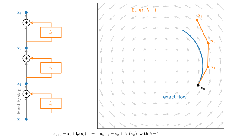
A residual update can therefore be read as one numerical step. A general ResNet may use a different branch \(\mathbf{f}_{\theta_l}\) at every layer; its numerical interpretation is a time-dependent field sampled at the layer times. The interpretation alone gives no invertibility guarantee. For example, \(\dot{x}=-x\) has the bijective exact flow \(e^{-t}x\), whereas one Euler step with \(h=1\) maps every \(x\) to zero.
A continuous-depth limit requires a consistent family of fields and shrinking steps. For the shared field \(\mathbf{x}_{l+1}=\mathbf{x}_l+\tfrac{1}{N}\mathbf{f}_\theta(\mathbf{x}_l)\), Euler convergence implies that the output approaches the exact time-one flow \(\Phi_1(\mathbf{x}_0)\) as \(N\to\infty\), under the regularity assumptions of Section 29.1.3. The limiting model is the Neural ODE (Chen et al. 2018):
\[ \dot{\mathbf{x}} = \mathbf{f}_\theta(\mathbf{x}, t), \qquad \textrm{output} = \mathbf{x}(T) = \mathbf{x}_0 + \int_0^T \mathbf{f}_\theta(\mathbf{x}(t), t)\,dt . \]
The exact Neural ODE map is well-posed and invertible when its field satisfies the existence assumptions in both time directions. A numerical solver approximates that map. Changing Euler to RK4 or an adaptive method leaves the field parameters fixed but changes the computed map, its cost, and its error.
29.1.4.2 Training Through the Solver
The direct training route is discretize, then differentiate: unroll a fixed solver, say \(N\) Euler steps, into the computation graph, compute the loss on \(\mathbf{x}_N\), and apply ordinary backpropagation flow through the unrolled steps. The “network” this builds is equivalent to a ResNet with \(N\) blocks that share the same weights \(\theta\), so ordinary automatic differentiation already trains it.
Consider a task small enough to inspect directly: learn a planar field \(\mathbf{f}_\theta\) (one hidden layer, \(32\) tanh units) whose time-\(1\) flow carries the unit circle onto a shifted, squashed ellipse. We use \(64\) paired points, mean-squared loss on the endpoints, \(10\) unrolled Euler steps of size \(h = 0.1\), and Adam (Section 26.2) as the optimizer. The underlying ODE describes a smooth invertible deformation of \(\mathbb{R}^2\); the ten-step Euler program is its numerical approximation. We supervise only the \(64\) listed points.
theta = np.linspace(0, 2 * np.pi, 64, endpoint=False)
X0_ring = np.stack([np.cos(theta), np.sin(theta)], axis=1)
X1_ring = np.stack([1.5 + 1.2 * np.cos(theta), 0.4 * np.sin(theta)], axis=1)
torch.manual_seed(0)
X, Y = torch.tensor(X0_ring).float(), torch.tensor(X1_ring).float()
net = torch.nn.Sequential(torch.nn.Linear(2, 32), torch.nn.Tanh(),
                          torch.nn.Linear(32, 2))
N, h = 10, 0.1                                 # unrolled Euler: 10 steps to T = 1

def flow(X):
    for _ in range(N):                         # one Euler step = one residual block
        X = X + h * net(X)
    return X

opt = torch.optim.Adam(net.parameters(), lr=0.05)
for it in range(401):
    loss = ((flow(X) - Y) ** 2).mean()
    opt.zero_grad()
    loss.backward()
    opt.step()
    if it % 100 == 0:
        print(f'iter {it:3d}  loss {loss.item():.5f}')
print(f'mean endpoint error: {(flow(X) - Y).norm(dim=1).mean().item():.4f}')
iter 0 loss 1.16972
iter 100 loss 0.00004
iter 200 loss 0.00000
iter 300 loss 0.00000
iter 400 loss 0.00000
mean endpoint error: 0.0011theta = np.linspace(0, 2 * np.pi, 64, endpoint=False)
X0_ring = np.stack([np.cos(theta), np.sin(theta)], axis=1)
X1_ring = np.stack([1.5 + 1.2 * np.cos(theta), 0.4 * np.sin(theta)], axis=1)
tf.random.set_seed(0)
X, Y = tf.constant(X0_ring, tf.float32), tf.constant(X1_ring, tf.float32)
net = tf.keras.Sequential([tf.keras.layers.Dense(32, activation='tanh'),
tf.keras.layers.Dense(2)])
N, h = 10, 0.1 # unrolled Euler: 10 steps to T = 1
def flow(X):
for _ in range(N): # one Euler step = one residual block
X = X + h * net(X)
return X
opt = tf.keras.optimizers.Adam(learning_rate=0.05)
@tf.function
def train_step():
with tf.GradientTape() as tape:
loss = tf.reduce_mean((flow(X) - Y) ** 2)
opt.apply_gradients(zip(tape.gradient(loss, net.trainable_variables),
net.trainable_variables))
return loss
for it in range(401):
loss = train_step()
if it % 100 == 0:
print(f'iter {it:3d} loss {float(loss):.5f}')
err = tf.reduce_mean(tf.norm(flow(X) - Y, axis=1))
print(f'mean endpoint error: {float(err):.4f}')iter 0 loss 1.36651
iter 100 loss 0.00007
iter 200 loss 0.00002
iter 300 loss 0.00000
iter 400 loss 0.00000
mean endpoint error: 0.0015theta = np.linspace(0, 2 * np.pi, 64, endpoint=False)
X0_ring = np.stack([np.cos(theta), np.sin(theta)], axis=1)
X1_ring = np.stack([1.5 + 1.2 * np.cos(theta), 0.4 * np.sin(theta)], axis=1)
k1, k2 = jax.random.split(jax.random.PRNGKey(0))
params = {'W1': 0.25 * jax.random.normal(k1, (2, 32)), 'b1': jnp.zeros(32),
'W2': 0.25 * jax.random.normal(k2, (32, 2)), 'b2': jnp.zeros(2)}
X, Y = jnp.array(X0_ring), jnp.array(X1_ring)
N, h = 10, 0.1 # unrolled Euler: 10 steps to T = 1
def flow(params, X):
field = lambda X: (jnp.tanh(X @ params['W1'] + params['b1'])
@ params['W2'] + params['b2'])
return jax.lax.fori_loop(0, N, lambda i, X: X + h * field(X), X)
loss_fn = lambda params: ((flow(params, X) - Y) ** 2).mean()
@jax.jit
def adam_step(params, m, v, it): # hand-rolled Adam, lr = 0.05
loss, g = jax.value_and_grad(loss_fn)(params)
m = jax.tree.map(lambda m, g: 0.9 * m + 0.1 * g, m, g)
v = jax.tree.map(lambda v, g: 0.999 * v + 0.001 * g * g, v, g)
upd = lambda p, m, v: p - 0.05 * (m / (1 - 0.9 ** it)) / (
jnp.sqrt(v / (1 - 0.999 ** it)) + 1e-8)
return jax.tree.map(upd, params, m, v), m, v, loss
m = jax.tree.map(jnp.zeros_like, params)
v = jax.tree.map(jnp.zeros_like, params)
for it in range(1, 402):
params, m, v, loss = adam_step(params, m, v, jnp.float32(it))
if it % 100 == 1:
print(f'iter {it - 1:3d} loss {float(loss):.5f}')
err = jnp.linalg.norm(flow(params, X) - Y, axis=1).mean()
print(f'mean endpoint error: {float(err):.4f}')iter 0 loss 1.18094
iter 100 loss 0.00011
iter 200 loss 0.00002
iter 300 loss 0.00001
iter 400 loss 0.00000
mean endpoint error: 0.0021theta = np.linspace(0, 2 * np.pi, 64, endpoint=False)
X0_ring = np.stack([np.cos(theta), np.sin(theta)], axis=1)
X1_ring = np.stack([1.5 + 1.2 * np.cos(theta), 0.4 * np.sin(theta)], axis=1)
npx.random.seed(0)
X, Y = mnp.array(X0_ring), mnp.array(X1_ring)
net = nn.Sequential()
net.add(nn.Dense(32, activation='tanh'), nn.Dense(2))
net.initialize(init.Xavier())
N, h = 10, 0.1 # unrolled Euler: 10 steps to T = 1
def flow(X):
for _ in range(N): # one Euler step = one residual block
X = X + h * net(X)
return X
trainer = gluon.Trainer(net.collect_params(), 'adam', {'learning_rate': 0.05})
for it in range(401):
with autograd.record():
loss = ((flow(X) - Y) ** 2).mean()
loss.backward()
trainer.step(1)
if it % 100 == 0:
print(f'iter {it:3d} loss {float(loss):.5f}')
err = mnp.sqrt(((flow(X) - Y) ** 2).sum(axis=1)).mean()
print(f'mean endpoint error: {float(err):.4f}')iter 0 loss 1.27961[18:54:29] /home/smola/mxnet/src/base.cc:48: GPU context requested, but no GPUs found.iter 100 loss 0.00003
iter 200 loss 0.00001
iter 300 loss 0.00000
iter 400 loss 0.00000
mean endpoint error: 0.0013A few hundred full-batch Adam iterations drive the loss to \(\sim 10^{-5}\) and the mean endpoint error to \(\sim 10^{-3}\): one tiny vector field, integrated by ten shared-weight residual updates, learns the prescribed endpoints. Integrating the learned continuous field backward approximates its inverse flow. The forward and backward numerical maps agree only up to solver error; the ten-step Euler map itself is not guaranteed to be invertible.
29.1.4.3 The Adjoint Method: Backpropagation in Continuous Time
Differentiating through the unrolled solver computes the exact gradient of the discretized program, but ordinarily stores its intermediate states. The continuous adjoint method instead differentiates the exact ODE problem and integrates a second ODE backward in time. With recomputation it can reduce stored solver states, at the cost of additional evaluations and possible numerical mismatch. Its central object is the adjoint state \(\mathbf{a}(t) = \partial L / \partial \mathbf{x}(t)\) (“how would the loss change if the trajectory were nudged at time \(t\)?”), the continuous analogue of the backprop delta of Section 25.3.
Proposition (the adjoint equations). Let \(\mathbf{f}\) be continuously differentiable in \(\mathbf{x}\) and \(\theta\), let \(\mathbf{x}(t)\) solve \(\dot{\mathbf{x}} = \mathbf{f}(\mathbf{x}, \theta, t)\) on \([0, T]\) from fixed \(\mathbf{x}(0)\), and let \(L = \ell(\mathbf{x}(T))\) be a differentiable loss on the endpoint. Then the adjoint state satisfies the linear ODE
\[ \dot{\mathbf{a}}(t) = -\left(\frac{\partial \mathbf{f}}{\partial \mathbf{x}}\right)^{\!\top}\! \mathbf{a}(t), \qquad \mathbf{a}(T) = \nabla \ell(\mathbf{x}(T)), \tag{29.1.7}\]
integrated backward from \(T\), and the parameter gradient is the integral
\[ \frac{\partial L}{\partial \theta} = \int_0^T \left(\frac{\partial \mathbf{f}}{\partial \theta}\right)^{\!\top}\! \mathbf{a}(t)\, dt, \tag{29.1.8}\]
with both partial derivatives evaluated along the trajectory \((\mathbf{x}(t), \theta, t)\) (Chen et al. 2018).
Proof (variational). Perturb the parameters by an infinitesimal \(\delta\theta\) and analyze the resulting trajectory perturbation. Because \(\mathbf{f}\) is \(C^1\), the flow is differentiable in \(\theta\) and the first-order expansion below is rigorous: the perturbation \(\delta\mathbf{x}(t)\) obeys the linearization of the dynamics (differentiate the ODE in \(\theta\) and use the chain rule):
\[ \delta\dot{\mathbf{x}} = \frac{\partial \mathbf{f}}{\partial \mathbf{x}}\,\delta\mathbf{x} + \frac{\partial \mathbf{f}}{\partial \theta}\,\delta\theta, \qquad \delta\mathbf{x}(0) = \mathbf{0}. \]
Define \(\mathbf{a}(t)\) by the backward ODE Equation 29.1.7 and examine the pairing \(\mathbf{a}^\top \delta\mathbf{x}\) evolve; the derivative telescopes by design:
\[ \frac{d}{dt}\left(\mathbf{a}^\top \delta\mathbf{x}\right) = \dot{\mathbf{a}}^\top \delta\mathbf{x} + \mathbf{a}^\top \delta\dot{\mathbf{x}} = -\mathbf{a}^\top \frac{\partial \mathbf{f}}{\partial \mathbf{x}}\,\delta\mathbf{x} + \mathbf{a}^\top \frac{\partial \mathbf{f}}{\partial \mathbf{x}}\,\delta\mathbf{x} + \mathbf{a}^\top \frac{\partial \mathbf{f}}{\partial \theta}\,\delta\theta = \mathbf{a}^\top \frac{\partial \mathbf{f}}{\partial \theta}\,\delta\theta . \]
The state-coupling terms cancel exactly; that cancellation is why the adjoint ODE has the form it has. Integrate from \(0\) to \(T\), using \(\delta\mathbf{x}(0) = \mathbf{0}\) on the left endpoint:
\[ \mathbf{a}(T)^\top \delta\mathbf{x}(T) = \int_0^T \mathbf{a}(t)^\top \frac{\partial \mathbf{f}}{\partial \theta}\, dt \;\delta\theta . \]
The left side is \(\nabla\ell(\mathbf{x}(T))^\top \delta\mathbf{x}(T) = \delta L\), the first-order change of the loss; the right side is linear in \(\delta\theta\) with coefficient Equation 29.1.8. (The same telescoping, stopped at an intermediate time \(s\), shows \(\delta L = \mathbf{a}(s)^\top \delta\mathbf{x}(s)\) for a nudge injected at time \(s\), so the solution of Equation 29.1.7 really is \(\partial L/\partial \mathbf{x}(s)\), earning its name.) \(\blacksquare\)
One caveat connects back to Section 29.1.1.3: the existence theorem tolerates ReLU fields, but the adjoint equations as stated need a \(C^1\) field. A ReLU field is differentiable only piecewise; in practice autograd differentiates the unrolled solver piece by piece, and smooth activations (tanh, GELU) remove the issue entirely.
Each backward-ODE step computes \(-\mathbf{a}^\top \partial\mathbf{f}/\partial\mathbf{x}\) is a vector–Jacobian product, the very primitive that reverse-mode AD is made of (Section 25.3). Discretize Equation 29.1.7 with the same Euler scheme as the forward pass and the result is the backpropagation recursion through the unrolled network: backprop is the discrete adjoint method, a lineage that runs from optimal control (Pontryagin et al. 1962) straight to the backward pass of every deep-learning framework. The continuous formulation offers another implementation: instead of storing the forward states for the VJPs, one may re-integrate \(\mathbf{x}(t)\) backward alongside \(\mathbf{a}(t)\), making constant memory in the number of stored trajectory checkpoints in an idealized implementation, at the cost of extra compute and of numerical drift when the reversed dynamics are unstable (a strongly contracting forward flow is, run backward, strongly expanding; in that regime checkpointing or plain unrolling is the sturdier choice). The literature names the two routes discretize-then-optimize (differentiate the unrolled solver, exact for the executed program) versus optimize-then-discretize (discretize the continuous adjoint, using less trajectory storage but generally producing only an approximation to the gradient of the discrete forward program) (Kidger 2022); Exercise 7 probes exactly this fault line.
The preceding identities can be checked on the linear ODE \(\dot{\mathbf{x}} = A\mathbf{x}\), where every ingredient has a closed form: the trajectory is \(e^{At}\mathbf{x}_0\), the adjoint of \(L = \tfrac12\|\mathbf{x}(T)\|^2\) is \(\mathbf{a}(t) = e^{A^\top (T-t)}\,\mathbf{x}(T)\) (the adjoint ODE \(\dot{\mathbf{a}} = -A^\top\mathbf{a}\) run backward), and with \(\theta\) the entries of \(A\) itself, \(\partial\mathbf{f}/\partial A\) turns Equation 29.1.8 into \(\partial L/\partial A = \int_0^T \mathbf{a}(t)\,\mathbf{x}(t)^\top dt\). The cell computes the gradient three ways: hand-written reverse mode through the unrolled Euler solver (the discrete adjoint: exactly what reverse-mode autograd builds, written out in six lines), central finite differences on the same unrolled program, and the continuous adjoint integral by quadrature.
def expm_eig(B, s):
    """e^{Bs} via the eigendecomposition formula."""
    mu, W = np.linalg.eig(B)
    return (W @ np.diag(np.exp(mu * s)) @ np.linalg.inv(W)).real

def loss_and_grad_unrolled(A, x0, T, n):
    """L = ||x_n||^2 / 2 through n unrolled Euler steps; dL/dA by hand-written
    reverse mode -- the discrete adjoint."""
    h, xs = T / n, [x0]
    for k in range(n):
        xs.append(xs[-1] + h * (A @ xs[-1]))   # forward sweep, tape the states
    a, gA = xs[-1].copy(), np.zeros_like(A)    # a_n = dL/dx_n = x_n
    for k in range(n - 1, -1, -1):             # backward sweep: one VJP per step
        gA += h * np.outer(a, xs[k])           # dL/dA  +=  h a_{k+1} x_k^T
        a = a + h * (A.T @ a)                  # a_k = (I + hA)^T a_{k+1}
    return 0.5 * xs[-1] @ xs[-1], gA

T, n = 2.0, 1000
L, g_disc = loss_and_grad_unrolled(A, x0, T, n)
g_fd = np.zeros_like(A)                        # central finite differences
for i in range(2):
    for j in range(2):
        E = np.zeros_like(A); E[i, j] = 1e-5
        g_fd[i, j] = (loss_and_grad_unrolled(A + E, x0, T, n)[0]
                      - loss_and_grad_unrolled(A - E, x0, T, n)[0]) / 2e-5
print('discrete adjoint vs finite differences:', f'{np.abs(g_disc - g_fd).max():.1e}')

m = 2000                                       # continuous adjoint, trapezoid rule
ts = np.linspace(0.0, T, m + 1)
xT = expm_eig(A, T) @ x0
F = np.stack([np.outer(expm_eig(A.T, T - s) @ xT, expm_eig(A, s) @ x0)
              for s in ts])
g_cont = (T / m) * (F[1:-1].sum(axis=0) + 0.5 * (F[0] + F[-1]))
for n_steps in [100, 1000, 10000]:
    gap = np.abs(loss_and_grad_unrolled(A, x0, T, n_steps)[1] - g_cont).max()
    print(f'n = {n_steps:6d} Euler steps: |discrete - continuous adjoint| = {gap:.1e}')
discrete adjoint vs finite differences: 1.2e-10
n = 100 Euler steps: |discrete - continuous adjoint| = 2.9e-02
n = 1000 Euler steps: |discrete - continuous adjoint| = 2.8e-03
n = 10000 Euler steps: |discrete - continuous adjoint| = 2.8e-04The discrete adjoint matches finite differences to \(10^{-10}\) (it is the exact gradient of the unrolled program), and as the solver is refined the discrete gradient converges to the continuous adjoint integral at exactly the solver’s order, \(O(h)\): ten times the steps, one-tenth the gap. Backprop through a solver and the adjoint method are one algorithm, seen at two resolutions.
29.1.5 Continuous Normalizing Flows
29.1.5.1 The Instantaneous Change of Variables
Pushing samples through a Neural ODE defines a generative model. Maximum- likelihood training additionally requires the change in density along the flow. The discrete answer we know from Section 27.1: for an invertible map \(\mathbf{g}\) with Jacobian \(J_{\mathbf{g}}\),
\[ \log p_{\textrm{out}}(\mathbf{g}(\mathbf{x})) = \log p_{\textrm{in}}(\mathbf{x}) - \log \left|\det J_{\mathbf{g}}(\mathbf{x})\right| , \]
and a normalizing flow built from \(K\) layers evaluates one log-determinant per layer. The \(O(d^3)\) determinant is the reason discrete flows constrain their layers to triangular or low-rank Jacobians. In continuous time the formula simplifies: over one infinitesimal step the flow map is near-identity, and the determinant of a near-identity matrix is governed by the trace.
Lemma. For any square matrix \(J\), \(\det(I + hJ) = 1 + h \operatorname{tr} J + O(h^2)\).
Proof. In the Leibniz expansion of the determinant, any permutation other than the identity uses at least two off-diagonal entries, each of size \(O(h)\), so contributes \(O(h^2)\). The identity permutation contributes \(\prod_i (1 + h J_{ii}) = 1 + h \sum_i J_{ii} + O(h^2)\). \(\blacksquare\)
Proposition (instantaneous change of variables). Let \(\dot{\mathbf{x}} = \mathbf{f}(\mathbf{x}, t)\) with \(\mathbf{f}\) continuously differentiable and \(\mathbf{x}(0) \sim p_0\) for a differentiable density \(p_0\), and let \(p_t\) denote the density of \(\mathbf{x}(t)\), which then exists and is differentiable along trajectories. Then along each trajectory (Chen et al. 2018)
\[ \frac{d}{dt} \log p_t(\mathbf{x}(t)) = -\operatorname{tr}\!\left(\frac{\partial \mathbf{f}}{\partial \mathbf{x}}\right)\!(\mathbf{x}(t), t). \tag{29.1.9}\]
Proof. Over a short interval the flow advances by the near-identity map \(\Phi_h(\mathbf{x}) = \mathbf{x} + h\,\mathbf{f}(\mathbf{x}, t) + O(h^2)\), whose Jacobian is \(I + h J + O(h^2)\) with \(J = \partial\mathbf{f}/\partial\mathbf{x}\). Apply the discrete change-of-variables formula to this one map and expand with the Lemma, which tolerates the perturbed argument: replacing \(J\) by \(J + O(h)\) changes \(\det(I + hJ)\) only at order \(h^2\). Thus:
\[ \log p_{t+h}(\mathbf{x}(t+h)) = \log p_t(\mathbf{x}(t)) - \log\det\!\left(I + hJ + O(h^2)\right) = \log p_t(\mathbf{x}(t)) - h \operatorname{tr} J + O(h^2), \]
using \(\log(1 + u) = u + O(u^2)\) (for small \(h\) the determinant is positive, so the absolute value is moot). Subtract, divide by \(h\), and let \(h \to 0\). \(\blacksquare\)
The trace of the Jacobian is the divergence of the field: the local expansion rate of volume. Where the field spreads (\(\operatorname{tr} J > 0\)), the cloud of samples dilutes and the log-density along each trajectory falls; where it compresses, probability concentrates. Integrating Equation 29.1.9 along the trajectory turns the per-layer log-det sum of a discrete flow into a trace integral:
\[ \log p_T(\mathbf{x}(T)) = \log p_0(\mathbf{x}(0)) - \int_0^T \operatorname{tr}\!\left(\frac{\partial \mathbf{f}}{\partial \mathbf{x}}\right) dt . \tag{29.1.10}\]
This yields the continuous normalizing flow (CNF). Augment the state with its log-density and integrate \((\mathbf{x}, \log p)\) together. Under exact integration, this gives the likelihood for an unconstrained architecture without requiring triangular Jacobians.
29.1.5.2 The Hutchinson Trace Estimator
Directly computing \(\operatorname{tr}(\partial\mathbf{f}/\partial\mathbf{x})\) requires all \(d\) diagonal entries of the Jacobian, or \(d\) derivative passes. Hutchinson’s identity provides an unbiased stochastic estimator (Hutchinson 1989).
Proposition (Hutchinson estimator). For any matrix \(M \in \mathbb{R}^{d \times d}\) and any random \(\boldsymbol{\epsilon} \in \mathbb{R}^d\) with \(\mathbb{E}[\boldsymbol{\epsilon}] = \mathbf{0}\) and \(\mathbb{E}[\boldsymbol{\epsilon}\boldsymbol{\epsilon}^\top] = I\) (Gaussian or Rademacher, i.e. uniform \(\pm 1\) entries),
\[ \operatorname{tr}(M) = \mathbb{E}\!\left[\boldsymbol{\epsilon}^\top M \boldsymbol{\epsilon}\right]. \tag{29.1.11}\]
Proof. \(\mathbb{E}[\boldsymbol{\epsilon}^\top M \boldsymbol{\epsilon}] = \mathbb{E}[\operatorname{tr}(M \boldsymbol{\epsilon}\boldsymbol{\epsilon}^\top)] = \operatorname{tr}(M\, \mathbb{E}[\boldsymbol{\epsilon}\boldsymbol{\epsilon}^\top]) = \operatorname{tr}(M)\), using the cyclic property of the trace and its linearity (which lets it commute with the expectation). \(\blacksquare\)
The point is what the estimator touches: \(\boldsymbol{\epsilon}^\top J\) is a single vector–Jacobian product followed by a dot product: one reverse-mode pass through \(\mathbf{f}\) with cost comparable to one evaluation/backward pass, and no full Jacobian is ever materialized (Section 25.3). The resulting stochastic likelihood estimate requires one additional backward pass, as in FFJORD (Grathwohl et al. 2019).
For a linear field, the result can be checked directly: \(\dot{\mathbf{x}} = A\mathbf{x}\) has constant Jacobian \(A\), so Equation 29.1.10 says the log-density along every trajectory falls at the constant rate \(\operatorname{tr}(A)\): \(\log p_t(\mathbf{x}(t)) = \log p_0(\mathbf{x}_0) - t \operatorname{tr}(A)\). The cell flows standard-normal samples through the spiral field and compares the two answers, since the exact time-\(t\) density is the Gaussian \(\mathcal{N}(\mathbf{0},\, e^{At} e^{A^\top t})\), computable in closed form. Then it verifies the Hutchinson estimator on a random \(6 \times 6\) matrix.
rng = np.random.default_rng(0)
t = 1.5
X0s = rng.standard_normal((4, 2))              # four samples from p_0 = N(0, I)
Et = expm_eig(A, t)
Xts = X0s @ Et.T                               # flow each sample to time t
Sig = Et @ Et.T                                # x(t) ~ N(0, E_t E_t^T)
logp0 = -0.5 * (X0s ** 2).sum(axis=1) - np.log(2 * np.pi)
logpt = (-0.5 * np.einsum('ki,ij,kj->k', Xts, np.linalg.inv(Sig), Xts)
         - 0.5 * np.log(np.linalg.det(Sig)) - np.log(2 * np.pi))
print('log p_t(x(t)), Gaussian formula  :', logpt.round(6))
print('log p_0(x_0) - t tr(A), our rule :', (logp0 - t * np.trace(A)).round(6))

J = rng.standard_normal((6, 6))                # Hutchinson on a bigger matrix
eps = rng.choice([-1.0, 1.0], size=(100000, 6))
est = np.einsum('ki,ij,kj->k', eps, J, eps)
print(f'Hutchinson: tr(J) = {np.trace(J):.4f},  estimate = {est.mean():.4f}'
      f' +- {est.std() / np.sqrt(len(est)):.4f}')
log p_t(x(t)), Gaussian formula : [-0.354507 -0.54845 -0.546723 -1.636566]
log p_0(x_0) - t tr(A), our rule : [-0.354507 -0.54845 -0.546723 -1.636566]
Hutchinson: tr(J) = -1.7535, estimate = -1.7554 +- 0.0173The two log-density computations agree digit for digit (the trace integral equals the log-det-Jacobian evaluated through the trace integral), and the Hutchinson estimate brackets the true trace within its standard error. Finally, Equation 29.1.9 is the trajectory-wise form of the continuity equation governing how a whole density field is transported; Section 29.3 starts there and turns a diffusion’s noisy paths into a deterministic probability-flow ODE integrated by exactly the solvers of this section.
29.1.6 Summary
- An ODE \(\dot{\mathbf{x}} = \mathbf{f}(\mathbf{x}, t)\) is a velocity field; a solution is everywhere tangent to it, and the flow map \(\Phi_t\) moves all of space at once, composing as \(\Phi_{t+s} = \Phi_t \circ \Phi_s\).
- Picard–Lindelöf: a globally Lipschitz field has exactly one trajectory through each point for every finite time (the Picard integral operator is a contraction). Existence and uniqueness in both time directions make its flow maps bijections, the well-posedness behind invertible generative flows. Without Lipschitz, uniqueness fails (\(\dot{x} = \sqrt{|x|}\), a fan of solutions); without a growth bound, solutions can blow up in finite time (\(\dot{x} = x^2\)).
- Linear systems are solved by the matrix exponential \(e^{At} = \sum_k (At)^k/k!\). If \(A\) is diagonalizable, this becomes \(V e^{\Lambda t}V^{-1}\) and separates the eigendirections. Eigenvalue real parts determine asymptotic modal growth, while nonnormal matrices can also exhibit transient growth. Jacobian eigenvalues classify a nonlinear fixed point directly only in the hyperbolic case.
- Explicit solvers have global error \(O(h^p)\): forward Euler has order \(1\) (local \(O(h^2)\) errors, \(T/h\) of them, times an \(e^{LT}\) stability factor), RK4 order \(4\); both slopes are measurable on a log–log plot. Stiffness: forward Euler is stable on \(\dot{x} = -\lambda x\) only for \(h < 2/\lambda\), so a rapidly decaying mode can dictate the step; implicit (backward) Euler is stable for every \(h\), at the price of solving an equation per step, but a stable large step need not be accurate.
- Gradient descent is forward Euler on the gradient flow \(\dot{\mathbf{x}} = -\nabla L\). For a positive-definite quadratic, or locally near such a minimum, the stability bound is \(\eta < 2/\lambda_{\max}(H)\) and ill-conditioning produces the same two-scale restriction as stiffness. Momentum discretizes the heavy-ball ODE \(m\ddot{\mathbf{x}} + \gamma\dot{\mathbf{x}} = -\nabla L\).
- A residual block has the algebraic form of an Euler step. A consistent family with shrinking step size can converge to a Neural ODE; a finite residual stack need not inherit the exact flow’s invertibility. Backpropagation through the solver is the discrete adjoint and gives the discretized program’s exact gradient. The continuous adjoint differentiates the ODE problem and trades saved states for recomputation, tolerance error, and possible reverse-time instability.
- Densities transported by a flow obey the instantaneous change of variables \(\tfrac{d}{dt}\log p_t = -\operatorname{tr}(\partial\mathbf{f}/\partial\mathbf{x})\): the log-det-Jacobian becomes a trace integral, estimated unbiasedly by Hutchinson’s estimator \(\boldsymbol{\epsilon}^\top J \boldsymbol{\epsilon}\) at the cost of one VJP per stochastic trace sample: the mathematics of continuous normalizing flows.
29.1.7 Exercises
- Verify by differentiation that \(\mathbf{x}(t) = e^{-t}\mathbf{x}_0\) solves \(\dot{\mathbf{x}} = -\mathbf{x}\), and that trajectories of the rotational field \(\dot{\mathbf{x}} = \left(\begin{smallmatrix}0&-1\\1&0\end{smallmatrix}\right)\mathbf{x}\) keep \(\|\mathbf{x}(t)\|\) constant. Write the integral form Equation 29.1.2 for \(\dot{x} = t\) and evaluate it.
- Show that a linear field \(\mathbf{f}(\mathbf{x}) = A\mathbf{x}\) is Lipschitz with constant \(\|A\|\) (the operator norm). Then construct a solution of \(\dot{x} = \sqrt{|x|}\), \(x(0) = 0\) that waits at the origin until time \(c\) before leaving, verify it solves the ODE at every \(t\), and identify exactly where the Lipschitz hypothesis fails. Finally, compute the blow-up time of \(\dot{x} = x^2\), \(x(0) = x_0 > 0\), and explain why Picard–Lindelöf only promises a local solution here.
- From the series Equation 29.1.3, show that \(e^{At}\) commutes with \(A\) and that \(e^{A(t+s)} = e^{At}e^{As}\). Then classify the phase portraits of \(\left(\begin{smallmatrix}-2&0\\0&-1\end{smallmatrix}\right)\), \(\left(\begin{smallmatrix}1&0\\0&-1\end{smallmatrix}\right)\), and \(\left(\begin{smallmatrix}0&-2\\2&0\end{smallmatrix}\right)\) using the stability dictionary.
- Derive Euler’s local truncation error \(O(h^2)\) from Taylor’s theorem with remainder, and rehearse the accumulation argument that turns it into a global \(O(h)\). Then show that the midpoint method’s update matches the true Taylor expansion through \(h^2\) in the vector case, where the scalar product \(f'f\) becomes the Jacobian–vector product \((\partial\mathbf{f}/\partial\mathbf{x})\mathbf{f}\).
- Re-derive the forward-Euler stability bound \(h < 2/\lambda\) and backward Euler’s unconditional stability. For the stiff matrix \(A = \mathrm{diag}(-100, -1)\): what step size does forward Euler need for stability, how many steps to reach \(T = 5\), and how do both change if the fast eigenvalue moves to \(-10^4\)? For nonlinear \(\mathbf{f}\), write the equation one backward-Euler step must solve and the Newton iteration you would use.
- A residual block computes \(\mathbf{x}_{l+1} = \mathbf{x}_l + \mathbf{f}_\theta(\mathbf{x}_l)\). Identify the implied step size; explain what halving the solver step while doubling the step count corresponds to architecturally; and use Section 29.1.1.3 to argue that the time-\(T\) flow of a Lipschitz \(\mathbf{f}_\theta\) is invertible; then explain why a plain (non-residual) layer \(\mathbf{x} \mapsto \sigma(W\mathbf{x})\) has no such guarantee.
- Re-derive the adjoint equations Equation 29.1.7 and Equation 29.1.8 from the variational argument without looking. Show that one Euler step of the adjoint ODE is exactly one vector–Jacobian product, and that discretizing the adjoint ODE with Euler reproduces the backpropagation recursion of the
#odes-solvers-adjoint-checkcell. When the forward dynamics contract strongly (all \(\operatorname{Re}\lambda \ll 0\)), what goes wrong with reconstructing \(\mathbf{x}(t)\) by integrating backward, and why does the \(O(1)\)-memory adjoint suffer where unrolled backprop does not? - Derive the instantaneous change of variables Equation 29.1.9 from the discrete log-det formula as \(h \to 0\), and check that for a single linear “layer” \(\Phi_t = e^{At}\) it reproduces \(-\log|\det e^{At}| = -t\operatorname{tr}(A)\) (use \(\det e^{At} = e^{t \operatorname{tr} A}\), e.g. via Equation 29.1.4). Prove the Hutchinson estimator Equation 29.1.11 is unbiased, compute its variance for Rademacher probes (express it in terms of the off-diagonal entries of \(M + M^\top\)), and explain why estimating the trace costs one VJP while the determinant has no comparably cheap unbiased estimator.