%matplotlib inline
from d2l import torch as d2l
import time
import torch
from torch import nn
from torch.nn import functional as F11.4 Encoders, Decoders, and Cross-Attention
The GPT of Section 11.2 uses a causal mask in addition to stacked transformer blocks. This mask supports next-token prediction, but restricts each representation to preceding context. In this section, the attention mask and the sources of queries, keys, and values become design choices. Removing it gives an encoder, which reads in both directions and produces contextual representations. Joining a masked stack to an unmasked one through the cross-attention of Section 10.3 gives the encoder–decoder that transformers started as (Vaswani et al. 2017). We build both from the same d2l.TransformerBlock, examine whether a learned cross-attention map reproduces a known alignment, and then consider learned queries that do not come from an input sequence. These queries provide an interface between fixed-size computation and variable-size data, as used in Perceiver-style and vision–language models.
%matplotlib inline
from d2l import jax as d2l
from flax import nnx
import jax
from jax import numpy as jnp
import optax
import time
11.4.1 Encoder, Decoder, and Encoder–Decoder Architectures
A transformer block maps a sequence of \(d\)-dimensional vectors to a sequence of the same shape, and it leaves two questions open: which positions may attend to which, and where the keys and values come from. Three common wirings answer these questions, and Figure 11.4.1 draws them in the convention we will use for every attention map in this section — queries down the rows, keys along the columns.
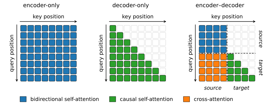
Encoder-only. Drop the mask. Every token attends to every other, so each output vector summarizes the whole input as seen from its position. Such a model does not directly implement the left-to-right autoregressive factorization: with the future visible, next-token prediction is a copying exercise (though masked models can still be decoded by iterative re-masking, the idea text diffusion models develop). But it is the strongest way to represent an input, and one representation per token is exactly what classification, retrieval, and tagging consume. BERT is this wiring pretrained on text (Devlin et al. 2018); the vision transformer of Section 11.5 is the same wiring over image patches.
Decoder-only. Keep the causal mask everywhere: the GPT of Section 11.2, in two sentences. Each token predicts its successor, generation is the training objective run forward, and one stack serves both understanding and production. We do not rebuild it here; it appears in Figure 11.4.1 as the pattern the other two are measured against.
Encoder–decoder. The original transformer (Vaswani et al. 2017) combines the two: a bidirectional encoder reads the source sequence, and a causal decoder generates the target while cross-attending into the encoder’s output — queries from the target stream, keys and values from the source, the second wiring of Section 10.3. The pattern in Figure 11.4.1 shows the division: a full square for the source, a full rectangle for target-to-source cross-attention, a triangle for the target’s own past. Machine translation was the founding application; T5 pretrained the architecture on span reconstruction and recast a broad family of tasks as text-to-text (Raffel et al. 2020), BART on denoising corrupted text (Lewis et al. 2019).
The rest of this section builds the two wirings that Section 11.2 did not, in order.
11.4.2 Bidirectional Context for Masked-Token Prediction
11.4.2.1 A Bidirectional Encoder in a Dozen Lines
The encoder differs from the CharLM of Section 11.1 by a single argument: we pass no valid_lens, so nothing is masked. Positions are still the model’s job, since attention is permutation equivariant (Section 10.4), so a learned position table stays.
class TransformerEncoder(nn.Module):
    """Bidirectional encoder: embeddings plus unmasked pre-norm blocks."""
    def __init__(self, vocab_size, num_hiddens=128, num_heads=4, num_blks=4,
                 max_len=64):
        super().__init__()
        self.token_emb = nn.Embedding(vocab_size, num_hiddens)
        self.pos_emb = nn.Embedding(max_len, num_hiddens)
        for emb in (self.token_emb, self.pos_emb):
            nn.init.normal_(emb.weight, std=0.02)
        self.blks = nn.ModuleList([
            d2l.TransformerBlock(num_hiddens, num_heads)
            for _ in range(num_blks)])
        self.norm = nn.RMSNorm(num_hiddens)

    def forward(self, X):
        H = self.token_emb(X) + self.pos_emb(
            torch.arange(X.shape[1], device=X.device))
        for blk in self.blks:
            H = blk(H)  # no valid_lens: every token attends everywhere
        return self.norm(H)
class TransformerEncoder(nnx.Module):
"""Bidirectional encoder: embeddings plus unmasked pre-norm blocks."""
def __init__(self, vocab_size, num_hiddens=128, num_heads=4, num_blks=4,
max_len=64, rngs=None):
rngs = nnx.Rngs(0) if rngs is None else rngs
init = nnx.initializers.normal(0.02)
self.token_emb = nnx.Embed(vocab_size, num_hiddens,
embedding_init=init, rngs=rngs)
self.pos_emb = nnx.Embed(max_len, num_hiddens, embedding_init=init,
rngs=rngs)
self.blks = nnx.List([
d2l.TransformerBlock(num_hiddens, num_heads, rngs=rngs)
for _ in range(num_blks)])
self.norm = nnx.RMSNorm(num_hiddens, rngs=rngs)
def __call__(self, X):
H = self.token_emb(X) + self.pos_emb(jnp.arange(X.shape[1]))
for blk in self.blks:
H = blk(H) # no valid_lens: every token attends everywhere
return self.norm(H)11.4.2.2 The Masked-Token Objective
What should this model train on? Not next-token prediction: with the future visible, position \(t\) can read token \(t+1\) directly, and the loss collapses without teaching anything. The objective must hide what it asks for. Masked language modeling (Devlin et al. 2018) replaces a random subset of tokens with a special <mask> symbol and asks the model to reconstruct them from everything that remains:
\[ \max \; \sum_{t \in \mathcal{M}} \log p\left(x_t \mid \mathbf{x}_{\setminus \mathcal{M}}\right), \tag{11.4.1}\]
where \(\mathcal{M}\) is the masked set. Prediction at a masked position draws on context from both sides, the capability provided by removing the causal mask. We train the recipe in miniature on the character-level Time Machine corpus of Section 8.2, masking 15% of characters per window and giving <mask> one extra embedding row; the tied output head is the same trick as in Section 11.1.
data = d2l.TimeMachine(batch_size=64, num_steps=64, tokenization='char',
                       num_train=100000, num_val=3000)
MASK = len(data.vocab)  # id of the extra <mask> embedding row

def mask_tokens(X, p=0.15):
    mask = torch.rand(X.shape, device=X.device) < p
    return torch.where(mask, torch.full_like(X, MASK), X), mask

torch.manual_seed(0)
device = d2l.try_gpu()
model = TransformerEncoder(len(data.vocab) + 1).to(device)
optimizer = torch.optim.AdamW(model.parameters(), lr=1e-3,
                              weight_decay=0.0)
losses, step = [], 0
while step < 2000:
    for X, _ in data.train_dataloader():
        X = X.to(device)
        Xm, mask = mask_tokens(X)
        logits = F.linear(model(Xm), model.token_emb.weight)
        loss = F.cross_entropy(logits[mask], X[mask])
        optimizer.zero_grad()
        loss.backward()
        optimizer.step()
        losses.append(loss.item())
        step += 1
        if step >= 2000:
            break
print('masked loss at step 500/1000/2000: ' + '/'.join(
    f'{sum(losses[k-50:k]) / 50:.2f}' for k in (500, 1000, 2000)))
masked loss at step 500/1000/2000: 1.92/1.35/1.08data = d2l.TimeMachine(batch_size=64, num_steps=64, tokenization='char',
num_train=100000, num_val=3000)
MASK = len(data.vocab) # id of the extra <mask> embedding row
def mask_tokens(X, key, p=0.15):
mask = jax.random.uniform(key, X.shape) < p
return jnp.where(mask, MASK, X), mask
model = TransformerEncoder(len(data.vocab) + 1, rngs=nnx.Rngs(0))
optimizer = nnx.Optimizer(model, optax.adamw(1e-3, weight_decay=0.0),
wrt=nnx.Param)
@nnx.jit
def mlm_step(model, optimizer, Xm, X, mask):
def loss_fn(model):
logits = model.token_emb.attend(model(Xm))
losses = optax.softmax_cross_entropy_with_integer_labels(logits, X)
return (losses * mask).sum() / mask.sum()
loss, grads = nnx.value_and_grad(loss_fn)(model)
optimizer.update(model, grads)
return loss
key, losses, step = jax.random.key(0), [], 0
while step < 2000:
for X, _ in data.train_dataloader():
X = jnp.asarray(X)
key, sub = jax.random.split(key)
Xm, mask = mask_tokens(X, sub)
losses.append(float(mlm_step(model, optimizer, Xm, X, mask)))
step += 1
if step >= 2000:
break
print('masked loss at step 500/1000/2000: ' + '/'.join(
f'{sum(losses[k-50:k]) / 50:.2f}' for k in (500, 1000, 2000)))masked loss at step 500/1000/2000: 1.97/1.54/1.21A minute of training brings the masked loss to about one nat and the masked-character accuracy to roughly 65%, compared with a unigram entropy of \(2.83\) nats for the 28-way vocabulary. The loss by position shows how available context contributes to this average.
11.4.2.3 Loss by Available Context
Our windows are 64 characters long, and that finiteness builds a comparison into every batch: a masked character in the interior has context on both sides, while one at position 0 or 63 sees only one side — the final position has the one-sided context available to a causal language model at every step. Because the model and objective remain fixed, binning validation loss by position measures the contribution of context from the second side.
model.eval()
pos_loss = torch.zeros(64, device=device)
pos_cnt = torch.zeros(64, device=device)
correct = total = 0
torch.manual_seed(1)
with torch.no_grad():
    for rep in range(5):
        for X, _ in data.val_dataloader():
            X = X.to(device)
            Xm, mask = mask_tokens(X)
            logits = F.linear(model(Xm), model.token_emb.weight)
            loss = F.cross_entropy(logits.transpose(1, 2), X,
                                   reduction='none')
            pos_loss += (loss * mask).sum(0)
            pos_cnt += mask.sum(0)
            correct += (logits.argmax(-1)[mask] == X[mask]).sum().item()
            total += int(mask.sum())
pos_loss = (pos_loss / pos_cnt).cpu()
print(f'masked accuracy {correct / total:.2f}')
print(f'loss at position 0: {pos_loss[0]:.2f}, at position 63: '
      f'{pos_loss[63]:.2f}, interior mean: {pos_loss[16:48].mean():.2f}')
d2l.plot(torch.arange(64), pos_loss, 'position in the window',
         'masked loss')
masked accuracy 0.65
loss at position 0: 2.06, at position 63: 2.08, interior mean: 1.10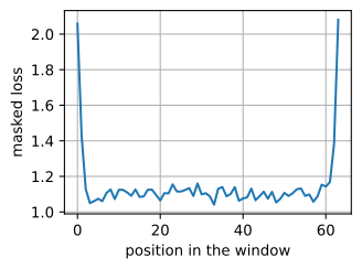
model.eval()

@nnx.jit
def mlm_eval(model, Xm, X):
    logits = model.token_emb.attend(model(Xm))
    losses = optax.softmax_cross_entropy_with_integer_labels(logits, X)
    return losses, logits.argmax(-1)

pos_loss, pos_cnt = jnp.zeros(64), jnp.zeros(64)
correct = total = 0
key = jax.random.key(1)
for rep in range(5):
    for X, _ in data.val_dataloader():
        X = jnp.asarray(X)
        key, sub = jax.random.split(key)
        Xm, mask = mask_tokens(X, sub)
        loss, pred = mlm_eval(model, Xm, X)
        pos_loss += (loss * mask).sum(0)
        pos_cnt += mask.sum(0)
        correct += int(((pred == X) & mask).sum())
        total += int(mask.sum())
pos_loss = pos_loss / pos_cnt
print(f'masked accuracy {correct / total:.2f}')
print(f'loss at position 0: {pos_loss[0]:.2f}, at position 63: '
      f'{pos_loss[63]:.2f}, interior mean: {pos_loss[16:48].mean():.2f}')
d2l.plot(jnp.arange(64), pos_loss, 'position in the window',
         'masked loss')
masked accuracy 0.61
loss at position 0: 2.11, at position 63: 2.20, interior mean: 1.20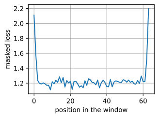
The profile is flat across the interior at about \(1.1\) nats and roughly doubles at the two one-sided edges. That gap is the second side’s value, measured: conditioning on both sides of a character cuts its loss by about half relative to one side, because for text, what follows a gap narrows it down about as sharply as what precedes it. The predictions are readable too — mask a character and the model fills it from its surroundings:
snippet = 'the time traveller for so it will be convenient to speak of him '
ids = torch.tensor(data.vocab[list(snippet)], device=device)[None]
for pos in (9, 14, 30):
    Xm = ids.clone()
    Xm[0, pos] = MASK
    with torch.no_grad():
        logits = F.linear(model(Xm), model.token_emb.weight)
    probs = F.softmax(logits[0, pos], -1)
    top = probs.topk(3)
    shown = snippet[:pos] + '_' + snippet[pos + 1:]
    print(f'{shown[:40]!r}... -> '
          + ', '.join(f'{data.vocab.to_tokens(int(i))!r} {p:.2f}'
                      for p, i in zip(top.values, top.indices)))
'the time _raveller for so it will be con'... -> 't' 0.94, 'g' 0.02, 'f' 0.01
'the time trave_ler for so it will be con'... -> 'l' 0.99, ' ' 0.01, 'r' 0.00
'the time traveller for so it w_ll be con'... -> 'i' 0.63, 'e' 0.29, 'a' 0.06snippet = 'the time traveller for so it will be convenient to speak of him '
ids = jnp.asarray(data.vocab[list(snippet)])[None]
for pos in (9, 14, 30):
Xm = ids.at[0, pos].set(MASK)
probs = jax.nn.softmax(model.token_emb.attend(model(Xm))[0, pos])
top = jnp.argsort(probs)[::-1][:3]
shown = snippet[:pos] + '_' + snippet[pos + 1:]
print(f'{shown[:40]!r}... -> '
+ ', '.join(f'{data.vocab.to_tokens(int(i))!r} {probs[i]:.2f}'
for i in top))'the time _raveller for so it will be con'... -> 't' 0.72, 'g' 0.05, 'f' 0.05
'the time trave_ler for so it will be con'... -> 'l' 0.96, ' ' 0.02, 'r' 0.01
'the time traveller for so it w_ll be con'... -> 'e' 0.46, 'i' 0.40, 'o' 0.09The doubled consonant in “trave_ler” comes back with high confidence: only the right-hand context (“ler”) pins it down, and a left-to-right model would never see it. Scaled up to subword tokens, sentence pairs, gigabytes of text, and a fine-tuning recipe per downstream task, this experiment is BERT (Devlin et al. 2018), whose pretraining and fine-tuning the Language Models part covers in full (Chapter 18). Nor did the wiring stop evolving in 2019: ModernBERT rebuilds the same encoder-only architecture with the modern block internals of this chapter (RoPE, gated FFN, alternating local–global attention, and an 8k context), and it remains the backbone of choice for retrieval and classification at small model sizes (Warner et al. 2024).
11.4.3 An Encoder–Decoder: Cross-Attention at Work
11.4.3.1 A Task Whose Alignment We Know
An encoder–decoder is useful when the input and output are different sequences. Its signature component, cross-attention, is usually illustrated on machine translation, but a trained translation model gives us no ground truth to check its attention against. So we choose a task whose correct alignment is known by construction: reverse a random string. Target position \(t\) must copy source position \(n-1-t\), the letters are drawn independently at random, and the only path from source content to the decoder runs through cross-attention. If the mechanism works and the model solves the task directly, its attention map should be the anti-diagonal — a prediction we can check. Random strings also mean unlimited fresh data: unlike the memorizing GPT of Section 11.2, this model never sees the same example twice.
V, T = 16, 12   # 16 letters, strings of length 12
BOS = V         # decoder start token

def sample_batch(batch_size):
    src = torch.randint(0, V, (batch_size, T), device=device)
    tgt = src.flip(1)
    dec_in = torch.cat([torch.full((batch_size, 1), BOS, device=device),
                        tgt[:, :-1]], 1)
    return src, dec_in, tgt

def to_str(ids):
    return ''.join(chr(97 + int(i)) for i in ids)

src, dec_in, tgt = sample_batch(1)
print(f'source {to_str(src[0])!r} -> target {to_str(tgt[0])!r}')
source 'ioaofaoebgaj' -> target 'jagbeoafoaoi'V, T = 16, 12 # 16 letters, strings of length 12
BOS = V # decoder start token
def sample_batch(batch_size, key):
src = jax.random.randint(key, (batch_size, T), 0, V)
tgt = src[:, ::-1]
dec_in = jnp.concatenate(
[jnp.full((batch_size, 1), BOS), tgt[:, :-1]], 1)
return src, dec_in, tgt
def to_str(ids):
return ''.join(chr(97 + int(i)) for i in ids)
src, dec_in, tgt = sample_batch(1, jax.random.key(0))
print(f'source {to_str(src[0])!r} -> target {to_str(tgt[0])!r}')source 'fainddapflek' -> target 'kelfpaddniaf'As in Section 11.2, training uses teacher forcing: the decoder input is the target shifted right behind a <bos> token, so every position learns to predict its successor in parallel.
11.4.3.2 The Decoder Block: One More Sublayer
A decoder block is the transformer block plus one sublayer. Between the causal self-attention and the FFN sits cross-attention: queries from the target’s residual stream, keys and values from the encoder output. It follows the same pre-norm discipline as everything in this chapter — each sublayer reads the stream through a normalization and adds its result back. Note the masking asymmetry: self-attention stays causal (the target is being generated), while cross-attention is unmasked (the source is fully known before generation starts).
class DecoderBlock(nn.Module):
    """Pre-norm decoder block: causal self-attention, cross-attention,
    FFN."""
    def __init__(self, num_hiddens, num_heads):
        super().__init__()
        self.norm1 = nn.RMSNorm(num_hiddens)
        self.norm2 = nn.RMSNorm(num_hiddens)
        self.norm3 = nn.RMSNorm(num_hiddens)
        self.self_attention = d2l.MultiHeadAttention(num_hiddens, num_heads,
                                                     dropout=0)
        self.cross_attention = d2l.MultiHeadAttention(num_hiddens,
                                                      num_heads, dropout=0)
        self.ffn = d2l.FeedForward(num_hiddens)

    def forward(self, X, enc):
        B, T = X.shape[:2]
        causal = torch.arange(1, T + 1, device=X.device).repeat(B, 1)
        Y = self.norm1(X)
        X = X + self.self_attention(Y, Y, Y, causal)
        X = X + self.cross_attention(self.norm2(X), enc, enc, None)
        return X + self.ffn(self.norm3(X))
class DecoderBlock(nnx.Module):
"""Pre-norm decoder block: causal self-attention, cross-attention,
FFN."""
def __init__(self, num_hiddens, num_heads, rngs=None):
rngs = nnx.Rngs(0) if rngs is None else rngs
self.norm1 = nnx.RMSNorm(num_hiddens, rngs=rngs)
self.norm2 = nnx.RMSNorm(num_hiddens, rngs=rngs)
self.norm3 = nnx.RMSNorm(num_hiddens, rngs=rngs)
self.self_attention = d2l.MultiHeadAttention(num_hiddens, num_heads,
dropout=0, rngs=rngs)
self.cross_attention = d2l.MultiHeadAttention(
num_hiddens, num_heads, dropout=0, rngs=rngs)
self.ffn = d2l.FeedForward(num_hiddens, rngs=rngs)
def __call__(self, X, enc):
B, T = X.shape[:2]
causal = jnp.tile(jnp.arange(1, T + 1), (B, 1))
Y = self.norm1(X)
X = X + self.self_attention(Y, Y, Y, causal)[0]
Y2, cross_weights = self.cross_attention(self.norm2(X), enc, enc,
None)
X = X + Y2
return X + self.ffn(self.norm3(X)), cross_weightsThe full model wires a TransformerEncoder (the class from the previous section, reused unchanged) to a stack of decoder blocks with its own embeddings and output head. Following the framework conventions of Section 10.3, the JAX model returns the cross-attention weights alongside the logits, while the PyTorch model stores them on the attention module.
class EncoderDecoder(nn.Module):
    """A causal decoder cross-attending into a bidirectional encoder."""
    def __init__(self, vocab_size, num_hiddens=128, num_heads=4,
                 num_blks=1, max_len=64):
        super().__init__()
        self.encoder = TransformerEncoder(vocab_size, num_hiddens,
                                          num_heads, num_blks, max_len)
        self.tgt_emb = nn.Embedding(vocab_size, num_hiddens)
        self.pos_emb = nn.Embedding(max_len, num_hiddens)
        for emb in (self.tgt_emb, self.pos_emb):
            nn.init.normal_(emb.weight, std=0.02)
        self.blks = nn.ModuleList([DecoderBlock(num_hiddens, num_heads)
                                   for _ in range(num_blks)])
        self.norm = nn.RMSNorm(num_hiddens)
        self.head = nn.Linear(num_hiddens, vocab_size, bias=False)

    def forward(self, src, dec_in):
        enc = self.encoder(src)
        H = self.tgt_emb(dec_in) + self.pos_emb(
            torch.arange(dec_in.shape[1], device=dec_in.device))
        for blk in self.blks:
            H = blk(H, enc)
        return self.head(self.norm(H))
class EncoderDecoder(nnx.Module):
"""A causal decoder cross-attending into a bidirectional encoder."""
def __init__(self, vocab_size, num_hiddens=128, num_heads=4,
num_blks=1, max_len=64, rngs=None):
rngs = nnx.Rngs(0) if rngs is None else rngs
init = nnx.initializers.normal(0.02)
self.encoder = TransformerEncoder(vocab_size, num_hiddens,
num_heads, num_blks, max_len,
rngs=rngs)
self.tgt_emb = nnx.Embed(vocab_size, num_hiddens,
embedding_init=init, rngs=rngs)
self.pos_emb = nnx.Embed(max_len, num_hiddens, embedding_init=init,
rngs=rngs)
self.blks = nnx.List([DecoderBlock(num_hiddens, num_heads,
rngs=rngs)
for _ in range(num_blks)])
self.norm = nnx.RMSNorm(num_hiddens, rngs=rngs)
self.head = nnx.Linear(num_hiddens, vocab_size, use_bias=False,
rngs=rngs)
def __call__(self, src, dec_in):
enc = self.encoder(src)
H = self.tgt_emb(dec_in) + self.pos_emb(jnp.arange(dec_in.shape[1]))
weights = []
for blk in self.blks:
H, w = blk(H, enc)
weights.append(w)
return self.head(self.norm(H)), weights11.4.3.3 Assembling the Masks
Our reversal task ducks one bookkeeping question by construction: every string has the same length, so nothing is padding, and the only mask in sight is the decoder’s causal one. A real batch needs three masks, one per attention site, because its sequences have different lengths and are padded to a rectangle; each mask is composed from the two primitives of Section 10.2: a padding mask built from valid lengths, and the causal triangle, combined by logical AND under broadcasting. Encoder self-attention masks source padding. Decoder self-attention during teacher-forced training needs the causal triangle and target padding on the key side (padded query rows compute outputs the loss ignores). Cross-attention masks source padding again, since the target may be mid-generation but the source it reads is fully known. The cell below assembles all three for a toy ragged batch, as boolean arrays of shape (batch, queries, keys) — the form the fused kernels of Section 10.5 accept; d2l.MultiHeadAttention’s valid_lens argument carries the same information in compressed form.
src_len, tgt_len = torch.tensor([3, 5]), torch.tensor([3, 4])
S, T_dec = int(src_len.max()), int(tgt_len.max())
src_valid = (torch.arange(S)[None, :] < src_len[:, None])[:, None, :]
tgt_valid = (torch.arange(T_dec)[None, :] < tgt_len[:, None])[:, None, :]
causal = (torch.arange(T_dec)[None, :]
          <= torch.arange(T_dec)[:, None])[None]        # (1, T, T)
enc_self = src_valid.expand(-1, S, -1)     # (B, S, S): source padding
dec_self = causal & tgt_valid              # (B, T, T): causal AND padding
cross = src_valid.expand(-1, T_dec, -1)    # (B, T, S): source padding
for name, m in (('encoder self', enc_self), ('decoder self', dec_self),
                ('cross', cross)):
    print(f'{name}-attention mask, sequence 0 (1 = may attend):')
    print(m[0].int().numpy())
encoder self-attention mask, sequence 0 (1 = may attend):
[[1 1 1 0 0]
[1 1 1 0 0]
[1 1 1 0 0]
[1 1 1 0 0]
[1 1 1 0 0]]
decoder self-attention mask, sequence 0 (1 = may attend):
[[1 0 0 0]
[1 1 0 0]
[1 1 1 0]
[1 1 1 0]]
cross-attention mask, sequence 0 (1 = may attend):
[[1 1 1 0 0]
[1 1 1 0 0]
[1 1 1 0 0]
[1 1 1 0 0]]src_len, tgt_len = jnp.array([3, 5]), jnp.array([3, 4])
S, T_dec = int(src_len.max()), int(tgt_len.max())
src_valid = (jnp.arange(S)[None, :] < src_len[:, None])[:, None, :]
tgt_valid = (jnp.arange(T_dec)[None, :] < tgt_len[:, None])[:, None, :]
causal = (jnp.arange(T_dec)[None, :]
<= jnp.arange(T_dec)[:, None])[None] # (1, T, T)
B = len(src_len)
enc_self = jnp.broadcast_to(src_valid, (B, S, S)) # source padding
dec_self = causal & tgt_valid # (B, T, T): causal AND padding
cross = jnp.broadcast_to(src_valid, (B, T_dec, S)) # source padding
for name, m in (('encoder self', enc_self), ('decoder self', dec_self),
('cross', cross)):
print(f'{name}-attention mask, sequence 0 (1 = may attend):')
print(m[0].astype(int))encoder self-attention mask, sequence 0 (1 = may attend):
[[1 1 1 0 0]
[1 1 1 0 0]
[1 1 1 0 0]
[1 1 1 0 0]
[1 1 1 0 0]]
decoder self-attention mask, sequence 0 (1 = may attend):
[[1 0 0 0]
[1 1 0 0]
[1 1 1 0]
[1 1 1 0]]
cross-attention mask, sequence 0 (1 = may attend):
[[1 1 1 0 0]
[1 1 1 0 0]
[1 1 1 0 0]
[1 1 1 0 0]]Read sequence 0’s three grids (source length 3 of 5, target length 3 of 4): the encoder square and the cross rectangle both blank the same two padded source columns, and the decoder triangle loses its last column to target padding. In this section’s model the composition never surfaces — sample_batch produces no padding, and the cross-attention call passes valid_lens=None — but these three grids are what a production encoder–decoder assembles for every batch it trains on.
11.4.3.4 Training and Decoding
One encoder block, one decoder block, and a few hundred steps of on-line batches suffice — the model sees on the order of a million characters, none twice.
torch.manual_seed(0)
seq2seq = EncoderDecoder(V + 1).to(device)
optimizer = torch.optim.AdamW(seq2seq.parameters(), lr=1e-3,
                              weight_decay=0.0)
losses = []
for step in range(600):
    src, dec_in, tgt = sample_batch(128)
    logits = seq2seq(src, dec_in)
    loss = F.cross_entropy(logits.reshape(-1, V + 1), tgt.reshape(-1))
    optimizer.zero_grad()
    loss.backward()
    optimizer.step()
    losses.append(loss.item())
print('loss at step 100/200/400/600: ' + '/'.join(
    f'{sum(losses[k-20:k]) / 20:.3f}' for k in (100, 200, 400, 600)))
loss at step 100/200/400/600: 0.005/0.001/0.001/0.000seq2seq = EncoderDecoder(V + 1, rngs=nnx.Rngs(0))
optimizer = nnx.Optimizer(seq2seq, optax.adamw(1e-3, weight_decay=0.0),
wrt=nnx.Param)
@nnx.jit
def s2s_step(model, optimizer, src, dec_in, tgt):
def loss_fn(model):
logits, _ = model(src, dec_in)
return optax.softmax_cross_entropy_with_integer_labels(
logits.reshape(-1, logits.shape[-1]), tgt.reshape(-1)).mean()
loss, grads = nnx.value_and_grad(loss_fn)(model)
optimizer.update(model, grads)
return loss
key, losses = jax.random.key(0), []
for step in range(600):
key, sub = jax.random.split(key)
src, dec_in, tgt = sample_batch(128, sub)
losses.append(float(s2s_step(seq2seq, optimizer, src, dec_in, tgt)))
print('loss at step 100/200/400/600: ' + '/'.join(
f'{sum(losses[k-20:k]) / 20:.3f}' for k in (100, 200, 400, 600)))loss at step 100/200/400/600: 0.002/0.001/0.000/0.000Decoding runs the encoder once and the decoder autoregressively: feed <bos>, take the argmax, append, repeat. On a thousand fresh strings the model reverses essentially every one exactly.
seq2seq.eval()
torch.manual_seed(1)
with torch.no_grad():
    src, _, tgt = sample_batch(1000)
    enc = seq2seq.encoder(src)
    out = torch.full((1000, T + 1), BOS, device=device)
    for t in range(T):
        H = seq2seq.tgt_emb(out[:, :t + 1]) + seq2seq.pos_emb(
            torch.arange(t + 1, device=device))
        for blk in seq2seq.blks:
            H = blk(H, enc)
        out[:, t + 1] = seq2seq.head(seq2seq.norm(H))[:, -1].argmax(-1)
pred = out[:, 1:]
print(f'exact match on 1000 fresh strings: '
      f'{(pred == tgt).all(-1).float().mean():.3f}')
print(f'source {to_str(src[0])!r} -> predicted {to_str(pred[0])!r}')
exact match on 1000 fresh strings: 1.000
source 'acppaolbfbak' -> predicted 'kabfbloappca'seq2seq.eval()
@nnx.jit
def next_token(model, enc, buf, t):
H = model.tgt_emb(buf) + model.pos_emb(jnp.arange(buf.shape[1]))
for blk in model.blks:
H, _ = blk(H, enc)
return model.head(model.norm(H))[:, t].argmax(-1)
src, _, tgt = sample_batch(1000, jax.random.key(1))
enc = seq2seq.encoder(src)
buf = jnp.full((1000, T + 1), BOS)
for t in range(T):
buf = buf.at[:, t + 1].set(next_token(seq2seq, enc, buf, t))
pred = buf[:, 1:]
print(f'exact match on 1000 fresh strings: '
f'{(pred == tgt).all(-1).mean():.3f}')
print(f'source {to_str(src[0])!r} -> predicted {to_str(pred[0])!r}')exact match on 1000 fresh strings: 1.000
source 'mpajamgfccab' -> predicted 'baccfgmajapm'The decode loop reuses the fixed-buffer idiom from Section 11.2’s generate: a buffer of the final size, overwritten left to right, keeps every shape static so the jitted step compiles exactly once. The causal mask makes the not-yet-written positions invisible to every query at or before \(t\).
11.4.3.5 Reading the Alignment
We run a batch through the model, extract the cross-attention weights from the decoder block, and compare each target position’s attention against the alignment the task dictates.
with torch.no_grad():
    src, dec_in, tgt = sample_batch(64)
    seq2seq(src, dec_in)
w = seq2seq.blks[0].cross_attention.attention.attention_weights
w = w.reshape(64, 4, T, T)
want = torch.arange(T - 1, -1, -1, device=device)  # row t -> column T-1-t
hit = (w.mean(1).argmax(-1) == want).float().mean()
mass = w.mean(1).gather(-1, want.expand(64, T)[..., None]).mean()
print(f'head-averaged argmax hits the true source position on '
      f'{100 * hit:.0f}% of rows; mean weight there {mass:.2f}')
d2l.show_heatmaps(w[0].cpu()[None], xlabel='source position',
                  ylabel='target position',
                  titles=[f'Head {i}' for i in range(1, 5)],
                  figsize=(9, 2.5), cmap='Blues')
head-averaged argmax hits the true source position on 100% of rows; mean weight there 0.88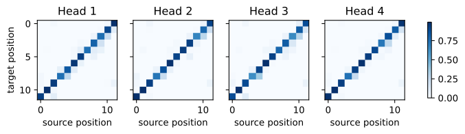
src, dec_in, tgt = sample_batch(64, jax.random.key(2))
_, cross_weights = seq2seq(src, dec_in)
w = cross_weights[0].reshape(64, 4, T, T)
want = jnp.arange(T - 1, -1, -1)                   # row t -> column T-1-t
hit = (w.mean(1).argmax(-1) == want).mean()
mass = jnp.take_along_axis(w.mean(1),
                           jnp.tile(want, (64, 1))[..., None], -1).mean()
print(f'head-averaged argmax hits the true source position on '
      f'{100 * hit:.0f}% of rows; mean weight there {mass:.2f}')
d2l.show_heatmaps(w[0][None], xlabel='source position',
                  ylabel='target position',
                  titles=[f'Head {i}' for i in range(1, 5)],
                  figsize=(9, 2.5), cmap='Blues')
head-averaged argmax hits the true source position on 92% of rows; mean weight there 0.87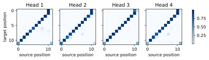
The maps contain the anti-diagonal predicted by the third panel of Figure 11.4.1. Averaged over heads, the argmax lands on the true source position for well over nine rows in ten, with most of the softmax mass concentrated there. The cross-attention therefore represents the alignment built into the task. As Section 10.3 noted, such readable attention patterns are the exception rather than the rule. It is readable here because we made the model small; give the encoder and decoder more depth and heads and the task stays solved while the maps delocalize, as one of the exercises demonstrates.
11.4.4 Cross-Attention as Interface
11.4.4.1 Queries Need Not Come from a Sequence
In the decoder, the cross-attention queries came from the target stream. Nothing in the mechanism requires that source. A set of \(M\) query vectors can instead be learned parameters — a fixed array that exists before any input arrives. Cross-attending it into an input of length \(N\) costs \(O(MN)\); the quadratic term of Section 10.5 never appears, because the \(M\) latents only ever self-attend among themselves at \(O(M^2)\). This is the Perceiver (Jaegle et al. 2021): a fixed-size latent bottleneck that reads arbitrarily long, arbitrarily structured inputs through cross-attention, sketched in Figure 11.4.2.
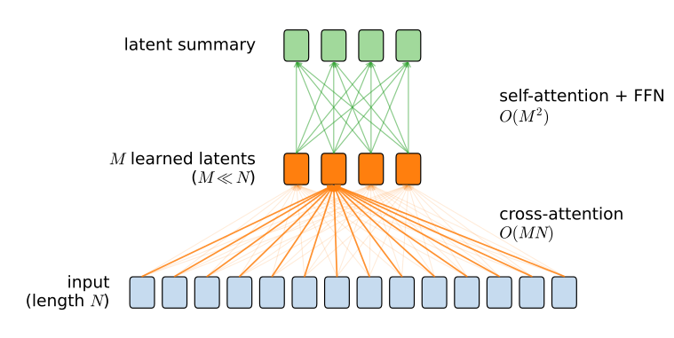
A minimal version needs a parameter array, one cross-attention, and a stack of ordinary transformer blocks over the latents:
class PerceiverEncoder(nn.Module):
    """M learned latents cross-attend into the input, then process among
    themselves."""
    def __init__(self, num_latents, num_hiddens, num_heads=4, num_blks=2):
        super().__init__()
        self.latents = nn.Parameter(
            0.02 * torch.randn(num_latents, num_hiddens))
        self.norm_q = nn.RMSNorm(num_hiddens)
        self.cross_attention = d2l.MultiHeadAttention(num_hiddens,
                                                      num_heads, dropout=0)
        self.blks = nn.ModuleList([
            d2l.TransformerBlock(num_hiddens, num_heads)
            for _ in range(num_blks)])
        self.norm = nn.RMSNorm(num_hiddens)

    def forward(self, X):
        Z = self.latents.expand(X.shape[0], -1, -1)
        Z = Z + self.cross_attention(self.norm_q(Z), X, X, None)  # O(MN)
        for blk in self.blks:
            Z = blk(Z)                                            # O(M^2)
        return self.norm(Z)

perceiver = PerceiverEncoder(num_latents=64, num_hiddens=256).to(device)
X = torch.randn(1, 4096, 256, device=device)
print('input', tuple(X.shape), '-> latent summary',
      tuple(perceiver(X).shape))
input (1, 4096, 256) -> latent summary (1, 64, 256)class PerceiverEncoder(nnx.Module):
"""M learned latents cross-attend into the input, then process among
themselves."""
def __init__(self, num_latents, num_hiddens, num_heads=4, num_blks=2,
rngs=None):
rngs = nnx.Rngs(0) if rngs is None else rngs
self.latents = nnx.Param(
0.02 * jax.random.normal(rngs.params(),
(num_latents, num_hiddens)))
self.norm_q = nnx.RMSNorm(num_hiddens, rngs=rngs)
self.cross_attention = d2l.MultiHeadAttention(
num_hiddens, num_heads, dropout=0, rngs=rngs)
self.blks = nnx.List([
d2l.TransformerBlock(num_hiddens, num_heads, rngs=rngs)
for _ in range(num_blks)])
self.norm = nnx.RMSNorm(num_hiddens, rngs=rngs)
def __call__(self, X):
Z = jnp.broadcast_to(self.latents[...],
(X.shape[0],) + self.latents.shape)
Z = Z + self.cross_attention(self.norm_q(Z), X, X, None)[0] # O(MN)
for blk in self.blks:
Z = blk(Z) # O(M^2)
return self.norm(Z)
perceiver = PerceiverEncoder(num_latents=64, num_hiddens=256)
perceiver.eval()
X = jax.random.normal(jax.random.key(0), (1, 4096, 256))
print('input', X.shape, '-> latent summary', perceiver(X).shape)input (1, 4096, 256) -> latent summary (1, 64, 256)Whatever the input length, the output is \(M = 64\) vectors. The input here is a raw feature sequence rather than token embeddings, because the whole point is indifference to what the input is — text, audio frames, image pixels, or a concatenation of all three.
11.4.4.2 The Cost Curve
The claim to verify is the shape of the cost. We time the Perceiver against the direct alternative (the same two transformer blocks applied to the full input sequence) as \(N\) doubles at fixed \(M = 64\).
class SelfAttentionEncoder(nn.Module):
    """The comparison: the same blocks over the full input sequence."""
    def __init__(self, num_hiddens, num_heads=4, num_blks=2):
        super().__init__()
        self.blks = nn.ModuleList([
            d2l.TransformerBlock(num_hiddens, num_heads)
            for _ in range(num_blks)])

    def forward(self, X):
        for blk in self.blks:
            X = blk(X)                                            # O(N^2)
        return X

full = SelfAttentionEncoder(256).to(device).eval()
perceiver.eval()

def timed(model, X, reps=20):
    with torch.no_grad():
        for _ in range(3):
            model(X)
        if device.type == 'cuda':
            torch.cuda.synchronize()
        t0 = time.time()
        for _ in range(reps):
            model(X)
        if device.type == 'cuda':
            torch.cuda.synchronize()
    return (time.time() - t0) / reps * 1e3

lengths, t_full, t_perc = (1024, 2048, 4096, 8192), [], []
for N in lengths:
    X = torch.randn(1, N, 256, device=device)
    t_full.append(timed(full, X))
    t_perc.append(timed(perceiver, X))
    print(f'N={N:5d}: self-attention {t_full[-1]:6.2f} ms, '
          f'perceiver {t_perc[-1]:5.2f} ms')
d2l.plot(list(lengths), [t_full, t_perc], 'input length N',
         'forward time (ms)', xscale='log', yscale='log',
         legend=['self-attention encoder', 'perceiver encoder'])
N= 1024: self-attention 0.99 ms, perceiver 1.31 ms
N= 2048: self-attention 2.80 ms, perceiver 1.40 ms
N= 4096: self-attention 9.46 ms, perceiver 1.35 ms
N= 8192: self-attention 34.79 ms, perceiver 1.72 ms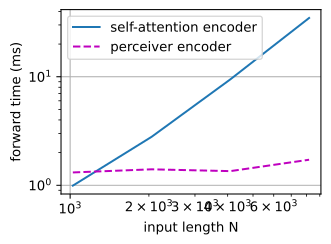
class SelfAttentionEncoder(nnx.Module):
    """The comparison: the same blocks over the full input sequence."""
    def __init__(self, num_hiddens, num_heads=4, num_blks=2, rngs=None):
        rngs = nnx.Rngs(0) if rngs is None else rngs
        self.blks = nnx.List([
            d2l.TransformerBlock(num_hiddens, num_heads, rngs=rngs)
            for _ in range(num_blks)])

    def __call__(self, X):
        for blk in self.blks:
            X = blk(X)                                            # O(N^2)
        return X

full = SelfAttentionEncoder(256)
full.eval()
jit_full, jit_perc = nnx.jit(full), nnx.jit(perceiver)

def timed(f, X, reps=20):
    f(X).block_until_ready()  # warmup + compile
    t0 = time.time()
    for _ in range(reps):
        Y = f(X)
    Y.block_until_ready()
    return (time.time() - t0) / reps * 1e3

lengths, t_full, t_perc = (1024, 2048, 4096, 8192), [], []
for N in lengths:
    X = jax.random.normal(jax.random.key(0), (1, N, 256))
    t_full.append(timed(jit_full, X))
    t_perc.append(timed(jit_perc, X))
    print(f'N={N:5d}: self-attention {t_full[-1]:6.2f} ms, '
          f'perceiver {t_perc[-1]:5.2f} ms')
d2l.plot(list(lengths), [t_full, t_perc], 'input length N',
         'forward time (ms)', xscale='log', yscale='log',
         legend=['self-attention encoder', 'perceiver encoder'])
N= 1024: self-attention 0.33 ms, perceiver 0.23 ms
N= 2048: self-attention 0.62 ms, perceiver 0.34 ms
N= 4096: self-attention 2.69 ms, perceiver 0.16 ms
N= 8192: self-attention 10.00 ms, perceiver 0.27 ms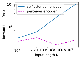
Each doubling of \(N\) eventually multiplies the self-attention encoder’s time by about four, the signature of an \(N^2\) term taking over. The Perceiver’s time grows more slowly over this range (its \(O(MN)\) cross-attention grows linearly but remains dominated by the fixed \(O(M^2)\) latent processing), and by \(N = 8192\) the gap exceeds an order of magnitude. At the left end of the plot, the Perceiver’s fixed \(O(M^2)\) latent cost is a large fraction of the total, so its margin is slim — and with PyTorch’s kernels full self-attention is actually faster at \(N = 1024\). A latent bottleneck is advantageous when the input is long and a fixed-size summary suffices.
11.4.4.3 Perceiver IO and the Idea’s Descendants
Learned queries can also determine the output structure. Perceiver IO (Jaegle et al. 2022) adds an output query array that cross-attends out of the latent summary, so the output size and shape are set by the queries rather than by the input — one query for a classification label, one per pixel for optical flow, one per audio sample for a waveform. Input length, latent width, and output shape become three independent choices, while the latent transformer retains a fixed cost.
The pattern’s descendants run through today’s multimodal systems. Flamingo’s Perceiver resampler compresses a variable number of image and video features into a fixed handful of visual tokens before a frozen language model ever sees them (Alayrac et al. 2022); BLIP-2’s Q-Former is a small stack of learned query tokens that bridges a frozen vision encoder and a frozen LLM (Li et al. 2023); learned query tokens remain one of the two standard interfaces in current vision–language models — the other is a plain learned projection applied patch by patch. DETR had already used the query-token device for detection — a hundred learned object queries cross-attend into image features, each producing one detection (Carion et al. 2020). The Image Models part (Chapter 20) takes up DETR and its successors in depth.
11.4.5 Choosing an Architecture
The taxonomy of Figure 11.4.1 describes several widely used model families. The table gives examples rather than an exhaustive ranking.
| Wiring | Exemplars today | Typical use |
|---|---|---|
| encoder-only | BERT descendants, ModernBERT | embeddings, retrieval, classification |
| encoder–decoder | T5 family, Whisper | translation, speech recognition |
| decoder-only | GPT-style models | generation, chat, in-context learning |
Encoder-only models remain useful when the output is a representation. An embedding model processes each document once and can use bidirectional context, so retrieval and reranking systems still train BERT-shaped models (Warner et al. 2024). The encoder–decoder survives where the input is fully known before generation starts and deserves its own tower: T5-style text-to-text (Raffel et al. 2020), and Whisper, whose encoder reads an entire audio clip bidirectionally while a text decoder cross-attends into it (Radford et al. 2023).
Decoder-only models cover many generative applications. A single stack supports a single pretraining objective: next-token prediction on raw text, with no masking or span-corruption objective. The same stack supplies the states used for next-token generation, and sufficiently large decoder-only models can perform tasks specified in the prompt (Brown et al. 2020). This shared training and serving interface is operationally convenient, but it does not make decoder-only models preferable for every representation or conditional generation task.
11.4.6 Summary
A transformer block supports encoder-only, decoder-only, and encoder–decoder architectures. Removing the causal mask produces an encoder that represents each token using context from both directions. In our character-level experiment, positions with context on both sides have roughly half the loss of positions with only left context. An encoder–decoder connects an unmasked encoder to a causal decoder through cross-attention; on a reversal task, the learned attention map recovers the known anti-diagonal alignment. Cross-attention can also use a learned latent array as its queries. Reading a length-\(N\) input into \(M\) latents costs \(O(MN)\) rather than \(O(N^2)\), and its measured runtime remains nearly constant as \(N\) grows for fixed \(M\). Encoder-only models are common for retrieval and classification, encoder–decoders for translation and speech, and decoder-only models for general autoregressive generation.
11.4.7 Exercises
- Prefix language model. A prefix language model wires a single stack in a fourth way. The first \(m\) positions, which hold the source, attend to one another bidirectionally, and each of the \(n\) target positions that follow attends to the whole source and causally to the target positions up to itself. Raffel et al. (2020) compare this wiring with the encoder–decoder.
- Draw its attention pattern for \(m = 3\) and \(n = 3\) in the convention of Figure 11.4.1. Give the
valid_lensof shape (batch size, number of queries) that makesd2l.MultiHeadAttentionapply this pattern, as a formula in the query position \(t\) and \(m\). - In the encoder–decoder, the cross-attention of every decoder block reads the output of the last encoder block. Which representations of the source does a target token read in block \(l\) of a prefix language model? On which tokens can a source token’s representation depend in each design?
- Let every block have \(c\) parameters, each applied once to every token that the block processes, and ignore the cross-attention sublayer and the attention scores. Compare the parameter count and the training FLOPs per example of an encoder–decoder with \(L\) encoder blocks and \(L\) decoder blocks against prefix language models with \(L\) blocks and with \(2L\) blocks. Which prefix model matches the encoder–decoder in parameters, and which in compute?
- Draw its attention pattern for \(m = 3\) and \(n = 3\) in the convention of Figure 11.4.1. Give the
- [code] A leaky objective. Without a mask, next-token prediction is a copying exercise for an encoder, because position \(t\) can read token \(t + 1\) directly. Train
TransformerEncoderon next-token prediction anyway: feed it the unmodified windowsX, score its predictions at every position against the shifted targetsYthat the data loader returns, and train for 2000 steps with the optimizer settings used formodel.- Predict the validation loss at each position before training. Then plot the measured loss by position as in Section 11.4.2.3.
- Compare the loss at position 63 with the loss of
modelat the same position. For each of the two models, count the training targets per window that cannot be read off the input, at position 63 and in total, and explain the difference.
- Time’s arrow. ● The masked loss of Section 11.4.2.3 takes nearly equal values at the two edges of the window, although position 0 sees only what follows it and position 63 only what precedes it. The conditional entropy \(H(A \mid B) = -\mathbb{E}\left[\log p(A \mid B)\right]\) is the expected loss, in nats, of the best predictor of \(A\) from \(B\).
- Let \(X_1, X_2, \ldots\) be a stationary process, so that the joint distribution of any \(k\) consecutive variables does not depend on where the block starts. Show that \[H(X_1 \mid X_2, \ldots, X_{k+1}) = H(X_{k+1} \mid X_1, \ldots, X_k).\]
- A stationary Markov chain on the states \(\{0, 1, 2\}\) moves from state \(i\) to state \(i + 1 \bmod 3\) with probability \(0.9\) and stays with probability \(0.1\). Compute both sides of the identity for \(k = 1\) in nats. Find the transition matrix of the time-reversed chain, and decide whether a long sample path reveals the direction of time.
- State what the identity predicts for the two edge losses of a model whose masked-token predictions equal the true conditional distributions. Which differences between the experiment and the assumptions of the identity allow the two measured edge losses to differ?
- [code] The masking recipe.
mask_tokensmasks 15% of the characters and writes<mask>at every masked position. Evaluate every variant below with the evaluation of Section 11.4.2.3, so that only the training recipe changes.- BERT replaces a chosen token with
<mask>80% of the time, with a random token 10% of the time, and leaves it unchanged 10% of the time (Devlin et al. 2018), in part because<mask>never appears when the pretrained encoder reads real text. Implement this rule, retrain, and compare the masked accuracy with that of the original recipe. Then feed both encoders unmodified validation windows and measure the loss of predicting each input character at its own position. Explain what each of the two 10% cases teaches the model. - Wettig et al. (2023) find that masking rates well above 15% can work better for large models. Retrain with the rates \(p \in \{0.05, 0.15, 0.4\}\) for the same number of steps and compare the masked loss at evaluation. Explain the result by what a higher rate adds to each training window and what it removes.
- BERT replaces a chosen token with
- [code] Several masks at once. ● The objective Equation 11.4.1 scores each masked position separately, so the encoder returns one distribution per masked position, conditioned only on the characters that remain visible. Filling all masked positions from one forward pass therefore chooses each character independently of the others. Iterative schemes such as Mask-Predict (Ghazvininejad et al. 2019) keep only their most confident predictions and predict the remaining positions again.
- Construct a distribution over the two-character fills of a gap for which the pair of per-position argmaxes has probability zero. Show that filling the more confident position first and then filling the other from its exact conditional distribution always yields a pair of positive probability.
- In each validation window, mask one run of \(k\) adjacent characters, placed at random with at least 8 unmasked characters on either side, and nothing else. For \(k \in \{1, 2, 4, 8\}\), measure the character accuracy of the parallel fill and of an iterative fill that commits one character per forward pass, always at the masked position whose top probability is largest.
- Plot the accuracy of both fills against the offset within the run. Explain the shape of the curves by the context that each masked character has lost, and explain where the two fills differ.
- Padding masks of a ragged batch. The cell of Section 11.4.3.3 builds the three masks for a toy batch with source lengths \((3, 5)\) and target lengths \((3, 4)\), padded on the right.
- Compare
dec_selfwith the causal triangle alone and name the rows that differ. Would replacingdec_selfby the causal triangle change the training loss of a decoder with any number of blocks? Explain. Then decide whether the encoder output at a padded source position can reach the loss. - Now pad the batch on the left, so that every sequence ends at the last position. Which of the three masks change, and does the causal triangle still suffice for decoder self-attention? Which of the three masks can the
valid_lensargument ofd2l.MultiHeadAttentionstill express? - What goes wrong with the learned position tables of
EncoderDecoderunder left padding unless the position indices change as well?
- Compare
- [code] Where position enters. ● Cross-attention without a mask is invariant to a joint permutation of its keys and values, so the reversal task of Section 11.4.3.1 is solvable only because the source representations carry position.
EncoderDecodersupplies position to both streams through learned tables.- Remove the position embedding from the encoder, retrain on reversal, and measure the accuracy of the teacher-forced predictions
seq2seq(src, dec_in)at each target position on fresh strings. - Without position, the encoder output determines at most the multiset of source letters. For 16 letters and strings of length 12, compute the best accuracy at each target position that a predictor can reach when it knows this multiset and the correct target prefix. Compare it with your measurement.
- Restore the encoder’s position table and remove the decoder’s instead. Measure the exact match after greedy decoding, and explain from which part of the decoder its position information can come.
- Remove the position embedding from the encoder, retrain on reversal, and measure the accuracy of the teacher-forced predictions
- [code] Depth, heads, and readable maps. The alignment check of Section 11.4.3.5 reads one decoder block with four heads.
- Retrain
EncoderDecoderonce withnum_blks=2and once withnum_heads=8, in each case until the exact match on 1000 fresh strings exceeds 0.99. Rerun the alignment check for every decoder block, and plot the map of every head. - Give
EncoderDecoderseparate depths for its encoder and its decoder. Repeat the check with two encoder blocks and one decoder block, and with one encoder block and two decoder blocks. Compare the maps of both models with those of the one-block model. - Explain how a model can solve reversal while its cross-attention puts little weight on source position \(n - 1 - t\). Reconcile your findings with the cautions about reading attention maps in Section 10.3.
- Retrain
- [code] Content-addressed alignment. ● In reversal, target position \(t\) copies the same source position for every string. Change the line of
sample_batchthat builds the target so that the target is the source sorted in increasing order.- For one string with a repeated letter, list the source positions that each target position may copy. Redefine the hit rate of Section 11.4.3.5 so that every correct choice counts.
- Train
EncoderDecoderon sorting with one block and with two blocks, for as many steps as the exact match on fresh strings requires or until it stops improving. Report the exact match and your hit rate. - Plot the maps for two strings. Describe what the decoder’s query at step \(t\) must encode for sorting, compared with reversal, and which information the encoder must supply when a letter occurs more than once.
- [code] FLOPs versus time. ● The caption of Figure 11.4.2 counts only the attention mixing, whereas the cost curve of Section 11.4.4.2 times whole forward passes.
- Count the FLOPs of one forward pass of
PerceiverEncoderand ofSelfAttentionEncoderon a batch of one, as functions of \(N\), \(M\), \(d\), and the number of blocks \(L\), with one multiply–add counted as two FLOPs as in Equation 10.3.3. Include the query, key, value, and output projections and the SwiGLU FFN ofd2l.FeedForward. Evaluate both counts for \(d = 256\), \(L = 2\), and \(M = 64\) at the four input lengths of the cost curve. Which term dominates the Perceiver’s count? - Compare the ratio of the two counts at each \(N\) with the ratio of your measured times. Where do the two ratios disagree most, and which part of the running time does a count of arithmetic leave out?
- Repeat the timing for \(M \in \{16, 64, 256\}\) at the input lengths \(N \in \{128, 256, \ldots, 8192\}\). How does the input length at which the Perceiver becomes the faster model move with \(M\), and does your count explain the movement?
- Perceiver IO (Jaegle et al. 2022) adds \(K\) learned output queries that cross-attend into the \(M\) latents. Add their cost to your count. For one output per input element, \(K = N\), as in optical flow, state how the total grows with \(N\) and compare it with the count of
SelfAttentionEncoder.
- Count the FLOPs of one forward pass of
- [extended] A Perceiver for reversal. ● Perceiver IO produces its outputs through learned output queries rather than an autoregressive decoder. Solve the reversal task of Section 11.4.3.1 in this way, with
num_hiddens=128throughout.- Embed the source with learned letter and position tables and read it with
PerceiverEncoderinto \(M\) latents. Let 12 learned output queries, one per target position, cross-attend into the latent summary, and add each result to its query. Applyd2l.FeedForwardwith a second residual connection, and map the result linearly onto the 16 letters. Train all outputs in parallel with the cross-entropy loss on fresh batches fromsample_batch, with no decoder input. - Train with \(M \in \{1, 2, 4, 12\}\) for a fixed number of steps and report the exact match on 1000 fresh strings. Find the smallest \(M\) that solves the task. For a smaller \(M\), decide whether the latents’ read of the source or the output queries’ read of the latents limits the model.
- Plot the latents’ cross-attention over the source and the output queries’ attention over the latents. Describe how the model divides the string among the latents.
- Explain why predicting all target positions independently given the latents is no restriction for reversal, and name a sequence task for which it would be one.
- Embed the source with learned letter and position tables and read it with