rng = np.random.default_rng()
n, d, nu = 200, 5, 0.1
w_true = np.array([1.0, -2.0, 1.5, 0.0, 2.0])
X = rng.normal(size=(n, d))
y = np.where(rng.random(n) < 1 / (1 + np.exp(-X @ w_true)), 1.0, -1.0)

def loss(w, X, y, nu):
    return np.logaddexp(0, -y * (X @ w)).mean() + nu / 2 * (w @ w)

def grad_rows(w, X, y, nu):                   # row i: gradient of example i
    s = 1 / (1 + np.exp(y * (X @ w)))         # sigmoid(-y_i x_i^T w)
    return -(y * s)[:, None] * X + nu * w

w_star = np.zeros(d)
for _ in range(4000):                         # full-batch reference optimum
w_star = w_star - 0.5 * grad_rows(w_star, X, y, nu).mean(axis=0)35.2 Curvature Methods: Newton, Quasi-Newton, and Trust Regions
Gradient descent never looks at the curvature of the function it descends. It only suffers from it: the steepest direction caps the step, the flattest direction then crawls, and the number of steps grows with the condition number \(\kappa\), or with \(\sqrt\kappa\) once momentum is added (Section 35.1.3). On the chapter’s running example \(\tfrac12(x_1^2 + 1000\,x_2^2)\) that came to \(6{,}908\) steps, or \(315\) with momentum. Yet anyone can solve this problem by inspection: divide each coordinate of the gradient by its curvature, \(1\) or \(1000\), and a single step lands on the minimum. What does a method gain when it measures the curvature instead of merely surviving it?
Newton’s method, a century and a half older than gradient descent, is the classical answer. It fits a quadratic to the function at the current point and jumps to the minimum of the quadratic. We ask four questions of it. How fast is it? What does a step cost? Where does it go wrong? And how much of it can be recovered from gradients alone, when second derivatives are out of reach? In brief: it is very fast near a minimum, it is far too expensive for a network, it runs to saddle points as readily as to minima, and a good part of it can be rebuilt by comparing successive gradients. The remedy for the saddles is to limit each step to the region where the quadratic has predicted well.
For training networks this section matters less than the previous one, and we should say so. A Hessian is too large to form, and minibatch noise spoils curvature estimates built from differences of gradients. The ideas return in other forms, though: the per-coordinate steps of Adam are a diagonal stand-in for Newton’s matrix (Section 35.5), and the damping that such methods add to a curvature matrix is the shift of a trust region. The result to remember is the quadratic convergence of Newton’s method Equation 35.2.3. The part on quasi-Newton methods can be skipped on a first reading. From Section 35.1 we reuse two things: the Armijo test of the backtracking line search, and the function \(\tfrac12 x^2 + \cos y\), at whose saddle gradient descent stopped.
35.2.1 Newton’s Method
Gradient descent rests on a linear model of \(f\). A linear model has no minimum, which is why the method needs a step size from outside. A quadratic model has a minimum of its own, and with it comes a step that needs no tuning.
35.2.1.1 The Newton Step
Newton’s method lets the curvature choose the step (Section 9.2.3). Model \(f\) near \(\mathbf{x}_k\) by its second-order Taylor expansion in the step \(\mathbf{p}\):
\[ m_k(\mathbf{p}) = f(\mathbf{x}_k) + \mathbf{g}_k^\top \mathbf{p} + \tfrac12\, \mathbf{p}^\top \nabla^2 f(\mathbf{x}_k)\, \mathbf{p}. \tag{35.2.1}\]
If \(\nabla^2 f(\mathbf{x}_k)\) is positive definite, the model is a bowl with a unique minimizer, where \(\nabla m_k = \mathbf{g}_k + \nabla^2 f(\mathbf{x}_k)\,\mathbf{p} = \mathbf{0}\). Solving for \(\mathbf{p}\) and stepping there is Newton’s method:
\[ \mathbf{x}_{k+1} = \mathbf{x}_k - \big(\nabla^2 f(\mathbf{x}_k)\big)^{-1} \nabla f(\mathbf{x}_k). \tag{35.2.2}\]
No step size appears: the curvature has set it. Newton’s direction belongs to the family \(\mathbf{d} = -\mathbf{P}^{-1}\nabla f\) with a positive definite matrix \(\mathbf{P}\), here \(\nabla^2 f\). Every member of the family is a descent direction, since \(\nabla f^\top \mathbf{d} = -\nabla f^\top \mathbf{P}^{-1}\nabla f < 0\). Newton’s direction is the steepest one when lengths are measured in the Hessian’s norm instead of the Euclidean one (exercise 1).
On the quadratic \(\tfrac12\mathbf{x}^\top\mathbf{A}\mathbf{x}\) the model is the function, so one step lands on the minimizer, \(\mathbf{x}_1 = \mathbf{x}_0 - \mathbf{A}^{-1}\mathbf{A}\mathbf{x}_0 = \mathbf{0}\), for every \(\kappa\). The reason goes deeper than the algebra. Newton’s method is affine-invariant: it does not depend on the coordinates. Under a change of coordinates \(\mathbf{x} = \mathbf{T}\mathbf{y}\), Newton’s iterates for \(f(\mathbf{T}\mathbf{y})\) are the images of Newton’s iterates for \(f\). Gradient descent’s iterates, in contrast, change under every \(\mathbf{T}\) that is not orthogonal; a multiple of an orthogonal matrix changes only the effective step (exercise 1). Since a change of coordinates can make any positive definite quadratic round, the condition number cannot matter to Newton. A long valley is, to Newton’s method, a round bowl drawn on stretched paper.
35.2.1.2 Quadratic Convergence
On a function that is not quadratic the model is only an approximation, and one step no longer suffices. What survives is the speed. Near a minimizer Newton’s method converges much faster than geometrically, and the proof is a single use of the fundamental theorem of calculus. We write \(\mathbf{e}_k = \mathbf{x}_k - \mathbf{x}^\star\) for the error.
Proposition (quadratic convergence). Let \(\nabla f(\mathbf{x}^\star) = \mathbf{0}\), and suppose that on a ball around \(\mathbf{x}^\star\) the Hessian satisfies \(\nabla^2 f(\mathbf{x}) \succeq \mu\mathbf{I}\) and \(\|\nabla^2 f(\mathbf{x}) - \nabla^2 f(\mathbf{y})\| \le L_2\|\mathbf{x} - \mathbf{y}\|\). If \(\mathbf{x}_k\) lies in the ball, then
\[ \|\mathbf{e}_{k+1}\| \;\le\; \frac{L_2}{2\mu}\, \|\mathbf{e}_k\|^2. \tag{35.2.3}\]
Proof. Write \(\nabla^2 f_k = \nabla^2 f(\mathbf{x}_k)\). Since \(\nabla f(\mathbf{x}^\star) = \mathbf{0}\), the Newton step gives \(\mathbf{e}_{k+1} = \mathbf{e}_k - (\nabla^2 f_k)^{-1}\mathbf{g}_k = (\nabla^2 f_k)^{-1}\big[\nabla^2 f_k\,\mathbf{e}_k - (\nabla f(\mathbf{x}_k) - \nabla f(\mathbf{x}^\star))\big]\). By the fundamental theorem of calculus along the segment from \(\mathbf{x}^\star\) to \(\mathbf{x}_k\), the gradient difference is \(\int_0^1 \nabla^2 f(\mathbf{x}^\star + t\mathbf{e}_k)\,\mathbf{e}_k\,dt\), so the bracket is \(\int_0^1 \big[\nabla^2 f_k - \nabla^2 f(\mathbf{x}^\star + t\mathbf{e}_k)\big]\mathbf{e}_k\,dt\). The two points differ by \((1 - t)\mathbf{e}_k\), so the bracket has norm at most \(\int_0^1 L_2(1 - t)\|\mathbf{e}_k\|^2\,dt = \tfrac{L_2}{2}\|\mathbf{e}_k\|^2\). Finally \(\|(\nabla^2 f_k)^{-1}\| \le 1/\mu\). \(\blacksquare\)
Multiplying both sides by \(L_2/(2\mu)\) gives \(\tfrac{L_2}{2\mu}\|\mathbf{e}_{k+1}\| \le \big(\tfrac{L_2}{2\mu}\|\mathbf{e}_k\|\big)^2\), so the scaled error squares at every step. If it starts below \(1\), the error shrinks and every later iterate stays in the ball. Once it is below \(0.1\), it goes to \(10^{-2}\), \(10^{-4}\), \(10^{-8}\), so the number of correct digits roughly doubles per step. Compare gradient descent on the running example, which gains one digit in about \(1{,}150\) steps. The speed has a condition attached, and it is in the hypotheses: the bound says nothing until the iterate is already close.
Far from \(\mathbf{x}^\star\) the full step can overshoot, even with a positive definite Hessian. The remedy is damping: step to \(\mathbf{x}_k + \alpha_k\mathbf{p}_k\) along the Newton direction \(\mathbf{p}_k = -(\nabla^2 f(\mathbf{x}_k))^{-1}\mathbf{g}_k\), with \(\alpha_k \le 1\) chosen by backtracking on the Armijo test \(f(\mathbf{x}_k + \alpha\mathbf{p}_k) \le f(\mathbf{x}_k) + c\,\alpha\,\mathbf{g}_k^\top\mathbf{p}_k\), which is Equation 35.1.7 for a general descent direction. Near a minimizer with positive definite Hessian the full step \(\alpha = 1\) passes this test when \(c < \tfrac12\), so damping costs nothing once the fast phase begins.
The test problem for the cells below is \(\ell_2\)-regularized logistic regression on \(n = 200\) random examples in \(d = 5\) dimensions,
\[ f(\mathbf{w}) = \frac1n \sum_{i=1}^n \log\big(1 + \exp(-y_i\,\mathbf{x}_i^\top \mathbf{w})\big) + \frac{\nu}{2}\|\mathbf{w}\|^2, \qquad \nu = 0.1, \]
with labels \(y_i = \pm 1\) drawn from a logistic model (the weight-decay coefficient is \(\nu\) here because \(\lambda\) denotes eigenvalues). The data cell also computes a reference optimum \(\mathbf{w}^\star\) with \(4{,}000\) gradient steps of size \(\eta = 0.5\), which is safe since \(L = \lambda_{\max}(\mathbf{X}^\top\mathbf{X})/(4n) + \nu\) is about \(0.4\) here (exercise 2).
Two predictions can now be tested. On the chapter’s running example \(\mathrm{diag}(1, 1000)\) one Newton step should replace the \(\log 10^6/\log(1001/999) \approx 6{,}908\) steps of gradient descent at its best fixed step (Section 35.1.3). On the logistic loss, which is not a quadratic, the exponent of the gradient norm should roughly double per iteration once the fast phase has begun.
A2 = np.diag([1.0, 1000.0])                   # the running example, kappa = 1000
x = np.array([1.0, 1.0])
x_new = x - np.linalg.solve(A2, A2 @ x)       # one Newton step
rate = (1000 - 1) / (1000 + 1)
print(f'Newton on the quadratic: |x_1| = {np.linalg.norm(x_new):.1e} after one step')
print(f'GD at the optimal step contracts by {rate:.4f}; it needs '
      f'{int(np.ceil(np.log(1e-6) / np.log(rate)))} steps for |x_k| <= 1e-6 |x_0|')
w = np.zeros(d)                               # Newton on the logistic loss
for it in range(6):
    s = 1 / (1 + np.exp(y * (X @ w)))
    g = grad_rows(w, X, y, nu).mean(axis=0)
    hess = (X * (s * (1 - s))[:, None]).T @ X / n + nu * np.eye(d)
    w = w - np.linalg.solve(hess, g)
    print(f'Newton iteration {it + 1}:  |grad| = {np.linalg.norm(g):.1e}')
print(f'max |w - w_star| = {np.abs(w - w_star).max():.1e}')Newton on the quadratic: |x_1| = 0.0e+00 after one step
GD at the optimal step contracts by 0.9980; it needs 6908 steps for |x_k| <= 1e-6 |x_0|
Newton iteration 1: |grad| = 3.5e-01
Newton iteration 2: |grad| = 4.1e-02
Newton iteration 3: |grad| = 1.7e-03
Newton iteration 4: |grad| = 3.0e-06
Newton iteration 5: |grad| = 9.9e-12
Newton iteration 6: |grad| = 1.6e-17
max |w - w_star| = 4.4e-16Newton on the quadratic: |x_1| = 0.0e+00 after one step
GD at the optimal step contracts by 0.9980; it needs 6908 steps for |x_k| <= 1e-6 |x_0|
Newton iteration 1: |grad| = 3.5e-01
Newton iteration 2: |grad| = 4.1e-02
Newton iteration 3: |grad| = 1.6e-03
Newton iteration 4: |grad| = 3.0e-06
Newton iteration 5: |grad| = 9.8e-12
Newton iteration 6: |grad| = 2.5e-17
max |w - w_star| = 4.4e-16Newton on the quadratic: |x_1| = 0.0e+00 after one step
GD at the optimal step contracts by 0.9980; it needs 6908 steps for |x_k| <= 1e-6 |x_0|
Newton iteration 1: |grad| = 3.6e-01
Newton iteration 2: |grad| = 4.7e-02
Newton iteration 3: |grad| = 2.2e-03
Newton iteration 4: |grad| = 5.4e-06
Newton iteration 5: |grad| = 3.2e-11
Newton iteration 6: |grad| = 4.4e-17
max |w - w_star| = 4.4e-16Newton on the quadratic: |x_1| = 0.0e+00 after one step
GD at the optimal step contracts by 0.9980; it needs 6908 steps for |x_k| <= 1e-6 |x_0|
Newton iteration 1: |grad| = 3.5e-01
Newton iteration 2: |grad| = 4.0e-02
Newton iteration 3: |grad| = 1.6e-03
Newton iteration 4: |grad| = 2.9e-06
Newton iteration 5: |grad| = 9.0e-12
Newton iteration 6: |grad| = 2.1e-17
max |w - w_star| = 4.4e-16Both hold. On the quadratic one Newton step leaves an error of exactly zero, where gradient descent at its best step contracts by \(0.998\) and needs its \(6{,}908\) steps. On the logistic loss the gradient norm starts at a few tenths and is below \(10^{-8}\) by the fifth iteration, its exponent roughly doubling each time once it is small. After six iterations the iterate agrees with the reference optimum of the data cell to about \(10^{-15}\), the precision of the reference itself. Six linear solves have done the work of the \(4{,}000\) gradient steps that produced the reference.
35.2.1.3 The Cost of a Step
Unfortunately the comparison of step counts flatters Newton’s method. The Hessian has \(d^2\) entries, and a generic solve costs \(O(d^3)\) operations per step. With \(d = 5\) this is nothing. A network with a modest \(10^8\) weights has a Hessian of \(10^{16}\) entries, which rules the method out before the first step is taken (Section 9.2.3). The cheap alternatives are the secant approximations of the next part and the diagonal or structured preconditioners of Section 35.5.
35.2.1.4 Saddle Points
Cost is not the only objection, and it is not the most instructive one. Newton’s step solves \(\nabla m_k = \mathbf{0}\), which finds the stationary point of the model whether it is a minimum or not. Return to the function \(f(x, y) = \tfrac12 x^2 + \cos y\) of Section 35.1, which has a saddle at the origin and its minimum value \(-1\) at \((0, \pi)\), and start at \((0.5, 0.3)\). The gradient is \((0.5, -\sin 0.3) = (0.5, -0.296)\), and the Hessian \(\mathrm{diag}(1, -\cos 0.3) = \mathrm{diag}(1, -0.955)\) is indefinite: the model curves up along \(x\) and down along \(y\). Which way will Newton’s step move \(y\) from here, and which way a plain gradient step with \(\eta = 1\)?
def f_s(v):
    return 0.5 * v[0]**2 + np.cos(v[1])

def grad_s(v):
    return np.array([v[0], -np.sin(v[1])])

def hess_s(v):
    return np.diag([1.0, -np.cos(v[1])])

x_n = x_g = np.array([0.5, 0.3])
ys_n, ys_g = [], []
for _ in range(6):
    x_n = x_n - np.linalg.solve(hess_s(x_n), grad_s(x_n))    # Newton
    x_g = x_g - 1.0 * grad_s(x_g)                            # GD, eta = 1
    ys_n.append(x_n[1])
    ys_g.append(x_g[1])
print('Newton y:', np.array(ys_n[:3]), f'  f = {f_s(x_n):.4f}')
print('GD     y:', np.array(ys_g).round(4), f'  f = {f_s(x_g):.4f}')
Newton y: [-9.33624961e-03 2.71275924e-07 -6.61744490e-21] f = 1.0000
GD y: [0.5955 1.1565 2.0718 2.9489 3.1404 3.1416] f = -1.0000Newton’s first step sets \(x\) to \(0\) and \(y\) to \(0.3 - \tan 0.3 = -0.0093\); the next sends \(y\) to \(2.7 \times 10^{-7}\). This is Newton’s fast local convergence (here even cubic, since \(y - \tan y \approx -y^3/3\)), to the saddle \((0, 0)\) with \(f = 1\). Gradient descent moves \(y\) the other way, to \(0.60\), \(1.16\), \(2.07\), \(2.95\), \(3.140\), \(3.1416\), and reaches the minimum \((0, \pi)\) with \(f = -1\). The better model has led to the worse point. The cause is that the model’s curvature along \(y\) is negative, so its stationary point is a saddle, and Newton’s method seeks any stationary point. A trust region (Section 35.2.3) repairs this.
35.2.2 Quasi-Newton Methods
Newton’s method needs second derivatives. Can the curvature be inferred instead from gradients that have already been computed? A gradient that changes quickly along a step betrays a large curvature in that direction, and a method that remembers such changes can assemble a model of the Hessian without ever evaluating one.
35.2.2.1 The Secant Method
In one dimension the idea is elementary: the slope of \(f'\) between the last two iterates estimates \(f''\),
\[ h_k = \frac{f'(x_k) - f'(x_{k-1})}{x_k - x_{k-1}}, \qquad x_{k+1} = x_k - \frac{f'(x_k)}{h_k}. \]
This is the secant method, Newton’s step with \(f''\) replaced by the slope of the chord through the last two gradients. Take \(f(x) = e^x - 2x\), whose minimizer is \(\log 2 = 0.6931\), from \(x_0 = 0\) and \(x_1 = 1\). The first slope is \(h_1 = (e - 2) - (1 - 2) = e - 1 = 1.718\), so \(x_2 = 1 - (e - 2)/1.718 = 0.582\). The errors then run \(1.1 \times 10^{-1}\), \(1.6 \times 10^{-2}\), \(9.3 \times 10^{-4}\), \(7.7 \times 10^{-6}\), \(3.6 \times 10^{-9}\). Each is about half the product of the previous two (the half is \(f'''/(2f'')\) at the minimizer), so the number of correct digits grows by a factor approaching \(1.6\) per step. That is slower than Newton’s factor \(2\), but each step costs one gradient and no second derivative. On a quadratic \(\tfrac{\lambda}{2}x^2\) the secant slope is \(\lambda\) exactly, and the step from \(x_1\) lands on the minimizer.
In \(d\) dimensions the analogous condition is one vector equation, which cannot determine a \(d \times d\) matrix: one step reveals the curvature along one direction only. Something must fill in the rest.
35.2.2.2 BFGS
A quasi-Newton method keeps an approximation of the inverse Hessian and updates it from the steps and gradient changes it has observed. After moving from \(\mathbf{x}_k\) to \(\mathbf{x}_{k+1}\), record the secant pair
\[ \mathbf s_k=\mathbf x_{k+1}-\mathbf x_k, \qquad \mathbf y_k=\nabla f(\mathbf x_{k+1})-\nabla f(\mathbf x_k). \]
On a quadratic \(\mathbf{y}_k = \mathbf{A}\mathbf{s}_k\), so the inverse Hessian maps \(\mathbf{y}_k\) back to \(\mathbf{s}_k\). The new approximation \(\mathbf{M}_{k+1}\) is required to do the same, which is the secant equation
\[ \mathbf{M}_{k+1}\,\mathbf{y}_k = \mathbf{s}_k . \tag{35.2.4}\]
BFGS (Broyden, Fletcher, Goldfarb, and Shanno) fills in the rest by changing \(\mathbf{M}_k\) as little as possible: in a suitably weighted Frobenius norm, the symmetric matrix closest to \(\mathbf{M}_k\) that satisfies the secant equation is
\[ \mathbf{M}_{k+1} =(\mathbf{I}-\gamma_k\mathbf s_k\mathbf y_k^\top)\,\mathbf{M}_k\, (\mathbf{I}-\gamma_k\mathbf y_k\mathbf s_k^\top) +\gamma_k\mathbf s_k\mathbf s_k^\top, \qquad \gamma_k=\frac{1}{\mathbf y_k^\top\mathbf s_k}. \tag{35.2.5}\]
The formula can be read without deriving it (we drop the index \(k\) on the pair). The right factor \(\mathbf{I} - \gamma\mathbf{y}\mathbf{s}^\top\) sends \(\mathbf{y}\) to zero, since \(\gamma\,\mathbf{s}^\top\mathbf{y} = 1\), and leaves every vector orthogonal to \(\mathbf{s}\) unchanged. So the first term forgets what \(\mathbf{M}_k\) said about \(\mathbf{y}\), and the second writes in the new answer: \(\mathbf{M}_{k+1}\mathbf{y} = \gamma\,\mathbf{s}\,(\mathbf{s}^\top\mathbf{y}) = \mathbf{s}\), the secant equation. The update also keeps the matrix positive definite, so that \(-\mathbf{M}_{k+1}\nabla f(\mathbf{x}_{k+1})\) is again a descent direction. For \(\mathbf{z} \neq \mathbf{0}\) put \(\mathbf{w} = (\mathbf{I} - \gamma\mathbf{y}\mathbf{s}^\top)\mathbf{z}\). Then \(\mathbf{z}^\top\mathbf{M}_{k+1}\mathbf{z} = \mathbf{w}^\top\mathbf{M}_k\mathbf{w} + \gamma(\mathbf{s}^\top\mathbf{z})^2\). If \(\mathbf{M}_k \succ 0\) and \(\gamma > 0\), both terms are nonnegative, and they cannot both vanish: \(\mathbf{w} = \mathbf{0}\) forces \(\mathbf{z} = \gamma(\mathbf{s}^\top\mathbf{z})\,\mathbf{y}\) with \(\mathbf{s}^\top\mathbf{z} \neq 0\). The requirement \(\gamma > 0\) is the curvature condition \(\mathbf{y}_k^\top\mathbf{s}_k > 0\): the slope along the step has increased. It holds for every step on a strictly convex function, and elsewhere the line search enforces it by a second test, the Wolfe condition (Nocedal and Wright 2006).
How much curvature do the secant pairs recover? We run BFGS from \((1, 1)\) on \(\mathrm{diag}(1, 10)\) with \(\mathbf{M}_0 = \mathbf{I}\) and the exact line search \(\alpha = -\mathbf{g}^\top\mathbf{p}/(\mathbf{p}^\top\mathbf{A}\mathbf{p})\) of a quadratic, and print the iterate and \(\mathbf{M}\) after each step.
def bfgs_update(M, s, y):
    gamma = 1.0 / (y @ s)
    V = np.eye(len(s)) - gamma * np.outer(s, y)
    return V @ M @ V.T + gamma * np.outer(s, s)

A = np.diag([1.0, 10.0])
x, M = np.array([1.0, 1.0]), np.eye(2)
for k in range(2):
    g = A @ x
    p = -M @ g
    alpha = -(g @ p) / (p @ A @ p)            # exact line search
    s = alpha * p
    M = bfgs_update(M, s, A @ s)              # y = A s on a quadratic
    x = x + s
    print(f'step {k + 1}: x = {x.round(4)},  M = {M.round(4).tolist()}')
print(f'A^-1 = {np.linalg.inv(A).tolist()},  '
      f'max |M_2 - A^-1| = {np.abs(M - np.linalg.inv(A)).max():.0e}')
step 1: x = [ 0.8991 -0.009 ], M = [[1.009, -0.0001], [-0.0001, 0.1]]
step 2: x = [0. 0.], M = [[1.0, -0.0], [-0.0, 0.1]]
A^-1 = [[1.0, 0.0], [0.0, 0.1]], max |M_2 - A^-1| = 1e-16After one step \(\mathbf{M}_1 \approx \mathrm{diag}(1.009, 0.100)\), already close to \(\mathbf{A}^{-1}\) in the stiff direction it has seen. After the second step \(\mathbf{M}_2 = \mathbf{A}^{-1}\) to rounding error and \(\mathbf{x}_2 = \mathbf{0}\). The two-dimensional case is typical. On a quadratic with exact line searches, each secant equation, once satisfied, stays satisfied, and the steps are \(\mathbf{A}\)-conjugate (\(\mathbf{s}_i^\top\mathbf{A}\mathbf{s}_j = 0\) for \(i \neq j\)). After \(d\) steps \(\mathbf{M}_d\mathbf{A} = \mathbf{I}\) and the iterate is the minimizer (exercise 2).
Finite termination is a statement about quadratics with exact line searches, and it should not be read as a promise. On other functions the line search is inexact, the curvature changes from step to step, and noisy gradients corrupt \(\mathbf{y}_k\): the difference of two minibatch gradients is mostly the difference of two noises. Full BFGS also stores a dense \(d \times d\) matrix. L-BFGS keeps only the \(m\) most recent secant pairs and applies, in \(O(md)\) time and memory, the matrix they define, a scaled identity plus a correction of rank at most \(2m\) (Liu and Nocedal 1989). It suits deterministic medium-scale problems and is less natural when fresh minibatch noise makes gradient differences unreliable.
35.2.3 Trust Regions
Newton’s method failed at \((0.5, 0.3)\) because it trusted the model everywhere. The model deserved no such trust: it was fitted at one point, and it describes the function only near that point. A trust region takes this literally. It keeps the curvature information, including the negative directions, and bounds the step instead.
35.2.3.1 The Subproblem
At \((0.5, 0.3)\) the model of \(\tfrac12x^2 + \cos y\) has curvature \(-0.955\) along \(y\), so it is unbounded below and “minimize the model” has no answer. A trust-region method minimizes the model over a ball whose radius \(\Delta_k\) says how far the model is believed:
\[ \min_{\|\mathbf p\|\le\Delta_k} m_k(\mathbf p) =f(\mathbf x_k)+\nabla f(\mathbf x_k)^\top\mathbf p +\tfrac12\mathbf p^\top \mathbf{B}_k\mathbf p. \tag{35.2.6}\]
Here \(\mathbf{B}_k\) is the Hessian or a symmetric approximation of it. The radius makes the subproblem bounded even when \(\mathbf{B}_k\) has a negative eigenvalue, because a continuous function on a ball has a minimum. The minimizers can be characterized exactly.
Proposition (solution of the subproblem). A step \(\mathbf{p}\) with \(\|\mathbf{p}\| \le \Delta\) solves Equation 35.2.6 if and only if there is a \(\tau \ge 0\) with
\[ (\mathbf{B} + \tau\mathbf{I})\,\mathbf{p} = -\mathbf{g}, \qquad \mathbf{B} + \tau\mathbf{I} \succeq \mathbf{0}, \qquad \tau\,(\Delta - \|\mathbf{p}\|) = 0. \]
This is Theorem 4.1 of Nocedal and Wright (2006); exercise 3 proves that the conditions are sufficient. A trust region adds the same amount \(\tau\) to every curvature, enough to make the shifted model convex. If \(\mathbf{B}\) is positive definite and the Newton step fits inside the ball, \(\tau = 0\) and the step is Newton’s. Otherwise the step lies on the boundary, and \(\tau\) is found from the scalar equation \(\|(\mathbf{B} + \tau\mathbf{I})^{-1}\mathbf{g}\| = \Delta\) with \(\tau > -\lambda_{\min}(\mathbf{B})\), whose left side decreases as \(\tau\) grows. The equation can fail to have a root only in the degenerate hard case, where \(\mathbf{g}\) is orthogonal to the eigenvectors of the smallest eigenvalue of \(\mathbf{B}\). Part d of exercise 3 meets it. The shift \(\tau\) is a Lagrange multiplier for the constraint \(\tfrac12\|\mathbf{p}\|^2 \le \tfrac12\Delta^2\), in the sense of Section 35.6.
The radius adapts to how well the model predicted the last step. After solving the subproblem, compare the actual with the predicted decrease:
\[ r_k= \frac{f(\mathbf x_k)-f(\mathbf x_k+\mathbf p_k)} {m_k(\mathbf 0)-m_k(\mathbf p_k)}. \tag{35.2.7}\]
A ratio near one says that the model was right. The rule used below accepts the step whenever \(r_k > 0.1\). Independently, it shrinks the radius, \(\Delta \leftarrow \Delta/4\), if \(r_k < \tfrac14\), and doubles it if \(r_k > \tfrac34\) and the step reached the boundary.
35.2.3.2 The Trust-Region Step at a Saddle
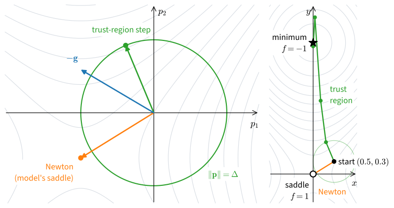
We solve the subproblem at \((0.5, 0.3)\) by hand, with \(\Delta = 0.5\). There \(\mathbf{g} = (0.5, -0.296)\) and \(\mathbf{B} = \mathrm{diag}(1, -0.955)\). Positive semidefiniteness of \(\mathbf{B} + \tau\mathbf{I}\) needs \(\tau \ge 0.955\), and the Newton point \(\tau = 0\) is excluded, so the step lies on the boundary. The equations are \((1 + \tau)p_1 = -0.5\) and \((\tau - 0.955)p_2 = 0.296\), with \(p_1^2 + p_2^2 = 0.25\). Their solution is \(\tau \approx 1.60\) and \(\mathbf{p} \approx (-0.19, 0.46)\). The new point \((0.31, 0.76)\) has \(f = 0.771\), down from \(1.080\). The model predicted a decrease of \(0.316\), the actual decrease is \(0.309\), and \(r = 0.98\), so the radius doubles. The step moves away from the saddle, along the direction of negative curvature, where the model falls, while the Newton step \((-0.5, -0.31)\) moves toward it.
One step by hand does not show where the rule leads. We implement the step by bisection on \(\tau\) and run six iterations, printing the iterate, \(f\), the step length, \(\tau\), the ratio, and the radius in force.
def tr_step(g, B, Delta):
    """Minimize g p + p B p / 2 over |p| <= Delta; return (p, tau)."""
    eig_min = np.linalg.eigvalsh(B).min()
    if eig_min > 0 and np.linalg.norm(np.linalg.solve(B, -g)) <= Delta:
        return np.linalg.solve(B, -g), 0.0     # Newton step fits: tau = 0
    lo = hi = max(0.0, -eig_min)
    hi += 1e3
    for _ in range(100):                       # bisection for |p(tau)| = Delta
        tau = (lo + hi) / 2
        p = np.linalg.solve(B + tau * np.eye(len(g)), -g)
        lo, hi = (tau, hi) if np.linalg.norm(p) > Delta else (lo, tau)
    return p, tau
x, Delta = np.array([0.5, 0.3]), 0.5
print(' k x f |p| tau r Delta')
for k in range(6):
g, B = grad_s(x), hess_s(x)
p, tau = tr_step(g, B, Delta)
r = (f_s(x) - f_s(x + p)) / -(g @ p + 0.5 * p @ B @ p)
print(f'{k:2d} ({x[0]:6.3f},{x[1]:6.3f}) {f_s(x):7.4f} '
f'{np.linalg.norm(p):6.3f} {tau:6.3f} {r:6.2f} {Delta:5.2f}')
if r > 0.1: # accept the step
x = x + p
if r < 0.25:
Delta /= 4 # poor prediction: shrink
elif r > 0.75 and np.linalg.norm(p) > 0.99 * Delta:
Delta *= 2 # good, and on the boundary
print(f'final x = ({x[0]:.4f}, {x[1]:.4f}), f = {f_s(x):.4f}') k x f |p| tau r Delta
0 ( 0.500, 0.300) 1.0803 0.500 1.596 0.98 0.50
1 ( 0.307, 0.761) 0.7711 1.000 1.419 0.87 1.00
2 ( 0.180, 1.753) -0.1652 2.000 0.311 0.41 2.00
3 ( 0.043, 3.749) -0.8205 0.696 0.000 0.88 2.00
4 ( 0.000, 3.054) -0.9962 0.088 0.000 1.00 2.00
5 ( 0.000, 3.142) -1.0000 0.000 0.000 1.00 2.00
final x = (0.0000, 3.1416), f = -1.0000The first row reproduces the hand computation. The radius grows from \(0.5\) to \(1\) and \(2\), and the third step, with ratio \(0.41\), is accepted without changing it. The fourth iterate, \((0.04, 3.75)\), lies in the region where the Hessian is positive definite. From there on the Newton step fits inside the ball and \(\tau = 0\), so the method has become Newton’s method. It converges quadratically to the minimum \((0, \pi)\), where \(f = -1\). Six iterations suffice. Figure 35.2.1 shows both runs.
The exact subproblem needs a factorization of \(\mathbf{B}_k + \tau\mathbf{I}\) for each trial \(\tau\). Large problems solve it approximately with Hessian–vector products, which cost about as much as a gradient (Section 34.5). Even so, neither BFGS nor a trust region replaces stochastic gradients on a large noisy loss.
The saddle of \(\tfrac12 x^2 + \cos y\) has now misled two methods: gradient descent stopped at it, and Newton’s method ran to it. A trust region escapes, but only by testing each model against the function. On some functions no such care is needed, because they have no saddle and no second basin, and every stationary point is the minimum. Which functions these are is the subject of Section 35.3.
35.2.4 Summary
Newton’s step minimizes the local quadratic model of \(f\). It solves a quadratic in one step whatever its condition number, and near a minimizer with a positive definite, Lipschitz-continuous Hessian it squares the error at every step. A step costs \(O(d^2)\) memory and \(O(d^3)\) time, which no network can afford, and the method runs to saddles as readily as to minima. BFGS rebuilds the inverse Hessian from the changes of the gradient along past steps, and on a quadratic in \(d\) dimensions it has rebuilt all of it after \(d\) steps. A trust region makes any quadratic model safe to use: it bounds the step, compares the predicted decrease with the actual one, and adjusts the bound accordingly.
35.2.5 Exercises
- Reparametrization and preconditioning. Let \(\mathbf{T}\) be an invertible matrix and \(h(\mathbf{y}) = f(\mathbf{T}\mathbf{y})\), so that \(\mathbf{x} = \mathbf{T}\mathbf{y}\) is a change of coordinates.
- Express \(\nabla h\) and \(\nabla^2 h\) through the derivatives of \(f\). Show that Newton’s iterates Equation 35.2.2 for \(h\), started at \(\mathbf{y}_0 = \mathbf{T}^{-1}\mathbf{x}_0\), satisfy \(\mathbf{y}_k = \mathbf{T}^{-1}\mathbf{x}_k\), where \(\mathbf{x}_k\) are Newton’s iterates for \(f\).
- Run gradient descent with step \(\eta\) on \(h\) and map every iterate back by \(\mathbf{x}_k = \mathbf{T}\mathbf{y}_k\). Show that the mapped iterates follow \(\mathbf{x}_{k+1} = \mathbf{x}_k - \eta\, \mathbf{P}^{-1} \nabla f(\mathbf{x}_k)\) for a positive definite matrix \(\mathbf{P}\), and find \(\mathbf{P}\). By problem 1b this direction is the steepest one in the norm \(\|\cdot\|_{\mathbf{P}}\). What is \(\|\mathbf{x}\|_{\mathbf{P}}\) in the coordinates \(\mathbf{y}\)?
- For \(f(\mathbf{x}) = \tfrac12\mathbf{x}^\top \mathbf{A}\,\mathbf{x}\) with \(\mathbf{A} = \mathrm{diag}(1, 1000)\), the \(\kappa = 1000\) quadratic of the Newton subsection, find a diagonal \(\mathbf{T}\) for which gradient descent on \(h\) with \(\eta = 1\) reaches the minimizer in one step. What does constructing such a \(\mathbf{T}\) require for a general positive definite \(\mathbf{A}\)?
- [code] BFGS on a quadratic. ● Let \(f(\mathbf{x}) = \tfrac12\mathbf{x}^\top\mathbf{A}\mathbf{x} - \mathbf{b}^\top\mathbf{x}\) with \(\mathbf{A}\) positive definite, and run BFGS Equation 35.2.5 with exact line searches from \(\mathbf{M}_0 = \mathbf{I}\).
- Show that an exact line search along \(\mathbf{p}_k\) gives \(\nabla f(\mathbf{x}_{k+1})^\top\mathbf{p}_k = 0\), and that \(\mathbf{y}_k = \mathbf{A}\mathbf{s}_k\).
- Show the hereditary property: if \(\mathbf{M}_k\mathbf{y}_j = \mathbf{s}_j\) for all \(j < k\) and the steps \(\mathbf{s}_0, \ldots, \mathbf{s}_{k-1}\), \(\mathbf{s}_k\) are \(\mathbf{A}\)-conjugate, then \(\mathbf{M}_{k+1}\mathbf{y}_j = \mathbf{s}_j\) for all \(j \le k\). (Hint: \(\mathbf{s}_j^\top\mathbf{y}_k = \mathbf{s}_j^\top\mathbf{A}\mathbf{s}_k = 0\) for \(j < k\).) Conclude that after \(d\) linearly independent steps \(\mathbf{M}_d\mathbf{A} = \mathbf{I}\).
- Run the BFGS loop of the text in \(d = 6\) dimensions, on a randomly rotated quadratic with eigenvalues from \(1\) to \(1000\). Print \(\max_{j \le k}\|\mathbf{M}_{k+1}\mathbf{y}_j - \mathbf{s}_j\|\) after each step, and confirm that it stays at rounding level and that \(\mathbf{M}_6 = \mathbf{A}^{-1}\). How far from the minimizer is gradient descent at its best fixed step after the same six gradients?
- The symmetric rank-one update \(\mathbf{M}_{k+1} = \mathbf{M}_k + \frac{(\mathbf{s} - \mathbf{M}_k\mathbf{y})(\mathbf{s} - \mathbf{M}_k\mathbf{y})^\top}{(\mathbf{s} - \mathbf{M}_k\mathbf{y})^\top\mathbf{y}}\) also satisfies the secant equation. Show by a \(2 \times 2\) example that it need not stay positive definite even when \(\mathbf{y}^\top\mathbf{s} > 0\), and say which of the two checks in the text fails for it.
- [code] Trust region at a saddle. ● Consider the model \(m(\mathbf{p}) = \mathbf{g}^\top\mathbf{p} + \tfrac12\mathbf{p}^\top\mathbf{B}\mathbf{p}\) with \(\mathbf{B} = \mathrm{diag}(1, -1)\) and \(\mathbf{g} = (\tfrac12, -\tfrac{3}{10})\).
- Show that \(m\) is unbounded below on \(\mathbb{R}^2\) and that the Newton point \(-\mathbf{B}^{-1}\mathbf{g} = (-\tfrac12, -\tfrac{3}{10})\) is a saddle of \(m\), not a minimum.
- Prove that the conditions of the subproblem proposition are sufficient: if \((\mathbf{B} + \tau\mathbf{I})\mathbf{p} = -\mathbf{g}\) with \(\tau \ge 0\), \(\mathbf{B} + \tau\mathbf{I} \succeq \mathbf{0}\), and \(\tau(\Delta - \|\mathbf{p}\|) = 0\), then every \(\|\mathbf{q}\| \le \Delta\) satisfies \(m(\mathbf{q}) \ge m(\mathbf{p}) + \tfrac{\tau}{2}(\|\mathbf{p}\|^2 - \|\mathbf{q}\|^2) \ge m(\mathbf{p})\). (Hint: expand \(m(\mathbf{q}) - m(\mathbf{p})\) around \(\mathbf{p}\) and use \(\mathbf{g} = -(\mathbf{B} + \tau\mathbf{I})\mathbf{p}\).)
- For \(\Delta = \tfrac12\) find \(\tau \ge 1\) by bisection on \(\|(\mathbf{B} + \tau\mathbf{I})^{-1}\mathbf{g}\| = \Delta\) (the answer is \(\tau \approx 1.65\), \(\mathbf{p} \approx (-0.19, 0.46)\)), and check that the step increases the coordinate with negative curvature while the Newton step decreases it.
- Replace \(\mathbf{g}\) by \((\tfrac12, 0)\). Show that \(\|(\mathbf{B} + \tau\mathbf{I})^{-1}\mathbf{g}\| = \tfrac12/(1 + \tau) \le \tfrac14\) for all \(\tau > 1\), so the boundary equation has no solution with \(\tau > 1\). Find the minimizers on the ball directly (they have \(\tau = 1\) and \(p_2 = \pm\sqrt{\Delta^2 - p_1^2}\)), and explain in one sentence what the ball does with a direction of negative curvature that the gradient does not see.