%matplotlib inline
from d2l import torch as d2l
import numpy as np
import time
import torch
from torch import nn
import torch.nn.functional as F12.5 DeltaNet and Corrective Memory Updates
The matrix memories in Section 12.4 update their state by addition. If a key is used more than once, its old and new values are superposed. Decay reduces old contributions by age, but cannot selectively replace the value associated with one key. DeltaNet addresses this problem by reading the current value before writing and storing only the correction (Schlag et al. 2021).
We first demonstrate the failure of additive writes on an overwrite task. We then derive the delta rule as one gradient step on a recall loss. Its non-diagonal transition requires a different chunked implementation, which we obtain from a triangular solve. Adding a decay gate gives Gated DeltaNet. The final section studies the additional state-tracking computations allowed by this transition.
Prerequisites: the matrix-state recurrence and its capacity law (Section 12.4, Equation 12.4.2), the chunked training schedule of Section 12.4.3, and the optimizer vocabulary of Chapter 9, in particular what “decoupled” weight decay means (Section 9.7). The training cells use a GPU when one is available; the identity checks run anywhere.
%matplotlib inline
from d2l import jax as d2l
from flax import nnx
import jax
from jax import numpy as jnp
import math
import numpy as np
import optax
import time
12.5.1 Limitations of Additive Writes
The capacity law of Section 12.4.1.1 describes crowding: storing more unit-norm pairs than the key dimension increases the interference term in Equation 12.4.2. There is a second failure, and it survives even when crowding is engineered away. Suppose the keys are few and mutually orthogonal, so that interference between different keys is exactly zero, but the stream keeps re-binding old keys to new values: today’s stock price under the same ticker, a variable reassigned in code, a character’s location as a story moves on. An additive memory handles re-binding badly, because addition cannot replace. After \(R\) writes to the same key \(\mathbf{k}\), the Hebbian state holds
\[ \mathbf{S}^\top \mathbf{k} = \mathbf{v}^{(1)} + \mathbf{v}^{(2)} + \cdots + \mathbf{v}^{(R)}: \]
all values written under \(\mathbf{k}\) are superposed, so the current value receives the same weight as the stale values. Retrieving the latest binding then requires distinguishing it among \(R\) candidates.
The corrective write repairs exactly this. Before writing, retrieve what the memory currently returns for the key; subtract it; then write. We first state the corrective update and derive it in the next section:
\[ \mathbf{S}_t = \mathbf{S}_{t-1} + \mathbf{k}_t \big(\mathbf{v}_t - \mathbf{S}_{t-1}^\top \mathbf{k}_t\big)^\top . \tag{12.5.1}\]
For a unit-norm key this replaces the stored value: reading back immediately after the write returns \(\mathbf{v}_t\) exactly, however many bindings preceded it. The experiment below makes the contrast quantitative. We hand-build both memories, with no training anywhere: \(8\) orthonormal keys in \(64\) dimensions (orthonormal so that cross-key interference is zero by construction and staleness is the only effect in view; unit-norm keys are also what Equation 12.4.2 assumes), values drawn from a codebook of \(32\) unit vectors, \(R\) writes per key in shuffled order. After the stream, we read every key and decode by the nearest codebook entry, scoring a hit only if the memory returns the key’s latest value.
rng = np.random.default_rng(0)

def overwrite_recall(rule, reps, num_keys=8, num_values=32, d=64, trials=200):
    """Recall of the latest value bound to each key, after R writes per key."""
    accs = []
    for R in reps:
        correct = total = 0
        for _ in range(trials):
            K = np.linalg.qr(rng.standard_normal((d, num_keys)))[0].T
            codebook = rng.standard_normal((num_values, d))
            codebook /= np.linalg.norm(codebook, axis=1, keepdims=True)
            writes = [(k, rng.integers(num_values)) for k in range(num_keys)
                      for _ in range(R)]
            rng.shuffle(writes)
            latest, S = {}, np.zeros((d, d))
            for kk, vv in writes:
                k, v = K[kk], codebook[vv]
                latest[kk] = vv
                if rule == 'delta':
                    S = S + np.outer(k, v - S.T @ k)   # Erase, then write
                else:
                    S = S + np.outer(k, v)             # Superimpose
            for kk in range(num_keys):
                read = S.T @ K[kk]
                correct += (codebook @ read).argmax() == latest[kk]
                total += 1
        accs.append(correct / total)
    return accs

reps = [1, 2, 4, 8]
hebbian, delta = (overwrite_recall(r, reps) for r in ('hebbian', 'delta'))
print(f"{'writes/key':>10} {'Hebbian':>9} {'delta':>7}")
for row in zip(reps, hebbian, delta):
    print('{:>10} {:>9.3f} {:>7.3f}'.format(*row))
assert min(delta) > 0.99, 'delta write must recall the latest value exactly'
assert hebbian[-1] < 0.4, 'Hebbian recall must collapse under overwrites'
d2l.plot(reps, [hebbian, delta], 'writes per key', 'recall of latest value',
         legend=['Hebbian write', 'delta write'], fmts=('-o', '-s'))
writes/key Hebbian delta
1 1.000 1.000
2 0.510 1.000
4 0.299 1.000
8 0.217 1.000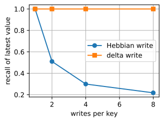
rng = np.random.default_rng(0)

def overwrite_recall(rule, reps, num_keys=8, num_values=32, d=64, trials=200):
    """Recall of the latest value bound to each key, after R writes per key."""
    accs = []
    for R in reps:
        correct = total = 0
        for _ in range(trials):
            K = np.linalg.qr(rng.standard_normal((d, num_keys)))[0].T
            codebook = rng.standard_normal((num_values, d))
            codebook /= np.linalg.norm(codebook, axis=1, keepdims=True)
            writes = [(k, rng.integers(num_values)) for k in range(num_keys)
                      for _ in range(R)]
            rng.shuffle(writes)
            latest, S = {}, np.zeros((d, d))
            for kk, vv in writes:
                k, v = K[kk], codebook[vv]
                latest[kk] = vv
                if rule == 'delta':
                    S = S + np.outer(k, v - S.T @ k)   # Erase, then write
                else:
                    S = S + np.outer(k, v)             # Superimpose
            for kk in range(num_keys):
                read = S.T @ K[kk]
                correct += (codebook @ read).argmax() == latest[kk]
                total += 1
        accs.append(correct / total)
    return accs

reps = [1, 2, 4, 8]
hebbian, delta = (overwrite_recall(r, reps) for r in ('hebbian', 'delta'))
print(f"{'writes/key':>10} {'Hebbian':>9} {'delta':>7}")
for row in zip(reps, hebbian, delta):
    print('{:>10} {:>9.3f} {:>7.3f}'.format(*row))
assert min(delta) > 0.99, 'delta write must recall the latest value exactly'
assert hebbian[-1] < 0.4, 'Hebbian recall must collapse under overwrites'
d2l.plot(reps, [hebbian, delta], 'writes per key', 'recall of latest value',
         legend=['Hebbian write', 'delta write'], fmts=('-o', '-s'))
writes/key Hebbian delta
1 1.000 1.000
2 0.510 1.000
4 0.299 1.000
8 0.217 1.000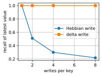
The additive memory collapses just as the superposition argument predicts: recall roughly halves by two writes per key and is down to about \(0.2\) by eight, close to picking at random among the values superposed on the key. The corrective write holds recall at \(1.000\) at every overwrite count, and not approximately: with \(\beta = 1\) and orthonormal keys, each write replaces the row it addresses and touches nothing else, so the last write always wins. Note what this experiment does not show: with only \(8\) orthogonal keys there is no crowding, so the decay ladder of Section 12.4.1.2 would not help here. Decay discounts by age; the failure is indexed by key.
12.5.1.1 End-to-End Training on the Overwrite Task
A trained model need not use its memory in the prescribed way above. Gradient descent might find an encoding that lets an additive memory avoid superposition, so we test this possibility with end-to-end training. The task generator below emits sequences with a write phase, \(R\) re-bindings of each of \(8\) keys in shuffled order, followed by a query phase asking for each key’s latest value; the model is trained end-to-end on cross-entropy over its answers.
def make_task(num_seqs, num_keys=8, num_values=16, R=4, seed=0):
    """R shuffled writes per key, then one query per key for its latest value."""
    task_rng = np.random.default_rng(seed)
    W = num_keys * R
    QUERY = num_values                     # A reserved "query" content token
    keys = np.zeros((num_seqs, W + num_keys), np.int64)
    vals = np.full((num_seqs, W + num_keys), QUERY, np.int64)
    tgt = np.full((num_seqs, W + num_keys), -1, np.int64)
    for b in range(num_seqs):
        ks = np.tile(np.arange(num_keys), R)
        vs = task_rng.integers(0, num_values, W)
        perm = task_rng.permutation(W)
        ks, vs = ks[perm], vs[perm]
        keys[b, :W], vals[b, :W] = ks, vs
        latest = {int(k): int(v) for k, v in zip(ks, vs)}
        qorder = task_rng.permutation(num_keys)
        keys[b, W:] = qorder
        tgt[b, W:] = [latest[int(k)] for k in qorder]
    return keys, vals, tgt                 # tgt = -1 outside the query phase
def make_task(num_seqs, num_keys=8, num_values=16, R=4, seed=0):
"""R shuffled writes per key, then one query per key for its latest value."""
task_rng = np.random.default_rng(seed)
W = num_keys * R
QUERY = num_values # A reserved "query" content token
keys = np.zeros((num_seqs, W + num_keys), np.int64)
vals = np.full((num_seqs, W + num_keys), QUERY, np.int64)
tgt = np.full((num_seqs, W + num_keys), -1, np.int64)
for b in range(num_seqs):
ks = np.tile(np.arange(num_keys), R)
vs = task_rng.integers(0, num_values, W)
perm = task_rng.permutation(W)
ks, vs = ks[perm], vs[perm]
keys[b, :W], vals[b, :W] = ks, vs
latest = {int(k): int(v) for k, v in zip(ks, vs)}
qorder = task_rng.permutation(num_keys)
keys[b, W:] = qorder
tgt[b, W:] = [latest[int(k)] for k in qorder]
return keys, vals, tgt # tgt = -1 outside the query phaseThe model is deliberately small: one matrix-memory layer, one MLP block, a classification head. One design decision is necessary for the comparison. The projections that produce \(\mathbf{q}_t\), \(\mathbf{k}_t\), and \(\beta_t\) form the write address, and they must see the key token alone, while the content \(\mathbf{v}_t\) must come from the value token alone. Give the address projection access to the value token and a trained Hebbian model escapes superposition entirely, by assigning every (key, value) pair its own private address so that no two writes ever collide; recall stops distinguishing the two rules. That escape is itself instructive, since superposition only binds when addresses are reused, but it dodges the question we are asking. Real linear-attention layers offer no such dodge at this task’s scale: \(\mathbf{q}\), \(\mathbf{k}\), \(\mathbf{v}\) are all projections of the same token embedding, so a model that answers “what is ticker X now” must address by the ticker. Our split enforces the shared-address regime we set out to measure.
class MemoryModel(nn.Module):
    """One matrix-memory layer plus an MLP block; address from the key only."""
    def __init__(self, num_keys, num_values, rule, d=64, d_head=48):
        super().__init__()
        self.rule = rule
        self.key_emb = nn.Embedding(num_keys, d)
        self.val_emb = nn.Embedding(num_values + 1, d)
        self.W_q = nn.Linear(d, d_head, bias=False)   # Address: from key only
        self.W_k = nn.Linear(d, d_head, bias=False)
        self.W_beta = nn.Linear(d, 1)
        self.W_v = nn.Linear(d, d_head, bias=False)   # Content: from value only
        self.W_o = nn.Linear(d_head, d, bias=False)
        self.ln1, self.ln2 = nn.LayerNorm(d), nn.LayerNorm(d)
        self.mlp = nn.Sequential(nn.Linear(d, 4 * d), nn.GELU(),
                                 nn.Linear(4 * d, d))
        self.head = nn.Linear(d, num_values)

    def forward(self, keys, vals):
        a, c = self.key_emb(keys), self.val_emb(vals)
        q = F.normalize(self.W_q(a), dim=-1)   # x / max(|x|, 1e-12)
        k = F.normalize(self.W_k(a), dim=-1)
        v, beta = self.W_v(c), torch.sigmoid(self.W_beta(a))
        B, T, d_head = v.shape
        S = v.new_zeros(B, d_head, d_head)
        outputs = []
        for t in range(T):
            k_t, v_t = k[:, t], v[:, t]
            if self.rule == 'delta':                   # Erase, then write
                u = beta[:, t] * (v_t - torch.einsum('bkv,bk->bv', S, k_t))
            else:                                      # Hebbian: superimpose
                u = v_t
            S = S + k_t[:, :, None] * u[:, None, :]
            outputs.append(torch.einsum('bkv,bk->bv', S, q[:, t]))
        h = a + c + self.W_o(torch.stack(outputs, 1))
        h = h + self.mlp(self.ln1(h))
        return self.head(self.ln2(h))
class MemoryModel(nnx.Module):
"""One matrix-memory layer plus an MLP block; address from the key only."""
def __init__(self, num_keys, num_values, rule, d=64, d_head=48, rngs=None):
rngs = nnx.Rngs(0) if rngs is None else rngs
self.rule = rule
self.key_emb = nnx.Embed(num_keys, d, rngs=rngs)
self.val_emb = nnx.Embed(num_values + 1, d, rngs=rngs)
self.W_q = nnx.Linear(d, d_head, use_bias=False, rngs=rngs)
self.W_k = nnx.Linear(d, d_head, use_bias=False, rngs=rngs)
self.W_beta = nnx.Linear(d, 1, rngs=rngs)
self.W_v = nnx.Linear(d, d_head, use_bias=False, rngs=rngs)
self.W_o = nnx.Linear(d_head, d, use_bias=False, rngs=rngs)
self.ln1, self.ln2 = (nnx.LayerNorm(d, rngs=rngs) for _ in range(2))
self.mlp_up = nnx.Linear(d, 4 * d, rngs=rngs)
self.mlp_down = nnx.Linear(4 * d, d, rngs=rngs)
self.head = nnx.Linear(d, num_values, rngs=rngs)
def __call__(self, keys, vals):
a, c = self.key_emb(keys), self.val_emb(vals)
norm = lambda x: x / jnp.maximum( # Same numerical contract as
jnp.linalg.norm(x, axis=-1, keepdims=True), 1e-12) # F.normalize
q, k = norm(self.W_q(a)), norm(self.W_k(a))
v, beta = self.W_v(c), jax.nn.sigmoid(self.W_beta(a))
B, T, d_head = v.shape
def step(S, qkvb):
q_t, k_t, v_t, b_t = qkvb
if self.rule == 'delta': # Erase, then write
u = b_t * (v_t - jnp.einsum('bkv,bk->bv', S, k_t))
else: # Hebbian: superimpose
u = v_t
S = S + k_t[:, :, None] * u[:, None, :]
return S, jnp.einsum('bkv,bk->bv', S, q_t)
xs = tuple(x.swapaxes(0, 1) for x in (q, k, v, beta))
_, outputs = jax.lax.scan(step, jnp.zeros((B, d_head, d_head)), xs)
h = a + c + self.W_o(outputs.swapaxes(0, 1))
h = h + self.mlp_down(jax.nn.gelu(self.mlp_up(self.ln1(h))))
return self.head(self.ln2(h))Training is a plain Adam loop, a couple of minutes in total for the whole sweep; the only asymmetry between the two runs is the single line that writes the state.
def train_recall(rule, R, num_keys=8, num_values=16, epochs=12,
                 num_train=4096, num_val=1024, batch_size=256):
    device = d2l.try_gpu()
    torch.manual_seed(0)
    data = [torch.tensor(x, device=device)
            for x in make_task(num_train, num_keys, num_values, R, seed=1)
            + make_task(num_val, num_keys, num_values, R, seed=2)]
    Xk, Xv, y, Vk, Vv, Vy = data
    model = MemoryModel(num_keys, num_values, rule).to(device)
    opt = torch.optim.Adam(model.parameters(), lr=3e-3)
    for epoch in range(epochs):
        for i in torch.randperm(num_train, device=device).split(batch_size):
            loss = F.cross_entropy(model(Xk[i], Xv[i]).reshape(-1, num_values),
                                   y[i].reshape(-1), ignore_index=-1)
            opt.zero_grad(); loss.backward(); opt.step()
    with torch.no_grad():
        pred, mask = model(Vk, Vv).argmax(-1), Vy != -1
        return float((pred[mask] == Vy[mask]).float().mean())

print(f"{'writes/key':>10} {'Hebbian':>9} {'delta':>7}")
final = {}
for R in [1, 2, 4, 6]:
    accs = [train_recall(rule, R) for rule in ('hebbian', 'delta')]
    final[R] = accs
    print(f'{R:>10} {accs[0]:>9.3f} {accs[1]:>7.3f}')
assert final[6][1] > 0.95, 'trained delta must keep near-perfect recall'
assert final[6][0] < 0.5, 'trained Hebbian must collapse under overwrites'
writes/key Hebbian delta
1 1.000 1.000
2 0.537 1.000
4 0.327 1.000
6 0.268 1.000def train_recall(rule, R, num_keys=8, num_values=16, epochs=12,
num_train=4096, num_val=1024, batch_size=256):
Xk, Xv, y = map(jnp.array, make_task(num_train, num_keys, num_values,
R, seed=1))
Vk, Vv, Vy = map(jnp.array, make_task(num_val, num_keys, num_values,
R, seed=2))
model = MemoryModel(num_keys, num_values, rule, rngs=nnx.Rngs(0))
optimizer = nnx.Optimizer(model, optax.adam(3e-3), wrt=nnx.Param)
@nnx.jit
def train_step(model, optimizer, keys, vals, tgt):
def loss_fn(model):
mask = tgt != -1
losses = optax.softmax_cross_entropy_with_integer_labels(
model(keys, vals), jnp.where(mask, tgt, 0))
return (losses * mask).sum() / mask.sum()
loss, grads = nnx.value_and_grad(loss_fn)(model)
optimizer.update(model, grads)
return loss
perm_rng = np.random.default_rng(0)
for epoch in range(epochs):
for i in np.split(perm_rng.permutation(num_train),
num_train // batch_size):
train_step(model, optimizer, Xk[i], Xv[i], y[i])
pred, mask = model(Vk, Vv).argmax(-1), Vy != -1
return float((jnp.where(mask, pred == Vy, False)).sum() / mask.sum())
print(f"{'writes/key':>10} {'Hebbian':>9} {'delta':>7}")
final = {}
for R in [1, 2, 4, 6]:
accs = [train_recall(rule, R) for rule in ('hebbian', 'delta')]
final[R] = accs
print(f'{R:>10} {accs[0]:>9.3f} {accs[1]:>7.3f}')
assert final[6][1] > 0.95, 'trained delta must keep near-perfect recall'
assert final[6][0] < 0.5, 'trained Hebbian must collapse under overwrites'writes/key Hebbian delta
1 1.000 1.000
2 0.531 1.000
4 0.327 1.000
6 0.265 1.000Training does not remove the additive write’s limitation in this setup. The trained Hebbian model follows the mechanistic result, reaching about \(0.5\) accuracy at two writes per key and roughly \(0.25\)–\(0.35\) by four to six, while the delta model learns a perfect overwriting memory and stays at \(1.000\) throughout. Both models have identical parameter counts and see identical data; the entire gap is the write rule. This synthetic failure has a production-scale echo: multi-query associative recall is essentially this task embedded in natural text, and it is the single synthetic that best predicts which efficient architectures close the quality gap to attention, a diagnosis Section 12.7 takes up in earnest.
12.5.2 The Delta Rule
Equation Equation 12.5.1 follows from a recall objective. When token \(t\) arrives, the memory should associate \(\mathbf{k}_t\) with \(\mathbf{v}_t\): the state \(\mathbf{S}\) should make the momentary recall loss
\[ \ell_t(\mathbf{S}) = \tfrac{1}{2}\, \big\| \mathbf{S}^\top \mathbf{k}_t - \mathbf{v}_t \big\|^2 \tag{12.5.2}\]
small: reading the memory at \(\mathbf{k}_t\) should return \(\mathbf{v}_t\). The gradient is
\[ \nabla_{\mathbf{S}}\, \ell_t(\mathbf{S}) = \mathbf{k}_t \big(\mathbf{S}^\top \mathbf{k}_t - \mathbf{v}_t\big)^\top, \tag{12.5.3}\]
an outer product of the key with the prediction error, what the memory answered minus what it should have answered. One step of gradient descent from \(\mathbf{S}_{t-1}\) with step size \(\beta_t\) is
\[ \mathbf{S}_t = \mathbf{S}_{t-1} - \beta_t\, \mathbf{k}_t \big(\mathbf{k}_t^\top \mathbf{S}_{t-1} - \mathbf{v}_t^\top\big), \tag{12.5.4}\]
which at \(\beta_t = 1\) is exactly the repair we used above. This is the delta rule, and it is old: it is the Widrow–Hoff least-mean-squares update of adaptive filtering (Widrow and Hoff 1960), rediscovered for fast-weight memories by Schlag et al. (2021) and made parallel, and thereby practical at modern scale, by Yang et al. (2024) . Multiplying out Equation 12.5.4 puts it in the transition-plus-write shape of Equation 12.4.1:
\[ \mathbf{S}_t = \big(\mathbf{I} - \beta_t\, \mathbf{k}_t \mathbf{k}_t^\top\big)\, \mathbf{S}_{t-1} + \beta_t\, \mathbf{k}_t \mathbf{v}_t^\top, \qquad \mathbf{o}_t = \mathbf{S}_t^\top \mathbf{q}_t . \tag{12.5.5}\]
The two forms emphasize different properties. The error form Equation 12.5.4 is the algorithm, four lines below, and the cheap one to run: two matrix–vector products per token, never a \(d_k \times d_k\) matrix in sight. The matrix form Equation 12.5.5 slots DeltaNet into the family template: the transition \(\mathbf{I} - \beta_t \mathbf{k}_t \mathbf{k}_t^\top\) is no longer diagonal, and the closing analysis examines the resulting dynamical expressivity. For a unit-norm key, the update interpolates: the value stored at \(\mathbf{k}_t\) moves to \((1 - \beta_t)\,\mathbf{v}_{\textrm{old}} + \beta_t\, \mathbf{v}_t\), so \(\beta_t\) is a learned write strength, produced by a sigmoid from the token, with \(\beta_t \approx 0\) preserving the old binding and \(\beta_t \approx 1\) replacing it, the input gate of Section 12.1 reborn as a per-token learning rate.
The learning-rate interpretation also relates the two write rules. Compare the Hebbian write under the same lens: adding \(\beta_t \mathbf{k}_t \mathbf{v}_t^\top\) is one gradient step on the alignment objective \(-\langle \mathbf{S}^\top \mathbf{k}_t, \mathbf{v}_t\rangle\), a loss that only ever asks the read-out to grow along \(\mathbf{v}_t\), never to be correct, so the updates pile up without feedback. The delta rule optimizes recall error and gets error-correction; linear attention optimizes alignment and gets superposition. Both are online learners running inside the forward pass, at test time, with no autograd involved; they differ only in their loss. This interpretation allows other optimizers in the inner loop. Section 12.6 develops that view and identifies the delta rule as one plain-SGD step on a least-squares loss.
One practical note before the code: all delta-rule implementations in this chapter \(L2\)-normalize keys (and queries), as shipped DeltaNet variants do. The reason is visible in Equation 12.5.5: along \(\mathbf{k}_t\) the transition scales the state by \(1 - \beta_t \|\mathbf{k}_t\|^2\), which for unnormalized keys and \(\beta_t\) near \(1\) can exceed \(1\) in magnitude and let repeated writes amplify the state geometrically. Unit keys pin that factor to \(1 - \beta_t \in (0, 1)\): stable, and cleanly interpretable as partial replacement.
def delta_recurrent(Q, K, V, beta):
    """The delta rule in the error form: read, subtract, write, read out."""
    S = Q.new_zeros(Q.shape[-1], V.shape[-1])
    outputs = []
    for t in range(Q.shape[0]):
        error = V[t] - S.T @ K[t]                # What the memory got wrong
        S = S + beta[t] * K[t][:, None] * error[None, :]
        outputs.append(S.T @ Q[t])
    return torch.stack(outputs)

def delta_recurrent_matrix(Q, K, V, beta):
    """The same update as transition-then-write, for the family template."""
    S = Q.new_zeros(Q.shape[-1], V.shape[-1])
    I = torch.eye(Q.shape[-1], device=Q.device)
    outputs = []
    for t in range(Q.shape[0]):
        S = (I - beta[t] * torch.outer(K[t], K[t])) @ S \
            + beta[t] * torch.outer(K[t], V[t])
        outputs.append(S.T @ Q[t])
    return torch.stack(outputs)

torch.manual_seed(0)
d_k, d_v, T = 64, 64, 512
Q, K, V = (torch.randn(T, d, device=d2l.try_gpu()) for d in (d_k, d_k, d_v))
K = F.normalize(K, dim=-1)                       # Unit-norm keys, throughout
beta = torch.sigmoid(torch.randn(T, device=d2l.try_gpu()))
y_delta = delta_recurrent(Q, K, V, beta)
err = (y_delta - delta_recurrent_matrix(Q, K, V, beta)).abs().max() \
    / y_delta.abs().max()
print(f'error form vs matrix form: relative deviation {float(err):.2e}')
assert err < 1e-5                  # One rule, two readings
error form vs matrix form: relative deviation 1.88e-06def delta_recurrent(Q, K, V, beta):
"""The delta rule in the error form: read, subtract, write, read out."""
def step(S, qkvb):
q, k, v, b = qkvb
error = v - S.T @ k # What the memory got wrong
S = S + b * k[:, None] * error[None, :]
return S, S.T @ q
S0 = jnp.zeros((Q.shape[-1], V.shape[-1]))
return jax.lax.scan(step, S0, (Q, K, V, beta))[1]
def delta_recurrent_matrix(Q, K, V, beta):
"""The same update as transition-then-write, for the family template."""
def step(S, qkvb):
q, k, v, b = qkvb
S = (jnp.eye(len(k)) - b * jnp.outer(k, k)) @ S + b * jnp.outer(k, v)
return S, S.T @ q
S0 = jnp.zeros((Q.shape[-1], V.shape[-1]))
return jax.lax.scan(step, S0, (Q, K, V, beta))[1]
d_k, d_v, T = 64, 64, 512
rng_keys = jax.random.split(jax.random.key(0), 4)
Q, K, V = (jax.random.normal(k, (T, d))
for k, d in zip(rng_keys, (d_k, d_k, d_v)))
K = K / jnp.maximum(jnp.linalg.norm(K, axis=-1, keepdims=True),
1e-12) # Unit keys; F.normalize contract
beta = jax.nn.sigmoid(jax.random.normal(rng_keys[3], (T,)))
with jax.default_matmul_precision('highest'):
y_delta = delta_recurrent(Q, K, V, beta)
err = jnp.abs(y_delta - delta_recurrent_matrix(Q, K, V, beta)).max() \
/ jnp.abs(y_delta).max()
print(f'error form vs matrix form: relative deviation {float(err):.2e}')
assert err < 1e-5 # One rule, two readingserror form vs matrix form: relative deviation 1.38e-0612.5.3 Chunked Training with the WY Representation
The recurrence above is fine for generation, one token, constant memory, but training wants the whole sequence at once, and here DeltaNet is more involved than the scalar transition in Section 12.4. The chunked schedule of Section 12.4.3 leaned on the transition being a scalar: products of decays collapse into segsum, an elementwise log-space cumulative sum. DeltaNet’s transitions are the matrices \(\mathbf{I} - \beta_t \mathbf{k}_t \mathbf{k}_t^\top\), and a product of those is not elementwise anything; materializing the cumulative products would cost a \(d_k \times d_k\) matrix multiply per token, exactly the parallelism-killing serial chain we are trying to avoid.
The shared structure of the updates provides a parallel formulation. Write the state at the end of a chunk of \(C\) tokens, entered with state \(\mathbf{S}\), in the error form: each token contributes a rank-one write \(\mathbf{k}_t \mathbf{u}_t^\top\) with update vector \(\mathbf{u}_t = \beta_t (\mathbf{v}_t - \mathbf{S}_{t-1}^\top \mathbf{k}_t)\). The trouble is that \(\mathbf{u}_t\) depends on \(\mathbf{S}_{t-1}\), which contains every earlier update in the chunk. Substituting \(\mathbf{S}_{t-1} = \mathbf{S} + \sum_{s<t} \mathbf{k}_s \mathbf{u}_s^\top\) makes the dependency explicit:
\[ \mathbf{u}_t = \beta_t \big(\mathbf{v}_t - \mathbf{S}^\top \mathbf{k}_t\big) - \beta_t \sum_{s<t} (\mathbf{k}_s^\top \mathbf{k}_t)\, \mathbf{u}_s . \tag{12.5.6}\]
The updates couple only through the scalars \(\mathbf{k}_s^\top \mathbf{k}_t\), key overlaps we can compute for the whole chunk in one matmul. Stack the \(\mathbf{u}_t^\top\) as the rows of \(\mathbf{U} \in \mathbb{R}^{C \times d_v}\) and Equation 12.5.6 becomes a unit lower triangular linear system,
\[ (\mathbf{I} + \mathbf{A})\, \mathbf{U} = \mathrm{diag}(\boldsymbol{\beta}) \big(\mathbf{V} - \mathbf{K}\mathbf{S}\big), \qquad A_{ts} = \beta_t\, (\mathbf{k}_t^\top \mathbf{k}_s)\; \textrm{for } s < t, \textrm{ else } 0, \tag{12.5.7}\]
solved by forward substitution, one triangular solve per chunk. The widths matter in the accounting: forming the coupling matrix \(\mathbf{A}\) is a \(\mathcal{O}(C^2 d_k)\) matmul, and the forward substitution costs \(\mathcal{O}(C^2 d_v)\), its right-hand side having \(d_v\) columns — the same order as the attention-shaped matmuls around it, not free. (Numerical linear algebra veterans will recognize the maneuver: expressing a product of rank-one modifications, \(\prod_t (\mathbf{I} - \beta_t \mathbf{k}_t \mathbf{k}_t^\top)\), through a compact coupling matrix is the classical WY representation of products of Householder-like transformations, which is why the fast form of DeltaNet goes by that name (Yang et al. 2024).) With \(\mathbf{U}\) in hand, everything else is the familiar two-piece schedule of Section 12.4.3: outputs are the read of the inherited state plus a causal attention-shaped matmul against the chunk’s own updates, \(\mathbf{Y} = \mathbf{Q}\mathbf{S} + \mathrm{tril}(\mathbf{Q}\mathbf{K}^\top)\,\mathbf{U}\), and the state advances by \(\mathbf{S} \leftarrow \mathbf{S} + \mathbf{K}^\top \mathbf{U}\). The resulting schedule uses attention within each chunk, recurrence across chunks, and one triangular solve:
def delta_chunked(Q, K, V, beta, chunk_size=64):
    """Chunked WY form: one triangular solve per chunk, a state across chunks."""
    C = chunk_size
    Qc, Kc = Q.view(-1, C, Q.shape[-1]), K.view(-1, C, K.shape[-1])
    Vc, bc = V.view(-1, C, V.shape[-1]), beta.view(-1, C)
    I = torch.eye(C, device=Q.device)
    A = torch.tril(bc[:, :, None] * (Kc @ Kc.transpose(-1, -2)), -1)
    S = Q.new_zeros(Q.shape[-1], V.shape[-1])
    Y = []
    for c in range(Q.shape[0] // C):       # T/C boundary steps
        U = torch.linalg.solve_triangular(  # Solve against the actual RHS:
            I + A[c], bc[c][:, None] * (Vc[c] - Kc[c] @ S),
            upper=False, unitriangular=True)  # never form the inverse
        Y.append(Qc[c] @ S + torch.tril(Qc[c] @ Kc[c].T) @ U)
        S = S + Kc[c].T @ U
    return torch.cat(Y)

for chunk_size in [16, 64, 256]:
    err = (delta_chunked(Q, K, V, beta, chunk_size) - y_delta).abs().max() \
        / y_delta.abs().max()
    print(f'chunk size {chunk_size:4d}: relative deviation {float(err):.2e}')
    assert err < 1e-3                      # Chunked == recurrence
chunk size 16: relative deviation 3.00e-07
chunk size 64: relative deviation 4.03e-07
chunk size 256: relative deviation 3.63e-07def delta_chunked(Q, K, V, beta, chunk_size=64):
"""Chunked WY form: one triangular solve per chunk, a state across chunks."""
C = chunk_size
Qc, Kc = Q.reshape(-1, C, Q.shape[-1]), K.reshape(-1, C, K.shape[-1])
Vc, bc = V.reshape(-1, C, V.shape[-1]), beta.reshape(-1, C)
I = jnp.eye(C)
A = jnp.tril(bc[:, :, None] * (Kc @ Kc.transpose(0, 2, 1)), -1)
def boundary(S, chunk): # T/C boundary steps
Qb, Kb, Vb, bb, Ab = chunk
U = jax.scipy.linalg.solve_triangular( # Solve against the actual
I + Ab, bb[:, None] * (Vb - Kb @ S), # RHS: never form the
lower=True, unit_diagonal=True) # inverse
Y = Qb @ S + jnp.tril(Qb @ Kb.T) @ U
return S + Kb.T @ U, Y
S0 = jnp.zeros((Q.shape[-1], V.shape[-1]))
_, Y = jax.lax.scan(boundary, S0, (Qc, Kc, Vc, bc, A))
return Y.reshape(len(Q), -1)
with jax.default_matmul_precision('highest'):
for chunk_size in [16, 64, 256]:
err = jnp.abs(delta_chunked(Q, K, V, beta, chunk_size)
- y_delta).max() / jnp.abs(y_delta).max()
print(f'chunk size {chunk_size:4d}: relative deviation {float(err):.2e}')
assert err < 1e-3 # Chunked == recurrencechunk size 16: relative deviation 3.46e-07
chunk size 64: relative deviation 4.32e-07
chunk size 256: relative deviation 4.76e-07Agreement to floating-point rounding at every chunk size: the triangular solve is the sequential recurrence, reorganized. The cost accounting matches the scalar-decay case of Section 12.4.3 almost line for line, diagonal blocks of attention-shaped matmuls, a state carried across \(T/C\) boundaries, with one addition: the per-chunk unit-triangular solve for \(\mathbf{U}\), taken directly against the chunk’s right-hand side \(\mathrm{diag}(\boldsymbol{\beta})(\mathbf{V} - \mathbf{K}
\mathbf{S})\) at \(\mathcal{O}(C^2 d_v)\). Materializing \((\mathbf{I} + \mathbf{A})^{-1}\) first and multiplying would give the same answer at \(\mathcal{O}(C^3)\) plus a stored matrix nobody needs; solving against the right-hand side is both the cheaper and the more numerically well-behaved habit. This implementation omits head batching, gating, tensor-core-aware tiling, and low-precision safeguards used by production kernels. The open-source flash-linear-attention library implements these extensions and serves as a reference for most models in this family.
12.5.4 Gating and the Modern Cell
DeltaNet edits the row it writes; every other row it preserves exactly, since the transition acts as the identity off \(\mathbf{k}_t\). This produces the complementary limitation to pure decay: a pure-decay model forgets all directions, whereas a pure-delta model forgets a direction only when a new write overlaps its key. Values associated with keys that are never queried again therefore remain in the state and contribute to crowding. The modern cell therefore uses both knobs, a scalar decay and the delta write (Yang et al. 2025):
\[ \mathbf{S}_t = \alpha_t \big(\mathbf{I} - \beta_t\, \mathbf{k}_t \mathbf{k}_t^\top\big)\, \mathbf{S}_{t-1} + \beta_t\, \mathbf{k}_t \mathbf{v}_t^\top, \qquad \alpha_t \in (0, 1),\; \beta_t \in (0, 1). \tag{12.5.8}\]
This is Gated DeltaNet, and the design has a familiar shape. In the online-learner reading, \(\beta_t\) is a learning rate and \(\alpha_t\) is weight decay, and Equation 12.5.8 applies them decoupled: the decay shrinks the whole state first, and the gradient step is taken at its own, independently controlled strength, the same fix that distinguishes AdamW from Adam-with-\(L2\) in Section 9.7. The analogy applies only to the separation of the two rates: the model can set forgetting and learning independently at each token. There are no gradient moments or bias corrections in Equation 12.5.8, only AdamW’s decoupling of decay from step. On the ladder of Figure 12.4.1, this is the dashed rung, one step past the diagonal: decay everywhere, plus a rank-one edit.
Strike the erase term \(-\alpha_t \beta_t \mathbf{k}_t \mathbf{k}_t^\top \mathbf{S}_{t-1}\), keeping decay and write, and you are back at Mamba-2’s row of Table 12.4.1; set \(\alpha_t = 1\) and you have pure DeltaNet, so this one cell holds both parents of the family in two sigmoids. It is also, at the time of writing, the family’s production representative: Qwen3-Next interleaves Gated DeltaNet with a few full-attention layers, and Kimi Linear’s KDA layer is a Gated DeltaNet whose forgetting is refined from a scalar to a per-channel diagonal (Kimi Team 2025), with the ratio of recurrent to attention layers a design axis Section 12.7 will price.
12.5.4.1 A Language Model
Every architecture this chapter takes seriously must face the scoreboard of Section 12.3.3.1. The block below wraps the gated delta recurrence with the standard components used by the preceding language models: pre-norm residuals, two heads with per-head states (\(\mathbf{q}, \mathbf{k}\) normalized per head, matching the unit-key convention above), an output RMSNorm and a SiLU gate on the read-out (this family normalizes the output rather than carrying a normalizer state, as discussed in Section 12.4), and a small MLP for channel mixing, since the memory read is linear across channels. We bias \(\alpha_t\) toward \(1\) at initialization so an untrained model retains by default, the same open-the-forget-gate trick used since the LSTM. For training we keep the transparent token loop, fast enough at \(32\) steps per window; the WY form above is how the same model would train at real sequence lengths.
class GatedDeltaNetBlock(nn.Module):
    """Pre-norm residual: gated delta-rule memory, then a position-wise MLP."""
    def __init__(self, num_hiddens, num_heads=2, dropout=0):
        super().__init__()
        d, self.num_heads = num_hiddens, num_heads
        self.d_head = d // num_heads
        self.ln1, self.ln2 = nn.LayerNorm(d), nn.LayerNorm(d)
        self.W_qkv = nn.Linear(d, 3 * d, bias=False)
        self.W_ab = nn.Linear(d, 2 * num_heads)   # alpha, beta per head
        self.norm = nn.RMSNorm(self.d_head)
        self.W_gate = nn.Linear(d, d)
        self.W_o = nn.Linear(d, d, bias=False)
        self.mlp = nn.Sequential(nn.Linear(d, 2 * d), nn.GELU(),
                                 nn.Linear(2 * d, d))
        self.drop = nn.Dropout(dropout)
        nn.init.constant_(self.W_ab.bias[:num_heads], 2.0)  # Retain by default

    def forward(self, X):                    # (num_steps, batch, num_hiddens)
        T, B, d = X.shape
        h = self.ln1(X)
        q, k, v = self.W_qkv(h).reshape(T, B, self.num_heads, 3,
                                        self.d_head).unbind(3)
        q, k = F.normalize(q, dim=-1), F.normalize(k, dim=-1)
        alpha, beta = torch.sigmoid(self.W_ab(h)).chunk(2, -1)
        S = X.new_zeros(B, self.num_heads, self.d_head, self.d_head)
        outputs = []
        for t in range(T):                   # Decay, then erase-and-write
            S = alpha[t].unsqueeze(-1).unsqueeze(-1) * S
            error = v[t] - torch.einsum('bhkv,bhk->bhv', S, k[t])
            S = S + (beta[t].unsqueeze(-1) * k[t]).unsqueeze(-1) \
                * error.unsqueeze(-2)
            outputs.append(torch.einsum('bhkv,bhk->bhv', S, q[t]))
        o = self.norm(torch.stack(outputs))  # (T, B, heads, d_head)
        o = (o * F.silu(self.W_gate(h)).reshape(T, B, self.num_heads,
                                                self.d_head)).reshape(T, B, d)
        X = X + self.drop(self.W_o(o))
        return X + self.drop(self.mlp(self.ln2(X)))

class GatedDeltaNet(d2l.Module):
    """A stack of blocks with the recurrent-cell interface."""
    def __init__(self, num_inputs, num_blocks=2, num_heads=2, dropout=0):
        super().__init__()
        self.save_hyperparameters()
        self.num_hiddens = num_inputs
        self.blocks = nn.Sequential(*[
            GatedDeltaNetBlock(num_inputs, num_heads, dropout)
            for _ in range(num_blocks)])
        self.ln = nn.LayerNorm(num_inputs)

    def forward(self, X, state=None):
        return self.ln(self.blocks(X)), None
class GatedDeltaNetBlock(nnx.Module):
"""Pre-norm residual: gated delta-rule memory, then a position-wise MLP."""
def __init__(self, num_hiddens, num_heads=2, dropout=0, rngs=None):
rngs = nnx.Rngs(0) if rngs is None else rngs
d, self.num_heads = num_hiddens, num_heads
self.d_head = d // num_heads
self.ln1 = nnx.LayerNorm(d, rngs=rngs)
self.ln2 = nnx.LayerNorm(d, rngs=rngs)
self.W_qkv = nnx.Linear(d, 3 * d, use_bias=False, rngs=rngs)
self.W_ab = nnx.Linear( # alpha, beta per head
d, 2 * num_heads, rngs=rngs, # Retain by default:
bias_init=lambda key, shape, dtype: jnp.concatenate(
[2.0 * jnp.ones(num_heads), jnp.zeros(num_heads)]))
self.norm = nnx.RMSNorm(self.d_head, rngs=rngs)
self.W_gate = nnx.Linear(d, d, rngs=rngs)
self.W_o = nnx.Linear(d, d, use_bias=False, rngs=rngs)
self.mlp_up = nnx.Linear(d, 2 * d, rngs=rngs)
self.mlp_down = nnx.Linear(2 * d, d, rngs=rngs)
self.drop = nnx.Dropout(dropout, rngs=rngs)
def __call__(self, X): # (num_steps, batch, num_hiddens)
T, B, d = X.shape
h = self.ln1(X)
qkv = self.W_qkv(h).reshape(T, B, self.num_heads, 3, self.d_head)
unit = lambda x: x / jnp.maximum( # Same numerical contract as
jnp.linalg.norm(x, axis=-1, keepdims=True), 1e-12) # F.normalize
q, k, v = unit(qkv[..., 0, :]), unit(qkv[..., 1, :]), qkv[..., 2, :]
ab = jax.nn.sigmoid(self.W_ab(h))
alpha, beta = ab[..., :self.num_heads], ab[..., self.num_heads:]
def step(S, xs): # Decay, then erase-and-write
q_t, k_t, v_t, a_t, b_t = xs
S = a_t[..., None, None] * S
error = v_t - jnp.einsum('bhkv,bhk->bhv', S, k_t)
S = S + (b_t[..., None] * k_t)[..., None] * error[..., None, :]
return S, jnp.einsum('bhkv,bhk->bhv', S, q_t)
S0 = jnp.zeros((B, self.num_heads, self.d_head, self.d_head))
_, o = jax.lax.scan(step, S0, (q, k, v, alpha, beta))
o = self.norm(o) # (T, B, heads, d_head)
o = (o * jax.nn.silu(self.W_gate(h)).reshape(
T, B, self.num_heads, self.d_head)).reshape(T, B, d)
X = X + self.drop(self.W_o(o))
return X + self.drop(self.mlp_down(jax.nn.gelu(self.mlp_up(
self.ln2(X)))))
class GatedDeltaNet(nnx.Module):
"""A stack of blocks with the recurrent-cell interface."""
def __init__(self, num_inputs, num_blocks=2, num_heads=2, dropout=0,
rngs=None):
rngs = nnx.Rngs(0) if rngs is None else rngs
self.num_inputs = self.num_hiddens = num_inputs
self.blocks = nnx.Sequential(*[
GatedDeltaNetBlock(num_inputs, num_heads, dropout, rngs=rngs)
for _ in range(num_blocks)])
self.ln = nnx.LayerNorm(num_inputs, rngs=rngs)
def __call__(self, X, state=None):
return self.ln(self.blocks(X)), NoneThe training recipe is copied from the Mamba row of Section 12.3.3.1, The Time Machine under the BPE tokenizer, 50,000 windows of 32 tokens, ten epochs, Adam at a gentle learning rate with dropout on the residual branches, because this model shares Mamba’s appetite for memorizing a small corpus. d2l.RNNLM supplies embedding and head unchanged.
class GatedDeltaNetLM(d2l.RNNLM):
    def configure_optimizers(self):
        return torch.optim.Adam(self.parameters(), lr=self.lr)

data = d2l.TimeMachine(batch_size=1024, num_steps=32,
                       num_train=50000, num_val=5000)
torch.manual_seed(0)
model = GatedDeltaNetLM(GatedDeltaNet(num_inputs=128, dropout=0.3),
                        vocab_size=len(data.vocab), lr=3e-4)
trainer = d2l.Trainer(max_epochs=10, gradient_clip_val=1, num_gpus=1)
model.board.yscale = 'log'
start = time.time()
trainer.fit(model, data)
secs = (time.time() - start) / 10
ppl = float(model.board.data['val_ppl'][-1].y)
params = sum(p.numel() for p in model.parameters() if p.requires_grad)
print(f'{"model":>15} {"val ppl":>8} {"params":>9} {"s/epoch":>8}')
print(f'{"Gated DeltaNet":>15} {ppl:>8.1f} {params:>9,} {secs:>8.1f}')
model val ppl params s/epoch
Gated DeltaNet 83.7 562,315 5.4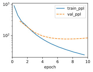
class GatedDeltaNetLM(d2l.RNNLM):
    def configure_optimizers(self):
        return optax.adam(self.lr)

data = d2l.TimeMachine(batch_size=1024, num_steps=32,
                       num_train=50000, num_val=5000)
model = GatedDeltaNetLM(GatedDeltaNet(num_inputs=128, dropout=0.3),
                        vocab_size=len(data.vocab), lr=3e-4)
trainer = d2l.Trainer(max_epochs=10, gradient_clip_val=1, num_gpus=1)
model.board.yscale = 'log'
start = time.time()
trainer.fit(model, data)
secs = (time.time() - start) / 10

def val_ppl(model):
    model = nnx.view(model, deterministic=True, use_running_average=True,
                     raise_if_not_found=False)  # Dropout off for evaluation
    total_loss = num_tokens = 0
    for X_val, y_val in data.val_dataloader():
        losses = model.loss(model(X_val), y_val, averaged=False)
        total_loss += float(losses.sum())
        num_tokens += losses.size
    return math.exp(total_loss / num_tokens)

params = sum(p.size for p in jax.tree.leaves(nnx.state(model, nnx.Param)))
print(f'{"model":>15} {"val ppl":>8} {"params":>9} {"s/epoch":>8}')
print(f'{"Gated DeltaNet":>15} {val_ppl(model):>8.1f} {params:>9,} '
      f'{secs:>8.1f}')
model val ppl params s/epoch
Gated DeltaNet 74.5 562,315 4.4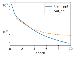
In our runs the row lands in the same band as the strongest models of Section 12.3.3.1, mid-seventies to mid-eighties of validation perplexity depending on framework and seed, at a comparable parameter count, without touching that scoreboard’s recipe beyond what its Mamba row already used. At this corpus size that is all the claim we make: the gated delta cell is competitive as a language model while carrying the overwriting memory the additive family lacks. At 1.3B parameters and real token budgets, the published version of the same comparison has Gated DeltaNet beating Mamba-2 and DeltaNet individually on perplexity and recall-heavy evaluations (Yang et al. 2025), with the two mechanisms’ contributions cleanly ablatable: decay without delta (Mamba-2) trails on recall, delta without decay (DeltaNet) trails on modeling; the cell that does both leads on both.
12.5.4.2 The Generalized Delta Rule
Once the transition is allowed to be “diagonal plus rank-one”, Gated DeltaNet’s \(\alpha_t (\mathbf{I} - \beta_t \mathbf{k}_t \mathbf{k}_t^\top)\) is one point in a small design space, and the other prominent occupant arrived from the RNN lineage. RWKV-7 (Peng et al. 2025) decouples every role the delta rule ties together:
\[ \mathbf{S}_t = \big(\mathrm{diag}(\mathbf{w}_t) - (\mathbf{a}_t \odot \hat{\boldsymbol{\kappa}}_t)\, \hat{\boldsymbol{\kappa}}_t^\top\big)\, \mathbf{S}_{t-1} + \tilde{\mathbf{k}}_t \mathbf{v}_t^\top . \tag{12.5.9}\]
Here \(\mathbf{w}_t\) is a per-channel decay (the GLA rung of the ladder, where Gated DeltaNet keeps a scalar), the unit vector \(\hat{\boldsymbol{\kappa}}_t\) is a removal key that need not equal the write key \(\tilde{\mathbf{k}}_t\), and \(\mathbf{a}_t\) is a per-channel in-context learning rate. The model can erase one address while writing another, decay each coordinate at its own rate, and modulate the erase per channel. Set all three to the delta-rule tying (no decay, removal key equal to write key, uniform rate \(\beta\)) and the update collapses back to DeltaNet; the cell below asserts as much, which is also a useful check that Equation 12.5.9 (stated here in this chapter’s convention; see the margin note of Section 12.4.4) is the update we claim it is. We reimplement the step from the paper’s equations; the reference code, released under Apache 2.0 alongside a line-by-line explainer, matches it in about ten lines.
def rwkv7_step(S, w, kappa, a, k_tilde, v):
    """One RWKV-7 state update: per-channel decay, rank-1 erase, write."""
    erase = (a * kappa)[:, None] * (kappa @ S)[None, :]
    return w[:, None] * S - erase + np.outer(k_tilde, v)

d = 8
S = rng.standard_normal((d, d))
k, v = rng.standard_normal(d), rng.standard_normal(d)
k /= np.linalg.norm(k)
b = 0.7                                    # One write strength for every role
S_rwkv = rwkv7_step(S, np.ones(d), k, b * np.ones(d), b * k, v)
S_delta = (np.eye(d) - b * np.outer(k, k)) @ S + b * np.outer(k, v)
print(f'RWKV-7, delta-rule setting: max deviation '
      f'{np.abs(S_rwkv - S_delta).max():.2e}')
assert np.abs(S_rwkv - S_delta).max() < 1e-12
RWKV-7, delta-rule setting: max deviation 4.44e-16def rwkv7_step(S, w, kappa, a, k_tilde, v):
"""One RWKV-7 state update: per-channel decay, rank-1 erase, write."""
erase = (a * kappa)[:, None] * (kappa @ S)[None, :]
return w[:, None] * S - erase + np.outer(k_tilde, v)
d = 8
S = rng.standard_normal((d, d))
k, v = rng.standard_normal(d), rng.standard_normal(d)
k /= np.linalg.norm(k)
b = 0.7 # One write strength for every role
S_rwkv = rwkv7_step(S, np.ones(d), k, b * np.ones(d), b * k, v)
S_delta = (np.eye(d) - b * np.outer(k, k)) @ S + b * np.outer(k, v)
print(f'RWKV-7, delta-rule setting: max deviation '
f'{np.abs(S_rwkv - S_delta).max():.2e}')
assert np.abs(S_rwkv - S_delta).max() < 1e-12RWKV-7, delta-rule setting: max deviation 4.44e-16Two shipped families sit within a couple of parameter-tying choices of Equation 12.5.8, Gated DeltaNet in Qwen3-Next and KDA in Kimi Linear (Kimi Team 2025), and so does RWKV-7’s own model line. What in Section 12.4 was a table of independent-looking models has become, one write rule later, a family with two parents: choose the decay structure (scalar, diagonal), choose the write rule (additive, delta, generalized delta), and the model largely follows.
12.5.5 Computational Properties of the Transition
The same transition also determines which state dynamics the model can represent. Look at Equation 12.5.5 once more, not as a write to a memory but as a linear dynamical system: DeltaNet’s transition \(\mathbf{I} - \beta_t \mathbf{k}_t \mathbf{k}_t^\top\) is the first transition in this chapter that is not diagonal. Its spectrum is easy to read off: eigenvalue \(1 - \beta_t\) along \(\mathbf{k}_t\), eigenvalue \(1\) on the orthogonal complement. Every transition in Table 12.4.1, by contrast, has non-negative eigenvalues: decays in \((0, 1)\) can shrink a state coordinate, but can never flip its sign. Does that limit what these models can compute, as opposed to remember?
Parity provides a minimal example of this limitation. Read a bit stream and answer whether the number of ones so far is even. A one-dimensional recurrence solves it exactly: multiply the state by \(-1\) on every one-bit, and the sign of the state is the answer. But that solution needs a transition value of \(-1\). A model whose transitions are confined to \([0, 1]\) can represent parity of the count only through precision tricks, and finite-precision analysis says essentially not at all (Grazzi et al. 2025). The experiment below isolates this boundary and depends on two design choices. First, the recurrence is purely multiplicative, \(\mathbf{h}_t = \mathbf{a}_t \odot \mathbf{h}_{t-1}\) from a nonzero learned \(\mathbf{h}_0\), with no input drive: parity lives in sign flips, and an additive drive hands the model a way to bury the flip mechanism in magnitudes, which in our trials left both variants at chance. Second, the sequences are short, training at \(T \le 24\): the point is the eigenvalue range, not long-horizon optimization, which fails for its own reasons soon enough. The two models below differ in one activation: the per-channel transition \(\mathbf{a}_t\) comes from a sigmoid, range \((0, 1)\), or from a tanh, range \((-1, 1)\). Because success at the edge of trainability is seed-dependent, we train three seeds per configuration and report each.
class MultiplicativeRNN(nn.Module):
    """h_t = a_t * h_{t-1}, elementwise; nonzero h_0; no input drive."""
    def __init__(self, act, num_hiddens=8):
        super().__init__()
        self.emb = nn.Embedding(2, num_hiddens)
        self.W_a = nn.Linear(num_hiddens, num_hiddens)
        self.h0 = nn.Parameter(torch.ones(num_hiddens)
                               + 0.1 * torch.randn(num_hiddens))
        self.head = nn.Linear(num_hiddens, 2)
        self.act = act

    def forward(self, X):
        a = self.act(self.W_a(self.emb(X)))      # (batch, T, num_hiddens)
        h = self.h0.expand(X.shape[0], -1)
        for t in range(X.shape[1]):
            h = a[:, t] * h
        return self.head(h)

def train_parity(act, T, seed, num_train=8192, num_val=2048, epochs=60,
                 batch_size=256):
    torch.manual_seed(seed)
    data_rng = np.random.default_rng(1)
    X = data_rng.integers(0, 2, (num_train + num_val, T))
    X, y = torch.tensor(X), torch.tensor(X.sum(1) % 2)
    model = MultiplicativeRNN(act)
    opt = torch.optim.Adam(model.parameters(), lr=5e-3)
    for epoch in range(epochs):
        for i in torch.randperm(num_train).split(batch_size):
            loss = F.cross_entropy(model(X[i]), y[i])
            opt.zero_grad(); loss.backward()
            nn.utils.clip_grad_norm_(model.parameters(), 1.0); opt.step()
    with torch.no_grad():
        return float((model(X[num_train:]).argmax(-1)
                      == y[num_train:]).float().mean())

for T in [8, 16, 24]:
    for act, name in [(torch.sigmoid, 'sigmoid, a in (0,1)'),
                      (torch.tanh, 'tanh,    a in (-1,1)')]:
        accs = [train_parity(act, T, seed) for seed in range(3)]
        print(f'T={T:2d}  {name}: ' + '  '.join(f'{a:.3f}' for a in accs))
T= 8 sigmoid, a in (0,1): 0.372 0.375 0.650
T= 8 tanh, a in (-1,1): 1.000 1.000 1.000
T=16 sigmoid, a in (0,1): 0.486 0.497 0.497
T=16 tanh, a in (-1,1): 1.000 1.000 1.000
T=24 sigmoid, a in (0,1): 0.517 0.517 0.483
T=24 tanh, a in (-1,1): 0.517 1.000 1.000class MultiplicativeRNN(nnx.Module):
"""h_t = a_t * h_{t-1}, elementwise; nonzero h_0; no input drive."""
def __init__(self, act, num_hiddens=8, rngs=None):
rngs = nnx.Rngs(0) if rngs is None else rngs
self.emb = nnx.Embed(2, num_hiddens,
embedding_init=nnx.initializers.normal(1.0),
rngs=rngs)
self.W_a = nnx.Linear(num_hiddens, num_hiddens, rngs=rngs)
self.h0 = nnx.Param(jnp.ones(num_hiddens)
+ 0.1 * jax.random.normal(rngs.params(),
(num_hiddens,)))
self.head = nnx.Linear(num_hiddens, 2, rngs=rngs)
self.act = act
def __call__(self, X):
a = self.act(self.W_a(self.emb(X))) # (batch, T, num_hiddens)
h0 = jnp.broadcast_to(self.h0[...], (X.shape[0], self.h0.shape[-1]))
h = jax.lax.scan(lambda h, a_t: (a_t * h, None),
h0, a.swapaxes(0, 1))[0]
return self.head(h)
def train_parity(act, T, seed, num_train=8192, num_val=2048, epochs=60,
batch_size=256):
data_rng = np.random.default_rng(1)
X = data_rng.integers(0, 2, (num_train + num_val, T))
X, y = jnp.array(X), jnp.array(X.sum(1) % 2)
model = MultiplicativeRNN(act, rngs=nnx.Rngs(seed))
optimizer = nnx.Optimizer(
model, optax.chain(optax.clip_by_global_norm(1.0), optax.adam(5e-3)),
wrt=nnx.Param)
@nnx.jit
def train_step(model, optimizer, X, y):
loss_fn = lambda model: optax.softmax_cross_entropy_with_integer_labels(
model(X), y).mean()
loss, grads = nnx.value_and_grad(loss_fn)(model)
optimizer.update(model, grads)
return loss
perm_rng = np.random.default_rng(seed)
for epoch in range(epochs):
for i in np.split(perm_rng.permutation(num_train),
num_train // batch_size):
train_step(model, optimizer, X[i], y[i])
return float((model(X[num_train:]).argmax(-1) == y[num_train:]).mean())
for T in [8, 16, 24]:
for act, name in [(jax.nn.sigmoid, 'sigmoid, a in (0,1)'),
(jnp.tanh, 'tanh, a in (-1,1)')]:
accs = [train_parity(act, T, seed) for seed in range(3)]
print(f'T={T:2d} {name}: ' + ' '.join(f'{a:.3f}' for a in accs))T= 8 sigmoid, a in (0,1): 0.512 0.697 0.375
T= 8 tanh, a in (-1,1): 1.000 1.000 1.000
T=16 sigmoid, a in (0,1): 0.486 0.486 0.496
T=16 tanh, a in (-1,1): 0.487 1.000 1.000
T=24 sigmoid, a in (0,1): 0.483 0.483 0.483
T=24 tanh, a in (-1,1): 0.483 1.000 1.000The two transition ranges produce distinct results. The non-negative model solves parity in no run: its best seeds reach only the \(0.6\)–\(0.7\) range, at \(T = 8\), where magnitudes can weakly encode the count, and from \(T = 16\) on every run sits at chance; more data or more epochs cannot supply what the dynamics lacks, a way to flip a sign. The \((-1, 1)\) model solves parity on every seed at the shortest length and then runs into a different wall: optimization grows less reliable with length. In our runs, failing seeds appear from \(T = 16\) in one framework and by \(T = 24\) in both, each failed seed at chance while the surviving seeds still find the sign-flip solution; which seeds fail moves between frameworks and re-runs, and only the pattern is stable, reliability decaying with \(T\). Keep the two walls distinct, because they have different remedies. The sigmoid model fails for representational reasons: by the finite-precision result cited below, no parameter setting of a fixed-size recurrence with non-negative transitions computes parity at arbitrary length, and our short-\(T\) runs show the failure already in force at toy scale. The tanh model at larger \(T\) fails, when it fails, for optimization reasons: the solution exists (set every one-bit’s transition to \(-1\); done), but gradient descent through a product of many near-sign-flips has a hard time finding it. The next cell shows the solution existing regardless of length, by setting the weights by hand.
12.5.5.1 The Reflection in the Delta Rule
What has this to do with DeltaNet? The transition \(\mathbf{I} - \beta \mathbf{k} \mathbf{k}^\top\) carries the same capability, hidden behind the range of \(\beta\). Its eigenvalue along \(\mathbf{k}\) is \(1 - \beta\): for \(\beta \in (0, 1)\), always positive, a partial erase; at \(\beta = 1\), exactly zero, a projection that deletes the \(\mathbf{k}\)-component outright; and if \(\beta\) were allowed up to \(2\), the eigenvalue reaches \(-1\) and the transition becomes a reflection, a sign flip along \(\mathbf{k}\) and identity elsewhere, a Householder transformation. We verify the mechanism with no training at all, a delta cell whose weights we set by hand: state initialized to \(\mathbf{k}\), transition applied on every one-bit, parity read from the sign of \(\mathbf{k}^\top \mathbf{h}_T\). One caution from our own attempts: this must be a hand-set demonstration. The trained analogue with a single learnable reflection axis is an optimization trap: it can represent parity, but in our runs it never learned it at any \(T\), so we teach the mechanism mechanistically and let the diagonal experiment above carry the trained evidence.
d = 6
k = rng.standard_normal(d)
k /= np.linalg.norm(k)
for b in [0.5, 1.0, 1.5, 2.0]:
    eigs = np.sort(np.linalg.eigvalsh(np.eye(d) - b * np.outer(k, k)))
    print(f'beta = {b:.1f}: eigenvalues {eigs[0]:+.1f} (along k), '
          f'{eigs[-1]:+.1f} (elsewhere)')

for T in [8, 24, 64]:
    bits = rng.integers(0, 2, (2000, T))
    parity = bits.sum(1) % 2
    for b, tag in [(1.0, 'projection'), (2.0, 'reflection')]:
        h = np.tile(k, (len(bits), 1))            # h_0 = k
        for t in range(T):                        # (I - beta k k^T) on one-bits
            h -= (b * bits[:, t])[:, None] * (h @ k)[:, None] * k
        acc = ((h @ k < 0).astype(int) == parity).mean()
        print(f'T = {T:2d}, beta = {b:.0f} ({tag}): parity accuracy {acc:.3f}')
beta = 0.5: eigenvalues +0.5 (along k), +1.0 (elsewhere)
beta = 1.0: eigenvalues -0.0 (along k), +1.0 (elsewhere)
beta = 1.5: eigenvalues -0.5 (along k), +1.0 (elsewhere)
beta = 2.0: eigenvalues -1.0 (along k), +1.0 (elsewhere)
T = 8, beta = 1 (projection): parity accuracy 0.529
T = 8, beta = 2 (reflection): parity accuracy 1.000
T = 24, beta = 1 (projection): parity accuracy 0.518
T = 24, beta = 2 (reflection): parity accuracy 1.000
T = 64, beta = 1 (projection): parity accuracy 0.501
T = 64, beta = 2 (reflection): parity accuracy 1.000d = 6
k = rng.standard_normal(d)
k /= np.linalg.norm(k)
for b in [0.5, 1.0, 1.5, 2.0]:
eigs = np.sort(np.linalg.eigvalsh(np.eye(d) - b * np.outer(k, k)))
print(f'beta = {b:.1f}: eigenvalues {eigs[0]:+.1f} (along k), '
f'{eigs[-1]:+.1f} (elsewhere)')
for T in [8, 24, 64]:
bits = rng.integers(0, 2, (2000, T))
parity = bits.sum(1) % 2
for b, tag in [(1.0, 'projection'), (2.0, 'reflection')]:
h = np.tile(k, (len(bits), 1)) # h_0 = k
for t in range(T): # (I - beta k k^T) on one-bits
h -= (b * bits[:, t])[:, None] * (h @ k)[:, None] * k
acc = ((h @ k < 0).astype(int) == parity).mean()
print(f'T = {T:2d}, beta = {b:.0f} ({tag}): parity accuracy {acc:.3f}')beta = 0.5: eigenvalues +0.5 (along k), +1.0 (elsewhere)
beta = 1.0: eigenvalues -0.0 (along k), +1.0 (elsewhere)
beta = 1.5: eigenvalues -0.5 (along k), +1.0 (elsewhere)
beta = 2.0: eigenvalues -1.0 (along k), +1.0 (elsewhere)
T = 8, beta = 1 (projection): parity accuracy 0.529
T = 8, beta = 2 (reflection): parity accuracy 1.000
T = 24, beta = 1 (projection): parity accuracy 0.518
T = 24, beta = 2 (reflection): parity accuracy 1.000
T = 64, beta = 1 (projection): parity accuracy 0.501
T = 64, beta = 2 (reflection): parity accuracy 1.000The projection erases the very component that counts, accuracy at chance at every length, while the reflection computes parity exactly at \(T = 64\) as easily as at \(T = 8\): no optimization horizon, because nothing was optimized. This eigenvalue determines the alternating design flag you will meet in production DeltaNet code, allow_neg_eigval, which doubles the gate to \(\beta_t = 2\,\sigma(\cdot) \in (0, 2)\). Note that the interval is open: for finite logits \(2\sigma(\cdot)\) approaches but never reaches \(2\), so the exact reflection we just ran by hand is a boundary construction, the limit of the trainable family rather than a member of it — close enough for the capability, since an eigenvalue near \(-1\) still flips signs, at the price of a slow decay of the tracked component. Grazzi et al. (2025) supply the theory and the scaled-up measurements: for finite-precision linear recurrences with fixed state size, transitions confined to non-negative spectra provably cannot solve parity at arbitrary input length, and trained DeltaNet variants jump from near-zero length generalization on parity to essentially perfect once \(\beta\) may exceed \(1\), with modular arithmetic improving in step.
12.5.5.2 Expressivity and Its Limits
Adding a reflection along one axis per token permits sign-flip state, but composing rotations needs transitions that mix several directions at once: tracking a permutation as it composes, say the word problem of the symmetric group \(S_3\). DeltaProduct (Siems et al. 2025) gets there by taking \(n_h\) delta micro-steps per token, making the transition a product of \(n_h\) Householder-like factors, rank-\(n_h\) beyond diagonal, which interpolates between DeltaNet (\(n_h = 1\)) and a dense (but norm-bounded, hence stable) transition; on group word problems the reachable groups and the length extrapolation grow with \(n_h\), at \(n_h\) times the write cost. And there, as of the 2024–2025 results cited here, the ladder stops. Merrill et al. (2024) place fixed-depth, log-precision transformers, S4, and Mamba in the complexity class \(\mathsf{TC}^0\): under standard conjectures, no such model solves the word problem of \(S_5\) at arbitrary length, and no diagonal-transition recurrence does either under the same assumptions. That group is the algebra those authors put forward as the shared kernel of state tracking, tasks like following chess positions, evaluating code, or tracking entities — a motivation drawn from the cited work, not a proved reduction of any of those full tasks. A plain nonlinear RNN solves the \(S_5\) word problem with one layer, paying the sequential price this chapter has been trying to avoid. Their phrase for the diagonal families’ predicament: an illusion of state, a recurrence that carries a state but cannot compose with it. The delta-rule rungs recover a real, if bounded, slice of that power without giving up parallel training; at the time of writing (2025), no published rung climbs higher without giving up the parallel schedule. Table 12.5.1 summarizes the ladder with the evidence this section put on the table.
| transition \(\mathbf{D}_t\) | eigenvalues | models | demonstrated capability |
|---|---|---|---|
| \(\mathbf{I}\) | all \(1\) | linear attention | accumulation only |
| scalar or diagonal, \((0, 1)\) | non-negative | RetNet, Mamba-2, GLA | forgetting; parity out of reach (fixed state, finite precision, arbitrary length) |
| diagonal, \((-1, 1)\) | signed | negative-eigenvalue variants | parity, via sign flips |
| \(\alpha_t(\mathbf{I} - \beta_t \mathbf{k}_t \mathbf{k}_t^\top)\), \(\beta_t \in (0, 1)\) | non-negative | DeltaNet, Gated DeltaNet | targeted erasure (demonstrated in this section) |
| same, \(\beta_t \in (0, 2)\) | signed | allow_neg_eigval variants, RWKV-7 |
sign flips: parity (exact reflection at the \(\beta = 2\) boundary) |
| product of \(n_h\) Householders | signed, rank-\(n_h\) | DeltaProduct | composing reflections: group word problems (\(S_3\), \(S_4\)) |
| dense nonlinear | unrestricted | plain RNN (Chapter 8) | \(S_5\) and beyond, at sequential cost |
The family combines corrective writes, learned decay, and matmul-based training with transitions more expressive than diagonal dynamics. It still uses a fixed-size state subject to the capacity ceiling measured in Section 12.4.1.1, and its \(\mathsf{TC}^0\) limit excludes some dynamics that a nonlinear recurrent state can track. Both residual gaps point to the same production answer, pairing these layers with a few attention layers, and that is Section 12.7. Before the hybrids, though, one further generalization remains: the delta rule is one SGD step on one loss. Section 12.6 treats the sequence layer as an optimizer and derives the preceding updates from this perspective.
Experimental scope. The overwrite cells are diagnostics under a stated restriction, write addresses computed from the key token alone, and show that within it the additive write superposes and the delta write does not, both mechanistically and after end-to-end training; they do not bound what an architecture with pair-dependent addressing can learn. The WY check is an identity, verified to floating-point tolerance. The scoreboard row is one seeded run per framework on one small corpus; the conclusions at 1.3B scale belong to the cited paper. The parity sweep shows a representational wall for non-negative transitions at toy scale — the arbitrary-length statement is the cited theorem’s, with its fixed-state and finite-precision assumptions — and a seed-dependent optimization horizon for signed ones; the hand-set reflection is a mechanism demonstration, not a trained result.
12.5.6 Summary
An additive matrix memory cannot re-bind a key: after \(R\) writes to the same key it returns the superposition of all \(R\) values, and recall of latest approaches chance accuracy, a failure that persists under end-to-end training whenever write addresses must be reused (and one that decay cannot fix, since decay discounts by age, not by key). The delta rule reads before writing and stores only the correction, \(\mathbf{S}_t = \mathbf{S}_{t-1} - \beta_t \mathbf{k}_t
(\mathbf{k}_t^\top \mathbf{S}_{t-1} - \mathbf{v}_t^\top)\), which is one SGD step on the recall loss \(\frac{1}{2}\|\mathbf{S}^\top \mathbf{k}_t -
\mathbf{v}_t\|^2\) taken inside the forward pass, Widrow–Hoff’s 1960 update running as a neural memory, holding recall at \(1.000\) under overwrites in both our mechanistic and trained experiments. Its transition \(\mathbf{I} - \beta_t \mathbf{k}_t \mathbf{k}_t^\top\) is not diagonal, so chunked training replaces segsum with a unit-triangular solve, the WY trick, verified here equal to the recurrence at every chunk size. Gated DeltaNet adds decoupled forgetting, \(\alpha_t(\mathbf{I} - \beta_t \mathbf{k}_t \mathbf{k}_t^\top)\), its gate playing the role of AdamW’s decoupled weight decay, and lands in the strongest band of our language-modeling scoreboard; RWKV-7 generalizes the same cell with per-channel decay and a removal key decoupled from the write key. The non-diagonal transition also computes: eigenvalue \(1 - \beta_t\) along the key means \(\beta > 1\) buys sign flips, up to the exact reflection at the boundary \(\beta = 2\), and with them parity (the allow_neg_eigval flag); products of reflections (DeltaProduct) buy group word problems, and the \(\mathsf{TC}^0\) ceiling marks where parallel-trainable recurrences still end.
12.5.7 Exercises
- Order invariance. In
MemoryModelwithrule='hebbian', the state at a position is the sum of the outer products written so far, and the output at that position depends only on this state and on the key and value tokens at the position.- Show that the outputs at the query positions of a sequence from
make_taskdo not change when its write phase is permuted. Show that this remains true for any functions of the two tokens at a position that produce \(\mathbf{q}_t\), \(\mathbf{k}_t\), and \(\mathbf{v}_t\), including address projections that also see the value token. - Deduce the highest accuracy on latest-value recall that any such model can reach, trained or not, and compute it for \(16\) values and \(R \in \{2, 4, 6\}\) writes per key. Compare it with the trained Hebbian accuracies reported in Section 12.5.1.1.
- Which property of the corrective write Equation 12.5.1 breaks the invariance?
- Show that the outputs at the query positions of a sequence from
- [code] Decay on the overwrite stream. Give the Hebbian branch of
overwrite_recalla scalar decay, \(\mathbf{S} \leftarrow \gamma \mathbf{S} + \mathbf{k}\mathbf{v}^\top\), the first rung of Equation 12.4.4.- Measure the recall of the latest value for \(\gamma \in \{0.9, 0.5\}\) at the overwrite counts in
reps, and explain the result from the ages of the writes to a single key. - Replace the orthonormal keys by independent random unit keys (normalize the rows of the Gaussian matrix instead of applying the QR step) and repeat for \(\gamma \in \{1, 0.9, 0.5\}\) and for the delta write. Explain how the best \(\gamma\) changes, using Equation 12.4.2, and compare with the delta write.
- Measure the recall of the latest value for \(\gamma \in \{0.9, 0.5\}\) at the overwrite counts in
- [code] Writes at query time. ● In
MemoryModelevery position writes to the state, including the query positions, whose value token is the reserved query token, and each position reads the state after its own write.- For the delta rule, express the output \(\mathbf{o}_t = \mathbf{S}_t^\top \mathbf{q}_t\) at a query position in terms of \(\mathbf{S}_{t-1}\), \(\mathbf{q}_t\), \(\mathbf{k}_t\), \(\beta_t\), and the content \(\mathbf{v}_t\) produced by the query token. Simplify the result for a unit-norm key with \(\mathbf{q}_t = \mathbf{k}_t\).
- The projections that produce \(\mathbf{q}_t\), \(\mathbf{k}_t\), and \(\beta_t\) see the key token only, so a key receives the same write strength when it is written and when it is queried. What does the first part imply for the write strengths that serve both phases?
- Modify
MemoryModelto also return \(\beta_t\), \(\mathbf{q}_t\), \(\mathbf{k}_t\), and \(\mathbf{v}_t\), andtrain_recallto return the trained model. Train the delta model at \(R = 6\) and report the learned \(\beta\) of each key, \(\mathbf{q}_t^\top \mathbf{k}_t\), and the norm of \(\mathbf{v}_t\) at query positions relative to write positions. How does the trained model reach its recall?
- [code] Step size and key norm. The delta rule is one gradient step on the recall loss Equation 12.5.2, so its write strength \(\beta_t\) is a step size.
- A memory whose read at the unit-norm key \(\mathbf{k}\) is \(\mathbf{s}_0 = \mathbf{S}^\top \mathbf{k}\) receives the same pair \((\mathbf{k}, \mathbf{v})\) \(n\) times in a row. Give the read at \(\mathbf{k}\) after the \(n\) writes under the Hebbian write and under the delta rule with strength \(\beta\). For which \(\beta\) does the delta read converge to \(\mathbf{v}\), and how does it approach \(\mathbf{v}\) when \(\beta \in (1, 2)\)?
- Repeat the calculation for a key of norm \(\rho\). Which \(\beta\) replaces the stored value in one write, and how does the condition for convergence compare with the condition \(0 < \eta < 2/L\) of Section 9.2?
- Run
delta_recurrenton keys drawn as in Section 12.5.2 but not normalized, and track the largest output magnitude over \(t\). Then divide each \(\beta_t\) by \(\|\mathbf{k}_t\|^2\), the step size of the normalized least-mean-squares filter of adaptive filtering, and rerun. Explain both runs with the second part.
- [code] Implicit forgetting. ● The capacity law of Section 12.4.1.1 holds for the Hebbian write. Store \(n\) pairs under \(n\) distinct independent random unit keys in \(d_k = 64\) dimensions, with values drawn from a codebook of \(256\) unit vectors as in that section, and write them with the delta rule at \(\beta = 1\).
- Sweep \(n \in \{16, 32, 64, 128, 256, 512\}\) and report the squared read error and the nearest-codebook recall separately for the oldest and the newest quarter of the pairs, next to the same measurements for the Hebbian write.
- At \(\beta = 1\) the update is \(\mathbf{S}_i = \mathbf{P}_i \mathbf{S}_{i-1} + \mathbf{k}_i \mathbf{v}_i^\top\) with \(\mathbf{P}_i = \mathbf{I} - \mathbf{k}_i \mathbf{k}_i^\top\). Write the final state as a sum over the writes, and show that the expected coefficient of \(\mathbf{v}_j\) in the read at \(\mathbf{k}_j\), after \(m\) further writes under independent random unit keys, is \((1 - 1/d_k)^m\).
- Use the second part to explain the recency profile of the first, and why the total recall of the delta write at \(n = 4 d_k\) falls below that of the Hebbian write. Which of the two failures discussed in Section 12.5.1, crowding or staleness, does the delta rule remove?
- [code] Hoisted triangular solve. ● In
delta_chunked, each triangular solve sits inside the loop over chunk boundaries, because its right-hand side contains the carried state \(\mathbf{S}\). Take \(d_k = d_v = d\) and count a multiply-add as two FLOPs.- Count the FLOPs of each operation of one chunk, with forward substitution for Equation 12.5.7, and compare the total with the error form Equation 12.5.4 run over the same \(C\) tokens. What fraction of a chunk’s FLOPs does the solve take, as a function of \(C/d\)? How many dependent steps does the whole sequence take when forward substitution proceeds row by row?
- Write \(\mathbf{U} = \tilde{\mathbf{U}} - \mathbf{W}\mathbf{S}\) with \(\tilde{\mathbf{U}}\) and \(\mathbf{W}\) independent of \(\mathbf{S}\), and rewrite the chunk’s outputs and state update in terms of them. Show that the matrix that multiplies \(\mathbf{S}\) in the state update equals the product of the chunk’s transitions \(\mathbf{I} - \beta_t \mathbf{k}_t \mathbf{k}_t^\top\). This is the WY representation that gives the algorithm its name.
- Implement a variant of
delta_chunkedthat computes \(\tilde{\mathbf{U}}\) and \(\mathbf{W}\) for all chunks before the loop, so that only matrix products remain inside it, and verify it againstdelta_recurrentat chunk sizes \(16\), \(64\), and \(256\).
- Decay before the error. Multiplying out Equation 12.5.8 gives an error form in which the correction is computed against the decayed state, \[\mathbf{S}_t = \alpha_t \mathbf{S}_{t-1} + \beta_t \mathbf{k}_t \big(\mathbf{v}_t - \alpha_t \mathbf{S}_{t-1}^\top \mathbf{k}_t\big)^\top.\] An alternative cell computes the correction against the undecayed state, \[\mathbf{S}_t = \alpha_t \mathbf{S}_{t-1} + \beta_t \mathbf{k}_t \big(\mathbf{v}_t - \mathbf{S}_{t-1}^\top \mathbf{k}_t\big)^\top. \tag{12.5.10}\]
- For a unit-norm key, compute the read \(\mathbf{S}_t^\top \mathbf{k}_t\) after the write under each cell. Under which cell does \(\beta_t = 1\) replace the stored value for every \(\alpha_t\)? What happens to the coefficient of the old value under the other cell when \(\alpha_t < \beta_t\)?
- AdamW’s update Equation 9.7.3 evaluates the gradient at the undecayed iterate. Which of the two cells has this shape, and what would Gated DeltaNet lose by adopting it?
- [code] Chunked Gated DeltaNet. ● Extend
delta_chunkedto the gated update Equation 12.5.8. Within a chunk entered with state \(\mathbf{S}\), let \(\gamma_t = \alpha_1 \alpha_2 \cdots \alpha_t\) be the decay accumulated since the chunk’s start.- Show that \(\tilde{\mathbf{S}}_t = \mathbf{S}_t / \gamma_t\) follows an ungated delta rule and identify its values and the queries that read it. Transform the resulting system Equation 12.5.7, the chunk’s outputs, and its carried state so that the decays enter only through ratios \(\gamma_t / \gamma_s\) with \(s \le t\).
- Implement the result, forming the ratios with a copy of the
segsumhelper of Section 12.4.3, and verify it against a token loop of Equation 12.5.8 with \(\alpha_t\) drawn uniformly from \((0.65, 0.95)\), at chunk sizes \(16\), \(64\), and \(256\).
- [extended] Gated cell ablation. Fixing \(\alpha_t = 1\) in Equation 12.5.8 gives pure DeltaNet, and striking the erase term gives the decay-plus-write cell of Mamba-2. Build both variants by editing the token loop of
GatedDeltaNetBlock, train them and the unchangedGatedDeltaNetwith the recipe of Section 12.5.4.1 for two seeds each, and compare validation perplexities. Is the gap between variants larger than the spread between seeds? Does the ranking agree with the one Yang et al. (2025) report at 1.3B parameters, and which property of the training windows could explain a disagreement? - Non-normal transitions. ● Set the decay of the RWKV-7 update Equation 12.5.9 to \(\mathbf{w}_t = \mathbf{1}\) and take per-channel rates \(\mathbf{a}_t \in [0, 1]^{d_k}\), so that the transition is \(\mathbf{M}_t = \mathbf{I} - (\mathbf{a}_t \odot
\hat{\boldsymbol{\kappa}}_t) \hat{\boldsymbol{\kappa}}_t^\top\).
- Show that \(\mathbf{M}_t\) has the eigenvalue \(1 - \sum_i a_{t,i} \hat{\kappa}_{t,i}^2\) and \(d_k - 1\) eigenvalues equal to \(1\), so that all its eigenvalues lie in \([0, 1]\).
- For \(d_k = 2\), \(\hat{\boldsymbol{\kappa}} = (1, 1)/\sqrt{2}\), and \(\mathbf{a} = (1, 0)\), compute \(\mathbf{M}\) and its spectral norm. Why can the spectral norm exceed the largest eigenvalue here but not for the delta-rule transition of Equation 12.5.5 with \(\beta_t \in (0, 2)\)?
- A second token has \(\hat{\boldsymbol{\kappa}}' = (2, 1)/\sqrt{5}\) and \(\mathbf{a}' = (0, 1)\). Compute the spectral radius of the product of the two transitions. What happens to the state over a stream that alternates the two tokens with no writes, and what does this imply for judging the stability of Equation 12.5.9 one transition at a time?
- [code] Parity at longer lengths. ● The transition \(\mathbf{a}_t\) of
MultiplicativeRNNis computed from the current bit alone, so a trained model holds two transition vectors, \(\mathbf{a}(0)\) for zero-bits and \(\mathbf{a}(1)\) for one-bits.- Modify
train_parityto return the trained model, train the tanh variant at \(T = 8\) for seeds \(0\), \(1\), and \(2\), and evaluate every model on fresh bit strings of length \(16\), \(32\), \(64\), and \(128\). - For a seed that solves \(T = 8\), print \(\mathbf{a}(0)\) and \(\mathbf{a}(1)\) and find the channels in which they have opposite signs. Explain why a channel that is negative on zero-bits tracks parity as well as one that is negative on one-bits at every length used here. From the magnitudes of these channels and from the weights and bias of
head, predict whether and at which length the model stops tracking parity, and compare the prediction with the measurement. - Relate the result to the open range of the gate \(2\sigma(\cdot)\) discussed in Section 12.5.5.1.
- Modify
- [code] Reflections and permutations. ● A DeltaProduct cell (Siems et al. 2025) applies \(n_h\) transitions \(\mathbf{H}_{t, i} = \mathbf{I} - \beta_{t, i} \mathbf{k}_{t, i}
\mathbf{k}_{t, i}^\top\) per token, each with its own unit key \(\mathbf{k}_{t, i}\). Consider hand-set cells with no writes, \(\mathbf{h}_t = \mathbf{H}_{t, n_h} \cdots \mathbf{H}_{t, 1}
\mathbf{h}_{t-1}\), where every factor has \(\beta_{t, i} \in \{0, 2\}\).
- Let \(\mathbf{k}_1, \mathbf{k}_2\) be unit vectors at angle \(\theta\). Show that \((\mathbf{I} - 2\mathbf{k}_2\mathbf{k}_2^\top) (\mathbf{I} - 2\mathbf{k}_1\mathbf{k}_1^\top)\) rotates the plane spanned by \(\mathbf{k}_1, \mathbf{k}_2\) by \(2\theta\) and fixes its orthogonal complement. Why can no single factor \(\mathbf{I} - \beta \mathbf{k}\mathbf{k}^\top\) act as a cyclic permutation of the three coordinates of \(\mathbb{R}^3\)?
- The group \(S_3\) acts on \(\mathbb{R}^3\) by permuting coordinates. Find the reflection axis that swaps two coordinates. Then hand-set a cell with \(n_h = 2\) in which each token, an element of \(S_3\), applies its permutation. Start from an \(\mathbf{h}_0\) with distinct coordinates, and verify on random sequences of up to \(1000\) tokens that the composed permutation can be read off \(\mathbf{h}_T\).
- Generalize the construction to \(S_n\) acting on \(\mathbb{R}^n\). How many factors per token does it need, and how does this compare with Theorem 1 of Siems et al. (2025)? Which assumption of the \(\mathsf{TC}^0\) result of Merrill et al. (2024) does the cell for \(S_5\) violate?