%matplotlib inline
from d2l import torch as d2l
import torch
from torch import nn
import pandas as pd4.7 Predicting House Prices on Kaggle
This section applies the chapter’s modeling and regularization methods to the Kaggle house-price prediction competition. The data is fairly generic and does not exhibit exotic structure that might require specialized models (as audio or video might). This dataset, collected by De Cock (2011), covers house prices in Ames, Iowa from the period 2006–2010. It was assembled as a modern, larger alternative to the small classic teaching datasets (e.g. Boston Housing) that preceded it, with more examples and more features.
The example covers data preprocessing, model design, validation, hyperparameter selection, and submission generation.
%matplotlib inline
from d2l import tensorflow as d2l
import tensorflow as tf
import pandas as pd%matplotlib inline
from d2l import jax as d2l
import jax
from jax import numpy as jnp
import numpy as np
import pandas as pd%matplotlib inline
from d2l import mxnet as d2l
from mxnet import gluon, autograd, init, np, npx
from mxnet.gluon import nn
import pandas as pd
npx.set_np()4.7.1 Kaggle
Kaggle is a popular platform that hosts machine learning competitions. Each competition centers on a dataset and many are sponsored by stakeholders who offer prizes to the winning solutions. The platform helps users to interact via forums and shared code, fostering both collaboration and competition. While leaderboard chasing often spirals out of control, with researchers focusing myopically on preprocessing steps rather than asking fundamental questions, there is also value in the objectivity of a platform that facilitates direct quantitative comparisons among competing approaches as well as code sharing so that everyone can learn what did and did not work. If you want to participate in a Kaggle competition, you will first need to register for an account (see Figure 4.7.1).

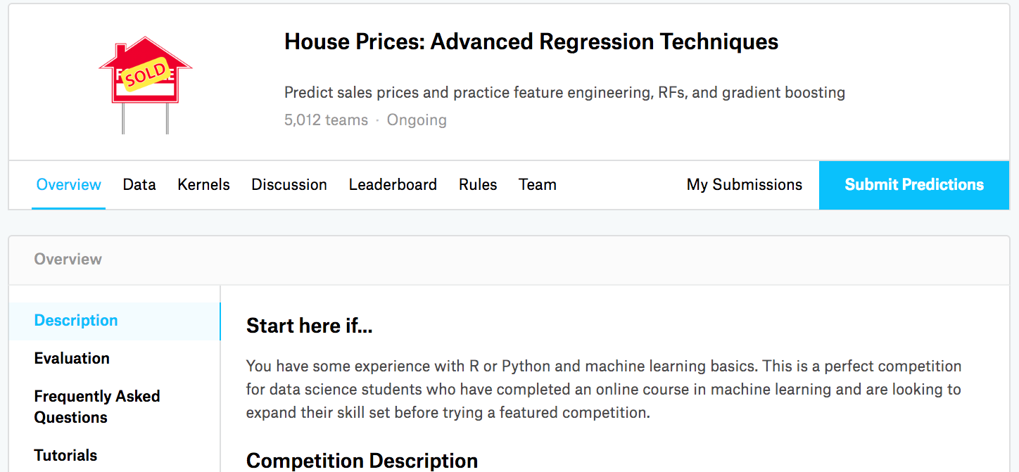
On the house price prediction competition page, as illustrated in Figure 4.7.2, you can find the dataset (under the “Data” tab), submit predictions, and see your ranking. The URL is right here:
https://www.kaggle.com/c/house-prices-advanced-regression-techniques
4.7.2 Accessing and Reading the Dataset
Note that the competition data is separated into training and test sets. Each record includes the property value of the house and attributes such as street type, year of construction, roof type, basement condition, etc. The features consist of various data types. For example, the year of construction is represented by an integer, the roof type by discrete categorical assignments, and other features by floating point numbers. Some examples have missing values, represented as “na”. The price of each house is included for the training set only (it is a competition after all). We will want to partition the training set to create a validation set, but we only get to evaluate our models on the official test set after uploading predictions to Kaggle. The “Data” tab on the competition tab in Figure 4.7.2 has links for downloading the data.
To get started, we will read in and process the data using pandas, which we introduced in Section 1.2. For convenience, we use the d2l.download helper to fetch and cache the Kaggle housing dataset. It performs hash-checked caching: if a file corresponding to this dataset already exists in the cache directory and its SHA-1 matches sha1_hash, the cached copy is reused, avoiding redundant downloads (its implementation details live in the d2l library).
class KaggleHouse(d2l.DataModule):
    def __init__(self, batch_size, train=None, val=None):
        super().__init__()
        self.save_hyperparameters()
        if self.train is None:
            self.raw_train = pd.read_csv(d2l.download(
                d2l.DATA_URL + 'kaggle_house_pred_train.csv', self.root,
                sha1_hash='585e9cc93e70b39160e7921475f9bcd7d31219ce'))
            self.raw_val = pd.read_csv(d2l.download(
                d2l.DATA_URL + 'kaggle_house_pred_test.csv', self.root,
                sha1_hash='fa19780a7b011d9b009e8bff8e99922a8ee2eb90'))
The training dataset includes 1460 examples, 80 features, and one label, while the Kaggle test set contains 1459 examples and 80 features. (We store the test features in the val attribute because the data module treats any unlabeled held-out split uniformly; do not confuse it with the validation folds that we will carve out of the training data for cross-validation below.)
data = KaggleHouse(batch_size=64)
print(data.raw_train.shape)
print(data.raw_val.shape)
(1460, 81)
(1459, 80)4.7.3 Data Preprocessing
We inspect the first four and final two features, together with the label (SalePrice), for the first four examples.
print(data.raw_train.iloc[:4, [0, 1, 2, 3, -3, -2, -1]]) Id MSSubClass MSZoning LotFrontage SaleType SaleCondition SalePrice
0 1 60 RL 65.0 WD Normal 208500
1 2 20 RL 80.0 WD Normal 181500
2 3 60 RL 68.0 WD Normal 223500
3 4 70 RL 60.0 WD Abnorml 140000We can see that in each example, the first feature is the identifier, which lets us identify each record. We drop it here because the competition defines it as a row identifier rather than a measured house attribute. Identifiers are not harmless in every dataset: they can encode collection order, source, or time, so one should check what they encode rather than drop them by rule. Furthermore, given a wide variety of data types, we will need to preprocess the data before we can start modeling.
We begin with the numerical features. First, we apply a heuristic, replacing all missing values by the corresponding feature’s mean. Then, to put all features on a common scale, we standardize the data by rescaling features to zero mean and unit variance:
\[x \leftarrow \frac{x - \mu}{\sigma}, \tag{4.7.1}\]
where \(\mu\) and \(\sigma\) denote the feature’s mean and standard deviation. By the definition of mean and variance, the rescaled feature has
\[ E\!\left[\frac{x-\mu}{\sigma}\right] = 0 \qquad \textrm{and} \qquad \mathrm{Var}\!\left[\frac{x-\mu}{\sigma}\right] = 1, \]
so every column now has zero mean and unit variance. We compute \(\mu\) and \(\sigma\) from the training set only and apply the very same transformation to the test set. Using statistics that include the test data would let information about the test distribution seep into our preprocessing, optimistically biasing every evaluation we make afterwards. This pitfall is called test-set leakage, and it is one of the most common ways a model looks better offline than it ever does in deployment.
Intuitively, we standardize the data for three reasons. First, it proves convenient for optimization, putting all coordinates on a comparable scale. Second, because we do not know a priori which features will be relevant, we do not want to penalize coefficients assigned to one feature more than any other (a single scale lets weight decay treat them even-handedly). Third, it makes our mean-imputation step coherent: after standardization, filling a missing value with the column mean is exactly filling it with \(0\), the same neutral value regardless of the feature’s original units.
Next we deal with discrete values. These include features such as “MSZoning”. We replace them by a one-hot encoding in the same way that we earlier transformed multiclass labels into vectors (see Section 3.1.1). For instance, “MSZoning” assumes the values “RL” and “RM”. Dropping the “MSZoning” feature, we create two new indicator features “MSZoning_RL” and “MSZoning_RM” whose values are either 0 or 1. According to one-hot encoding, if the original value of “MSZoning” is “RL”, then “MSZoning_RL” is 1 and “MSZoning_RM” is 0. The pandas package does this automatically for us. We also fit the categorical vocabulary on the training rows only. At validation or deployment time, a category unseen during fitting maps to all zeros for that feature’s known indicators. Building the vocabulary from an unlabeled test batch is a transductive competition technique; it is unsuitable when future categories are unavailable during training.
@d2l.add_to_class(KaggleHouse)
def preprocess(self):
    self.train, self.val = fit_preprocess(self.raw_train, self.raw_val)

def fit_preprocess(train_raw, other_raw):
    """Fit preprocessing on train_raw and apply it to both dataframes."""
    label = 'SalePrice'
    train_X = train_raw.drop(columns=['Id', label])
    other_X = other_raw.drop(columns=['Id', label], errors='ignore')
    numeric = train_X.select_dtypes(include='number').columns
    train_X[numeric] = train_X[numeric].astype(float)
    other_X[numeric] = other_X[numeric].astype(float)
    mean, std = train_X[numeric].mean(), train_X[numeric].std()
    std = std.mask(std == 0, 1)
    train_X.loc[:, numeric] = (train_X[numeric] - mean) / std
    other_X.loc[:, numeric] = (other_X[numeric] - mean) / std
    train_X.loc[:, numeric] = train_X[numeric].fillna(0)
    other_X.loc[:, numeric] = other_X[numeric].fillna(0)
    train_X = pd.get_dummies(train_X, dummy_na=True)
    other_X = pd.get_dummies(other_X, dummy_na=True)
    other_X = other_X.reindex(columns=train_X.columns, fill_value=0)
    train_X[label] = train_raw[label].values
    if label in other_raw:
        other_X[label] = other_raw[label].values
    return train_X, other_X
You can see that this conversion expands the 79 raw predictors into several hundred numeric columns; the exact count is determined by the categories observed in the training data.
data.preprocess()
data.train.shape
(1460, 331)4.7.4 Error Measure
Before choosing a model, we need to decide what “good” means: the loss we train against and the metric we are scored on. So the choice of error measure comes first.
With house prices, as with stock prices, we care about relative quantities more than absolute quantities. Thus we tend to care more about the relative error \(\frac{y - \hat{y}}{y}\) than about the absolute error \(y - \hat{y}\). For instance, if our prediction is off by $100,000 when estimating the price of a house in rural Ohio, where the value of a typical house is $125,000, then the relative error is large. If we err by the same amount in Los Altos Hills, California, the relative error may instead be small (there, the median house price exceeds $4 million).
One way to address this problem is to measure the discrepancy in the logarithm of the price estimates. In fact, this is also the official error measure used by the competition to evaluate the quality of submissions. After all, a small value \(\delta\) for \(|\log y - \log \hat{y}| \leq \delta\) translates into \(e^{-\delta} \leq \frac{\hat{y}}{y} \leq e^\delta\). This leads to the following root-mean-squared-error between the logarithm of the predicted price and the logarithm of the label price:
\[\sqrt{\frac{1}{n}\sum_{i=1}^n\left(\log y_i -\log \hat{y}_i\right)^2}. \tag{4.7.2}\]
@d2l.add_to_class(KaggleHouse)
def get_dataloader(self, train):
    label = 'SalePrice'
    data = self.train if train else self.val
    if label not in data: return
    get_tensor = lambda x: d2l.tensor(x.values.astype(float),
                                      dtype=d2l.float32)
    # Logarithm of prices
    tensors = (get_tensor(data.drop(columns=[label])),  # X
               d2l.reshape(d2l.log(get_tensor(data[label])), (-1, 1)))  # Y
    return self.get_tensorloader(tensors, train)
4.7.5 \(K\)-Fold Cross-Validation
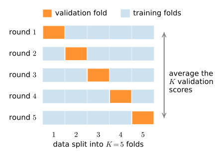
You might recall that we introduced cross-validation in Section 2.6.3, where we discussed how to deal with model selection. We will put this to good use to select the model design and to adjust the hyperparameters. The idea is shown in Figure 4.7.3: we partition the data into \(K\) folds whose sizes differ by at most one and run \(K\) training rounds. In round \(i\), fold \(i\) is held out for validation and the model is trained on the remaining \(K-1\) folds; our generalization estimate is the average of the \(K\) validation scores. With only about \(1500\) training examples here, this reuse of the data gives a far steadier estimate than any single train/validation split would.
We first need a function that returns the \(i^\textrm{th}\) fold of the data in a \(K\)-fold cross-validation procedure. It proceeds by slicing out the \(i^\textrm{th}\) segment as validation data and returning the rest as training data. Note that this is not the most efficient way of handling data and we would definitely do something much smarter if our dataset was considerably larger. But this added complexity might obfuscate our code unnecessarily so we can safely omit it here owing to the simplicity of our problem.
def k_fold_data(data, k):
    rets = []
    indices = data.raw_train.sample(frac=1, random_state=0).index.tolist()
    base, remainder = divmod(len(indices), k)
    start = 0
    for j in range(k):
        stop = start + base + (j < remainder)
        val_idx = indices[start:stop]
        raw_train = data.raw_train.drop(index=val_idx)
        raw_val = data.raw_train.loc[val_idx]
        train, val = fit_preprocess(raw_train, raw_val)
        _, test = fit_preprocess(raw_train, data.raw_val)
        fold = KaggleHouse(data.batch_size, train, val)
        fold.test = test
        rets.append(fold)
        start = stop
    return rets
We train \(K\) times in the \(K\)-fold cross-validation and return the average validation error. We pass in a model_fn that builds a fresh model for each fold, so the same cross-validation loop can score a linear baseline or an MLP without change.
def k_fold(trainer, data, k, model_fn):
    val_loss, models = [], []
    for i, data_fold in enumerate(k_fold_data(data, k)):
        model = model_fn()
        model.board.yscale='log'
        if i != 0: model.board.display = False
        trainer.fit(model, data_fold)
        val_loss.append(float(model.board.data['val_loss'][-1].y))
        models.append((model, data_fold.test))
    mean = sum(val_loss) / len(val_loss)
    sd = (sum((x - mean) ** 2 for x in val_loss) / (len(val_loss) - 1)) ** 0.5
    scores = ', '.join(f'{x:.4f}' for x in val_loss)
    print(f'fold validation log mse = [{scores}]')
    print(f'mean = {mean:.4f}; sd = {sd:.4f}')
    return models
def k_fold(trainer, data, k, model_fn):
val_loss, models = [], []
for i, data_fold in enumerate(k_fold_data(data, k)):
model = model_fn()
model.board.yscale='log'
if i != 0: model.board.display = False
trainer.fit(model, data_fold)
val_loss.append(float(model.board.data['val_loss'][-1].y))
models.append((model, data_fold.test))
mean = sum(val_loss) / len(val_loss)
sd = (sum((x - mean) ** 2 for x in val_loss) / (len(val_loss) - 1)) ** 0.5
scores = ', '.join(f'{x:.4f}' for x in val_loss)
print(f'fold validation log mse = [{scores}]')
print(f'mean = {mean:.4f}; sd = {sd:.4f}')
return modelsdef k_fold(trainer, data, k, model_fn):
val_loss, models = [], []
for i, data_fold in enumerate(k_fold_data(data, k)):
# One-hot vocabularies are fitted within each fold, so the number of
# input columns can differ slightly between folds.
model = model_fn(data_fold)
model.board.yscale='log'
if i != 0: model.board.display = False
trainer.fit(model, data_fold)
val_loss.append(float(model.board.data['val_loss'][-1].y))
models.append((model, data_fold.test))
mean = sum(val_loss) / len(val_loss)
sd = (sum((x - mean) ** 2 for x in val_loss) / (len(val_loss) - 1)) ** 0.5
scores = ', '.join(f'{x:.4f}' for x in val_loss)
print(f'fold validation log mse = [{scores}]')
print(f'mean = {mean:.4f}; sd = {sd:.4f}')
return modelsdef k_fold(trainer, data, k, model_fn):
val_loss, models = [], []
for i, data_fold in enumerate(k_fold_data(data, k)):
model = model_fn()
model.board.yscale='log'
if i != 0: model.board.display = False
trainer.fit(model, data_fold)
val_loss.append(float(model.board.data['val_loss'][-1].y))
models.append((model, data_fold.test))
mean = sum(val_loss) / len(val_loss)
sd = (sum((x - mean) ** 2 for x in val_loss) / (len(val_loss) - 1)) ** 0.5
scores = ', '.join(f'{x:.4f}' for x in val_loss)
print(f'fold validation log mse = [{scores}]')
print(f'mean = {mean:.4f}; sd = {sd:.4f}')
return models4.7.6 Model Selection
We now have everything we need to compare model designs by their \(K\)-fold cross-validation score. Finding a good choice can take time, depending on how many variables one optimizes over. With a large enough dataset, and the normal sorts of hyperparameters, \(K\)-fold cross-validation tends to be reasonably resilient against multiple testing. However, if we try an unreasonably large number of options we might find that our validation performance is no longer representative of the true error.
One caveat before we run the numbers. On structured tabular data like this dataset, gradient-boosted tree ensembles (XGBoost and LightGBM) typically outperform deep networks, including MLPs (Grinsztajn et al. 2022; Shwartz-Ziv and Armon 2022). This does not diminish what we learn here, since the preprocessing pipeline, log-RMSE loss, and \(K\)-fold cross-validation apply to any model class. But it does set expectations about where neural networks shine (images, text, audio, and sequences) and where they currently do not (small-to-medium tabular data).
We start with a linear model, a fast baseline that sanity-checks the pipeline. One subtlety is easy to get wrong: a baseline is only meaningful if it is trained competently. Plain minibatch SGD on these standardized features needs more than a handful of passes to converge, so we give the linear model a healthy \(100\) epochs at learning rate \(0.03\) (a larger rate diverges on the log-price target). Trained this way the linear model already reaches a cross-validated log error well under \(0.05\); stopping at the customary ten epochs would instead leave it badly underfit, which would flatter every model we compared against it.
trainer = d2l.Trainer(max_epochs=100)
linear_models = k_fold(trainer, data, k=5,
                       model_fn=lambda: d2l.LinearRegression(lr=0.03))
fold validation log mse = [0.0457, 0.0303, 0.0480, 0.0331, 0.0178]
mean = 0.0350; sd = 0.0123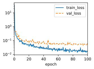
trainer = d2l.Trainer(max_epochs=100)
models = k_fold(trainer, data, k=5,
                model_fn=lambda: d2l.LinearRegression(lr=0.03))
fold validation log mse = [0.0702, 0.0336, 0.0392, 0.0355, 0.0197]
mean = 0.0396; sd = 0.0186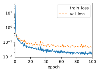
trainer = d2l.Trainer(max_epochs=100)
models = k_fold(
    trainer, data, k=5,
    model_fn=lambda fold: d2l.LinearRegression(
        fold.train.shape[1] - 1, lr=0.03))
fold validation log mse = [0.0478, 0.0282, 0.0400, 0.0345, 0.0191]
mean = 0.0339; sd = 0.0110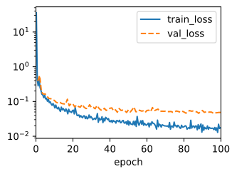
trainer = d2l.Trainer(max_epochs=100)
models = k_fold(trainer, data, k=5,
                model_fn=lambda: d2l.LinearRegression(lr=0.03))
fold validation log mse = [0.0418, 0.0279, 0.0411, 0.0326, 0.0359]
mean = 0.0359; sd = 0.0059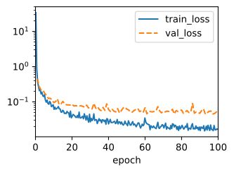
Can a small neural network do better? Now that we have weight decay (Section 2.7), dropout (Section 4.6), and sensible initialization (Section 4.4) in hand, we can try the simplest possible upgrade: a single hidden layer with a ReLU nonlinearity. The dataset is small (about \(1460\) rows and several hundred features after one-hot encoding), so we test a compact, regularized network: a \(32\)-unit hidden layer, a light dropout of \(0.1\), and a small amount of \(L_2\) weight decay (\(10^{-4}\)) added straight into SGD. These settings are one candidate rather than an established optimum; wider networks and different dropout rates require their own validation. We reuse the squared-error loss from LinearRegression and only override the optimizer to attach weight decay.
class KaggleMLP(d2l.LinearRegression):
    def __init__(self, lr, num_hiddens=32, dropout=0.1, weight_decay=1e-4):
        super(d2l.LinearRegression, self).__init__()
        self.save_hyperparameters()
        self.net = nn.Sequential(nn.LazyLinear(num_hiddens), nn.ReLU(),
                                 nn.Dropout(dropout), nn.LazyLinear(1))

    def configure_optimizers(self):
        return torch.optim.SGD(self.parameters(), lr=self.lr,
weight_decay=self.weight_decay)We train it with the same \(K\)-fold loop, learning rate, and epoch budget as the linear baseline. This controls the stated budget but does not guarantee that both model classes are equally well tuned.
trainer = d2l.Trainer(max_epochs=100)
models = k_fold(trainer, data, k=5, model_fn=lambda: KaggleMLP(lr=0.03))
fold validation log mse = [0.0506, 0.0276, 0.0538, 0.0188, 0.0289]
mean = 0.0359; sd = 0.0154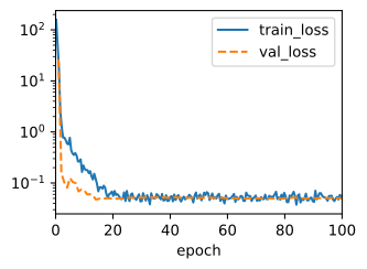
For the tested configurations, the small MLP has the lower mean cross-validated log error: about \(0.027\) versus \(0.036\) for the linear model. The fold-level dispersion printed above is necessary for judging this difference. This result applies only to the configurations and training budget tested here. Preprocessing and regularization make the MLP viable on a dataset of barely a thousand rows, and a longer training schedule improves both baselines. The preceding caveat motivates measuring a gradient-boosted tree ensemble rather than inferring its result. The exercises invite this comparison.
Notice that sometimes the number of training errors for a set of hyperparameters can be very low, even as the number of errors on \(K\)-fold cross-validation grows considerably higher. This indicates that we are overfitting. Throughout training you will want to monitor both numbers. Less overfitting might indicate that our data can support a more powerful model. Substantial overfitting may indicate that stronger regularization could help.
4.7.7 Submitting Predictions on Kaggle
After selecting hyperparameters by cross-validation, we average the predictions of the \(K\) models on the test set. Since the models predict log-prices and the competition scores root-mean-squared log error, we average in log space before exponentiating: the mean of the log-predictions is the ensemble consistent with the metric (in price space it amounts to a geometric mean).
This fold ensembling deserves a closer look, though. Each of the \(K\) models saw only \((K-1)/K\) of the training data, so the “average validation log mse” we computed above estimates the error of a single such model; it does not measure the error of the ensemble we are about to submit. An alternative is to refit one model on all of the training data using the hyperparameters selected by cross-validation. Fold ensembling reuses the \(K\) trained models, and averaging their predictions usually reduces variance. Refitting instead trains on every available example. These procedures estimate and use the data differently, so their performance should be compared empirically.
Saving the predictions in a csv file will simplify uploading the results to Kaggle. The following code will generate a file called submission.csv.
for model, _ in models:
    model.eval()  # already the case after Trainer.fit; explicit is safer
preds = [model(d2l.tensor(test.values.astype(float), dtype=d2l.float32))
         for model, test in models]
# Each model predicts a log-price; average across the K folds in log space,
# then exponentiate back to a price.
ensemble_preds = d2l.exp(d2l.reduce_mean(d2l.concat(preds, 1), 1))
submission = pd.DataFrame({'Id':data.raw_val.Id,
                           'SalePrice':d2l.numpy(ensemble_preds)})
submission.to_csv('submission.csv', index=False)
preds = [model(d2l.tensor(test.values.astype(float), dtype=d2l.float32))
for model, test in models]
# Average the K log-price predictions in log space, then exponentiate.
ensemble_preds = d2l.exp(d2l.reduce_mean(d2l.concat(preds, 1), 1))
submission = pd.DataFrame({'Id':data.raw_val.Id,
'SalePrice':d2l.numpy(ensemble_preds)})
submission.to_csv('submission.csv', index=False)preds = [model(d2l.tensor(test.values.astype(float), dtype=d2l.float32))
for model, test in models]
# Average the K log-price predictions in log space, then exponentiate.
ensemble_preds = d2l.exp(d2l.reduce_mean(d2l.concat(preds, 1), 1))
submission = pd.DataFrame({'Id':data.raw_val.Id,
'SalePrice':d2l.numpy(ensemble_preds)})
submission.to_csv('submission.csv', index=False)preds = [model(d2l.tensor(test.values.astype(float), dtype=d2l.float32))
for model, test in models]
# Average the K log-price predictions in log space, then exponentiate.
ensemble_preds = d2l.exp(d2l.reduce_mean(d2l.concat(preds, 1), 1))
submission = pd.DataFrame({'Id':data.raw_val.Id,
'SalePrice':d2l.numpy(ensemble_preds)})
submission.to_csv('submission.csv', index=False)Next, as demonstrated in Figure 4.7.4, we can submit our predictions on Kaggle and see how they compare with the actual house prices (labels) on the test set. The steps are quite simple:
- Log in to the Kaggle website and visit the house price prediction competition page.
- Click the “Submit Predictions” or “Late Submission” button.
- Click the “Upload Submission File” button in the dashed box at the bottom of the page and select the prediction file you wish to upload.
- Click the “Make Submission” button at the bottom of the page to view your results.

4.7.8 Summary and Discussion
Real data is messy: a mix of numeric and categorical features, with missing values and wildly different scales. The preprocessing pipeline in this section is a sensible default that applies far beyond this competition: mean imputation, standardization with statistics fit on the training set only to avoid test-set leakage, and one-hot encoding of categoricals. When the target spans an order of magnitude, predicting the logarithm of the price and scoring with root-mean-squared log error converts an asymmetric dollar-scale problem into one where a \(10\%\) error on a \(\$100{,}000\) house and on a \(\$1{,}000{,}000\) house are penalized equally, which is what we actually care about.
\(K\)-fold cross-validation is useful for limited IID data such as this dataset: it spends \(K\) training runs to reduce dependence on one validation split, and the same loop supports hyperparameter search. Random folds are invalid when rows are grouped, ordered in time, spatially dependent, or otherwise linked; those settings require a split that preserves the dependence structure.
Two caveats belong in any account of this pipeline. First, none of it is specific to neural networks: the same preprocessing, loss design, and cross-validation loop work with any model class, including the gradient-boosted tree ensembles (XGBoost, LightGBM) that routinely beat deep networks on medium-sized tabular data (Grinsztajn et al. 2022; Shwartz-Ziv and Armon 2022). Second, model capacity matters: adding hidden layers, tuning the dropout rate, and searching over learning rate and weight decay can improve substantially on the baseline shown here, which is exactly what the exercises ask you to do.
The methods used here recur throughout supervised learning. Feature scaling and imputation reappear in nearly every tabular pipeline, and the competition recipe (download, preprocess, match the loss to the metric, cross-validate, refit, submit) generalizes directly: later chapters apply the same cross-validation discipline to image datasets, sequence tasks, and the fine-tuning of pretrained models.
4.7.9 Exercises
[code] Fold ensembling versus refitting. Section 4.7.7 describes two ways of producing a final model after cross-validation: averaging the \(K\) fold models’ predictions, or refitting one model on the complete training set with the selected hyperparameters.
- Submit the
submission.csvthat this section writes, which holds the fold ensemble’s predictions, to Kaggle. The leaderboard reports the root-mean-squared log error, whereask_foldprints the mean squared error of the log prices. Convert the mean thatk_foldprints to the leaderboard’s scale and compare it with your score. - Refit one model on the complete training set with the same hyperparameters, submit its predictions, and compare the two leaderboard scores.
- Explain why the training error of the refit model is not a substitute for the cross-validated estimate.
- Submit the
[code] Mean imputation.
fit_preprocessreplaces every missing numerical value by the training-set mean of its column. Its call topd.get_dummieswithdummy_na=Truealso adds a missing-value indicator column for every categorical feature.- Identify a numerical feature in this dataset whose missingness is not random with respect to the sale price.
- Explain what bias mean imputation alone would introduce for that feature, and in which direction it would shift the predictions for the affected houses. Then determine whether the indicator columns that
fit_preprocessalready creates let a linear model remove this bias. - Replace mean imputation by median imputation, and separately add a binary missingness indicator column for each imputed feature. Compare the cross-validated errors of the three variants.
Adapted from Kaggle Learn, Intermediate Machine Learning, Exercise 2.
[code] Improving the score. ● Start from the linear model
d2l.LinearRegressionwith learning rate \(0.03\) that this section cross-validates. Lower its cross-validated error, and then the leaderboard score.- Holding the model fixed, tune the learning rate, the number of epochs, and the strength of an \(L_2\) weight-decay penalty, added as in Section 2.7, by \(K\)-fold cross-validation.
- Replace the linear model by an MLP, and vary the number and width of its hidden layers and its dropout rate. Which change helps most, and does the gain survive on the leaderboard?
[code] Skipping standardization. Remove the standardization from
fit_preprocess. Becausefillna(0)imputes the column mean only for standardized columns, fill missing numerical values with the training-set column means explicitly instead.- Rerun the \(K\)-fold cross-validation of the linear model at the section’s learning rate of \(0.03\), and describe the training loss.
- Find, to within a factor of ten, the largest learning rate at which the unstandardized linear model trains without diverging. Compare its cross-validated error after \(100\) epochs with that of the standardized pipeline, and explain both observations.
[code] Gradient-boosted trees. Fit a gradient-boosted tree model (for example scikit-learn’s
GradientBoostingRegressor, or XGBoost or LightGBM if installed) to the log sale price, using the preprocessed training rows of each fold thatk_fold_data(data, 5)returns. Score it on each validation fold by the mean squared error of the log price, the quantity thatk_foldprints, and compare the mean over folds with that of the models trained in this section. Why might tree ensembles have an edge on data like this?[code] Encoding categorical features.
fit_preprocessone-hot encodes every categorical column by callingpd.get_dummieswithdummy_na=True. Find the categorical column with the most distinct values in the training data, and determine how many columns of the feature matrix its one-hot encoding occupies.Adapted from Kaggle Learn, Intermediate Machine Learning, Exercise 3.
[code] Target encoding. ● Target encoding replaces each category of a categorical column by the mean log sale price of the training rows in that category, so that the feature occupies a single column instead of the one column per category that
fit_preprocesscreates.- Target-encode every categorical column with more than ten categories instead of one-hot encoding it, computing the category means from the training rows of each fold. Give a category that does not occur in those rows the overall mean, and standardize the encoded columns like the numerical features. Compare the cross-validated error with that of one-hot encoding.
- The encoding above computes each training row’s value from a mean that includes that row’s own label. Encode the training rows out of fold instead: split the training rows of each fold into five parts, and encode each part with category means computed from the other four parts. Compare the cross-validated error with that of the in-sample encoding, and explain how the size of a category affects the difference between the two encodings.
[code] Target leakage. A feature that is recorded only after, or because of, the event being predicted inflates validation scores without helping a deployed model.
- Identify at least one raw feature in this dataset that could plausibly be filled in only after the sale, and explain why cross-validation does not catch the problem.
- Verify the mechanism empirically: add a synthetic feature equal to the log sale price plus small Gaussian noise, rerun the \(K\)-fold cross-validation, and report the change in the error that
k_foldprints.
Adapted from Kaggle Learn, Intermediate Machine Learning, Exercise 7.
Geometric averaging. ● Section 4.7.7 averages the \(K\) fold models’ log-price predictions \(z_1, \ldots, z_K\) for a house before exponentiating, which amounts to a geometric mean in price space.
Compare \(\exp\bigl(\frac{1}{K}\sum_{k=1}^K z_k\bigr)\) with the price-space average \(\frac{1}{K}\sum_{k=1}^K e^{z_k}\). Show which of the two never exceeds the other, and state when they coincide.
Let \(\log y\) be the true log price of the house. Show that the log-space average satisfies
\[\Bigl(\log y - \frac{1}{K}\sum_{k=1}^K z_k\Bigr)^2 \leq \frac{1}{K}\sum_{k=1}^K \left(\log y - z_k\right)^2. \tag{4.7.3}\]
Determine whether the logarithm of the price-space average satisfies the same bound for all predictions \(z_1, \ldots, z_K\).