import math
import torch28.1 Entropy, Cross-Entropy, and KL Divergence
Cross-entropy is one of the most common training losses in this book. It is also a basic quantity in information theory, introduced by Shannon in 1948 (Shannon 1948). Its coding interpretation relates three quantities: entropy is the expected code length under the data distribution, cross-entropy is the expected length obtained with a model distribution, and their difference is the Kullback–Leibler divergence. This section develops these quantities and Gibbs’ inequality, derives their coding interpretation from the Kraft inequality and Shannon codes, and explains perplexity, label smoothing, and knowledge distillation in the same framework.
The logarithm base is a pure choice of unit: base \(2\) gives bits, base \(e\) gives nats. We work in nats throughout, matching deep-learning practice: the library log is natural, so reported training losses are already in nats. The one place where base \(2\) is genuinely natural is coding with binary symbols, and we flag it explicitly when we get there. Since \(\log_2 x = \ln x / \ln 2\), converting is a fixed rescaling: \(1\textrm{ bit} = \ln 2 \approx 0.693\) nats and \(1\textrm{ nat} = 1/\ln 2 \approx 1.443\) bits. Changing the logarithm base leaves every argmin and trained model unchanged.
We use the following imports throughout the section.
import math
import tensorflow as tf
import math
import jax
from jax import numpy as jnp
import optaximport math
from mxnet import autograd, np, npx
npx.set_np()28.1.1 Information and Entropy
28.1.1.1 Surprise and Self-Information
Consider reports about a shuffled deck of cards. “I see a card” conveys no new information because the event is certain. “I see a heart” identifies one of four equally likely suits, while “It is the three of spades” identifies one of \(52\) equally likely cards. The order of the entire deck identifies one of \(52!\) outcomes. Information therefore tracks surprise: the less probable an event, the more is learned by observing it. Shannon formalized this idea. The self-information of an event \(x\) with probability \(p(x)\) is
\[ I(x) = -\log p(x), \]
measured in nats for the natural logarithm. The four card reports carry \(-\ln 1 = 0\), \(\ln 4 \approx 1.39\), \(\ln 52 \approx 3.95\), and \(\ln 52! \approx 156.4\) nats respectively; in bits (base \(2\), the unit of one fair coin flip) they carry the classic numbers \(0\), \(2\), \(\log_2 52 \approx 5.70\), and \(\log_2 52! \approx 225.6\). The function \(-\log p\) is the unique choice (up to the base, i.e., the unit) satisfying the properties we implicitly demanded: certain events carry zero information, rarer events carry more, and independent events add, so that \(I\) of a joint outcome with probability \(p_1 p_2\) is \(I(p_1) + I(p_2)\), which forces a logarithm (Csiszár (2008) gives the formal axiomatics; Exercise 5 walks through the argument).
This surprise is relative to the stated probabilistic model and its event partition. A confidently incorrect model can assign large self-information to an ordinary event; the number alone does not measure semantic importance or anomaly.
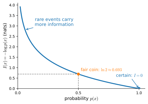
Figure 28.1.1 plots the curve: decreasing, convex, zero at \(p = 1\), infinite at \(p = 0\). The computation is immediate.
import numpy as onp
def self_information(p):
    """Self-information -log p, in nats."""
    return -onp.log(p)

self_information(1 / 64)np.float64(4.1588830833596715)np.float64(4.1588830833596715)np.float64(4.1588830833596715)4.1588830833596715An event of probability \(1/64\) carries \(\ln 64 \approx 4.16\) nats (exactly \(6\) bits: it takes six fair-coin flips to have probability \(1/64\)).
28.1.1.2 Shannon Entropy
Let \(X\) be a discrete random variable with probability mass function \(p\). Its Shannon entropy is the expected self-information of its outcome:
\[H(X) = - E_{x \sim P} [\log p(x)]. \tag{28.1.1}\]
Equivalently, \(H(X)=-\sum_i p_i\log p_i\), where \(p_i=P(X=x_i)\). A point mass has entropy zero, and a distribution on a fixed finite support has maximal entropy when it is uniform. These nonnegativity and coding interpretations apply to probability masses. They must not be transferred to density values, which can exceed one and change under a coordinate transformation.
For continuous \(X\) with density \(p\) the sum becomes an integral, and the result is called the differential entropy,
\[ h(X) = -\int p(x) \log p(x) \,dx. \tag{28.1.2}\]
We write lowercase \(h\) for differential entropy throughout, to keep it distinct from the discrete \(H\); the two behave differently in ways that matter. Differential entropy is not the limit of the discrete entropy, and it is not coordinate-invariant: under an invertible change of variables \(y = g(x)\) it shifts by \(E[\log|\det \partial g/\partial x|]\), so \(h\) can even be negative (e.g., a narrow Gaussian with \(\sigma < 1/\sqrt{2\pi e}\)). Quantities built from the ratio of two densities are invariant under a change of variables: both densities pick up the same Jacobian factor, which cancels in \(p(x)/q(x)\), so the KL divergence defined below is exactly invariant. Cross-entropy sits in between. It contains a single lone logarithm, \(-E_P[\log q]\), so it inherits the same Jacobian shift as entropy, but that shift depends only on the truth \(P\) and the map \(g\), never on the model \(Q\), so it moves every candidate model’s loss by the same constant. Reparameterizing the data changes all the cross-entropy values, but their differences, their gradients in \(Q\), and the argmin do not. That is the precise sense in which objectives that compare distributions are safe under reparameterization while raw differential entropy is not.
The convention \(0\log0=0\) should be implemented by masking only zero probabilities. A general nansum would also hide NaNs caused by negative, unnormalized, or otherwise invalid input, so the helper validates the vector.
import numpy as onp
def entropy(p):
    """Entropy of a probability vector, in nats."""
    p = onp.asarray(p, dtype=float)
    if p.ndim != 1 or not onp.all(onp.isfinite(p)):
        raise ValueError("p must be a finite one-dimensional probability vector")
    if onp.any(p < 0):
        raise ValueError("probabilities must be nonnegative")
    if not onp.isclose(p.sum(), 1.0):
        raise ValueError("probabilities must sum to one")
    positive = p > 0
    return float(-onp.dot(p[positive], onp.log(p[positive])))

entropy(onp.array([0.1, 0.5, 0.1, 0.3]))1.1682824501765625The distribution \((0.1, 0.5, 0.1, 0.3)\) has entropy \(\approx 1.168\) nats: less than the \(\ln 4 \approx 1.386\) nats of a uniform distribution on four outcomes, because the mass is unevenly spread.
28.1.1.3 Entropy Is Maximized by the Uniform Distribution
Two basic properties characterize discrete entropy. First, for discrete \(X\) every term \(-p_i \log p_i\) is non-negative, so \(H(X) \geq 0\), with equality exactly for a point mass (a constant “random” variable). Second, entropy is largest when the distribution hedges maximally:
Proposition (uniform maximizes entropy). If \(X\) takes at most \(k\) values, then
\[ H(X) \leq \log k, \]
with equality if and only if \(X\) is uniform on \(k\) values.
Proof. Write the entropy as an expectation of a concave function’s argument: \(H(X) = E[\log(1/p(X))]\). Since \(\log\) is concave, Jensen’s inequality (Section 26.3.3) gives
\[ H(X) = E\!\left[\log \frac{1}{p(X)}\right] \leq \log E\!\left[\frac{1}{p(X)}\right] = \log \sum_{i\,:\,p_i > 0} p_i \cdot \frac{1}{p_i} = \log m \leq \log k, \]
where \(m \leq k\) is the number of outcomes with \(p_i > 0\). Equality requires both inequalities to be tight. Because \(\log\) is strictly concave, the first is an equality only when \(1/p(X)\) is constant almost surely, i.e., \(X\) is uniform on its \(m\) support points; and \(\log m = \log k\) forces \(m = k\). Together: \(p_i = 1/k\) for all \(i\). \(\blacksquare\)
For continuous \(X\) the analogous statements need constraints to be true at all (on a bounded interval the uniform density again maximizes differential entropy; under a variance constraint the Gaussian does, as we prove in Section 28.1.2.3).
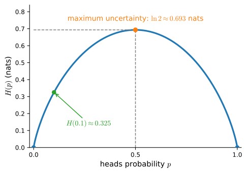
Consider the coin. A Bernoulli variable with heads-probability \(p\) has the binary entropy \(H(p) = -p \log p - (1-p)\log(1-p)\) (overloading \(H\): the argument here is a parameter, not a random variable), plotted in Figure 28.1.2: zero at the deterministic endpoints \(p \in \{0, 1\}\), concave in between, and maximal at the fair coin \(p = \tfrac{1}{2}\), where it equals \(\ln 2 \approx 0.693\) nats (\(= 1\) bit, consistent with the \(\log k\) bound for \(k = 2\)). A biased coin with \(p = 0.1\) has entropy \(H(0.1) \approx 0.325\) nats because its outcome is comparatively predictable.
Entropy also extends from one random variable to several: the joint entropy \(H(X, Y)\), the conditional entropy \(H(Y \mid X)\), and the mutual information \(I(X; Y)\) that measures what \(X\) and \(Y\) share. Those quantities power contrastive and self-supervised learning, and we develop them in their own section, Section 28.3.
28.1.2 Cross-Entropy and KL Divergence
28.1.2.1 The Kullback–Leibler Divergence
In Section 1.3 we measured distances between points with norms. We now want a notion of “distance” between distributions: how badly does a model \(Q\) misrepresent a truth \(P\)? Information theory’s answer is the Kullback–Leibler (KL) divergence, also called relative entropy (Kullback and Leibler 1951). Given a random variable \(X \sim P\) with p.d.f. or p.m.f. \(p(x)\), and a second distribution \(Q\) with p.d.f. or p.m.f. \(q(x)\) that we use to approximate \(P\),
\[D_{\textrm{KL}}(P\|Q) = E_{x \sim P} \left[ \log \frac{p(x)}{q(x)} \right]. \tag{28.1.3}\]
The term inside the expectation is \(\log p(x) - \log q(x)\), the difference of two surprises: how surprised \(Q\) is by the outcome \(x\), minus how surprised \(P\) is. It is positive where \(Q\) underestimates (\(q(x) < p(x)\): \(Q\) is more surprised than it should be) and negative where \(Q\) overestimates. KL averages this relative surprise over outcomes drawn from the truth \(P\). Note the asymmetry baked into the definition: \(P\) supplies both the samples and the numerator. In general \(D_{\textrm{KL}}(P\|Q) \neq D_{\textrm{KL}}(Q\|P)\), and the gap can be large (we exhibit it numerically below); the consequences of which direction is optimized are taken up in Section 28.2. One more edge case to keep in mind: if some outcome has \(p(x) > 0\) but \(q(x) = 0\) (the model declares impossible an event with positive probability), then \(D_{\textrm{KL}}(P\|Q) = \infty\).
Here is the discrete case in code, for p and q given as probability vectors over the same finite outcome set. KL divergence is non-negative on its own (Gibbs’ inequality, next), so we do not wrap the result in abs(); doing so would teach the false idea that KL needs an absolute value to stay non-negative. The nansum is deliberate: where \(p(x) = 0\) the direct floating-point expression for \(0 \cdot \log(0/q)\) yields nan, which nansum drops to encode \(0 \log 0 = 0\); the other edge case, \(p(x) > 0\) with \(q(x) = 0\), instead yields \(+\infty\) (not nan), which nansum keeps, so the code correctly returns \(+\infty\) for that divergence.
import numpy as onp
def kl_divergence(p, q):
    """KL(P || Q) for two probability vectors, in nats."""
    p, q = onp.asarray(p, dtype=float), onp.asarray(q, dtype=float)
    kl = p * onp.log(p / q)
    return float(onp.nansum(kl))
28.1.2.2 Gibbs’ Inequality
The KL divergence cannot be negative, an observation going back to Gibbs (Gibbs 1902). Together with the cross-entropy decomposition below, this result justifies cross-entropy as a loss and supports the later coding and label-smoothing results.
Proposition (Gibbs’ inequality). For any distributions \(P\) and \(Q\) on the same space,
\[ D_{\textrm{KL}}(P\|Q) \geq 0, \]
with equality if and only if \(P = Q\).
Proof. One application of Jensen’s inequality (Section 26.3.3) to the convex function \(-\log\):
\[ \begin{aligned} D_{\textrm{KL}}(P\|Q) &= E_{x\sim P}\!\left[-\log\frac{q(x)}{p(x)}\right] \geq -\log E_{x\sim P}\!\left[\frac{q(x)}{p(x)}\right] \\ &= -\log \!\!\sum_{x\,:\,p(x)>0}\!\! q(x) = -\log Q(\textrm{supp}\,P) \geq 0. \end{aligned} \]
The expectation runs only over the support of \(P\), where the \(p(x)\) factors cancel, and what remains is the \(Q\)-mass of that support: a number \(Q(\textrm{supp}\,P) \leq 1\), whose negative log is therefore \(\geq 0\) (the same computation runs with integrals for densities, with the same convention at \(q = 0\)). For equality throughout, both inequalities must be tight: because \(-\log\) is strictly convex, the first is an equality only when the ratio \(q(x)/p(x)\) is constant \(P\)-almost surely, and the second requires \(Q(\textrm{supp}\,P) = 1\), i.e., \(Q\) puts no mass outside \(P\)’s support. Summing \(q(x) = c\,p(x)\) over the support then gives \(c = 1\), i.e., \(P = Q\). \(\blacksquare\)
28.1.2.3 Maximum Entropy and the Gaussian
Gibbs’ inequality has an immediate consequence for continuous distributions: among all densities with a given mean and variance, the Gaussian is the hardest to predict. Section 27.2 granted this fact; here is the proof.
Proposition (Gaussian maximum entropy). Among all densities \(p\) on \(\mathbb{R}\) with mean \(\mu\) and variance \(\sigma^2\),
\[ h(P) \leq \tfrac{1}{2}\log(2\pi e \sigma^2) = h(\mathcal{N}(\mu, \sigma^2)), \tag{28.1.4}\]
with equality if and only if \(P = \mathcal{N}(\mu, \sigma^2)\).
Proof. Let \(\varphi(x) = (2\pi\sigma^2)^{-1/2} e^{-(x-\mu)^2/(2\sigma^2)}\) be the Gaussian density. The key observation is that \(-\log \varphi(x) = \tfrac{1}{2}\log(2\pi\sigma^2) + \tfrac{(x-\mu)^2}{2\sigma^2}\) is a quadratic in \(x\), so its expectation under any density \(p\) with mean \(\mu\) and variance \(\sigma^2\) depends on \(p\) only through those two moments:
\[ -E_P[\log \varphi(x)] = \tfrac{1}{2}\log(2\pi\sigma^2) + \frac{E_P\big[(x-\mu)^2\big]}{2\sigma^2} = \tfrac{1}{2}\log(2\pi\sigma^2) + \tfrac{1}{2} = \tfrac{1}{2}\log(2\pi e \sigma^2). \]
Taking \(P = \mathcal{N}(\mu, \sigma^2)\) itself, this computes the Gaussian’s own differential entropy en route: \(h(\mathcal{N}(\mu, \sigma^2)) = \tfrac{1}{2}\log(2\pi e \sigma^2)\), the closed form quoted whenever a Gaussian entropy is needed (for instance in Section 28.3). Now apply Gibbs’ inequality, which holds for densities as noted above, with \(Q = \mathcal{N}(\mu, \sigma^2)\). Because \(E_P[\log \varphi]\) is finite, the divergence splits:
\[ 0 \leq D_{\textrm{KL}}\big(P \,\|\, \mathcal{N}(\mu, \sigma^2)\big) = E_P[\log p(x)] - E_P[\log \varphi(x)] = -h(P) + \tfrac{1}{2}\log(2\pi e \sigma^2). \]
Rearranging gives Equation 28.1.4. Equality holds exactly when the divergence vanishes, which by Gibbs’ equality case means \(P = \mathcal{N}(\mu, \sigma^2)\). \(\blacksquare\)
The bound works because the Gaussian’s log-density is a polynomial in exactly the quantities being constrained, the first two moments, so the cross term \(-E_P[\log \varphi]\) is the same for every competitor \(P\).
28.1.2.4 Gaussians, in Closed Form
The kl_divergence above works on discrete probability vectors. For continuous distributions the standard worked example is the KL divergence between two univariate Gaussians, which has a closed form. For \(P = \mathcal{N}(\mu_1, \sigma_1^2)\) and \(Q = \mathcal{N}(\mu_2, \sigma_2^2)\),
\[ D_{\textrm{KL}}\!\left(\mathcal{N}(\mu_1,\sigma_1^2) \,\big\|\, \mathcal{N}(\mu_2,\sigma_2^2)\right) = \log\frac{\sigma_2}{\sigma_1} + \frac{\sigma_1^2 + (\mu_1 - \mu_2)^2}{2\sigma_2^2} - \frac{1}{2}. \tag{28.1.5}\]
These logs are natural logs, so the result is in nats. Read two things off Equation 28.1.5 directly. First, it is non-negative and zero exactly when \(\mu_1=\mu_2\) and \(\sigma_1=\sigma_2\) (i.e., \(P=Q\)), as Gibbs’ inequality demands. Second, it is not symmetric: swapping the roles of \(P\) and \(Q\) changes the value, because the variance ratio and the mean gap enter asymmetrically. (Deriving Equation 28.1.5 is Exercise 4.)
The following calculation compares the formula with a direct Monte Carlo estimate of \(D_{\textrm{KL}}(P\|Q) = E_{x\sim P}[\log p(x) - \log q(x)]\). The estimate uses no abs(); the divergence is non-negative on its own.
import numpy as onp
def gaussian_kl(mu1, sigma1, mu2, sigma2):
    """Closed-form KL(N(mu1, sigma1^2) || N(mu2, sigma2^2)), in nats."""
    return (math.log(sigma2 / sigma1)
            + (sigma1 ** 2 + (mu1 - mu2) ** 2) / (2 * sigma2 ** 2)
            - 0.5)

def gaussian_log_pdf(x, mu, sigma):
    return (-0.5 * math.log(2 * math.pi * sigma ** 2)
            - (x - mu) ** 2 / (2 * sigma ** 2))

def mc_kl(mu1, sigma1, mu2, sigma2, n=200000):
    """Monte-Carlo estimate of the same KL by sampling x ~ P."""
    x = onp.random.normal(loc=mu1, scale=sigma1, size=(n, ))
    return (gaussian_log_pdf(x, mu1, sigma1)
            - gaussian_log_pdf(x, mu2, sigma2)).mean()
Take \(P = \mathcal{N}(0, 1)\) and \(Q = \mathcal{N}(1, 1)\) (a unit mean shift, equal variances). The closed form should match the Monte-Carlo estimate to within sampling noise, and both should equal \(\tfrac{(\mu_1-\mu_2)^2}{2\sigma^2} = \tfrac{1}{2}\) nats here.
closed_form = gaussian_kl(0.0, 1.0, 1.0, 1.0)
monte_carlo = mc_kl(0.0, 1.0, 1.0, 1.0)

closed_form, monte_carlo(0.5, np.float64(0.5014436845909158))(0.5, np.float64(0.5002712449975965))(0.5, np.float64(0.4996905134959491))(0.5, 0.4958228465454059)Now make the asymmetry explicit. Compare \(D_{\textrm{KL}}(P\|Q)\) with \(D_{\textrm{KL}}(Q\|P)\) when the two Gaussians have different variances, say \(P=\mathcal{N}(0,1)\) and \(Q=\mathcal{N}(0,4)\) (i.e., \(\sigma_2=2\)). The two numbers differ (\(\approx 0.318\) vs. \(\approx 0.807\) nats): KL is a divergence, not a distance.
kl_pq = gaussian_kl(0.0, 1.0, 0.0, 2.0)
kl_qp = gaussian_kl(0.0, 2.0, 0.0, 1.0)

kl_pq, kl_qp
(0.3181471805599453, 0.8068528194400546)28.1.2.5 Cross-Entropy
The loss commonly implemented in classifiers is not the KL divergence but a close relative. The cross-entropy from \(P\) to \(Q\) scores outcomes drawn from the truth \(P\) by the model’s surprise,
\[\textrm{CE}(P, Q) = - E_{x \sim P} [\log q(x)]. \tag{28.1.6}\]
Adding and subtracting \(H(P)\) inside the expectation (legitimate whenever \(H(P)\) is finite) splits the model’s surprise into the truth’s own surprise plus the relative surprise:
\[\textrm{CE} (P, Q) = H(P) + D_{\textrm{KL}}(P\|Q). \tag{28.1.7}\]
Combined with Gibbs’ inequality, this identity explains why minimizing cross-entropy recovers the data distribution when the model family contains it:
\[ \underbrace{D_{\textrm{KL}}(P\|Q) \ge 0}_{\textrm{Gibbs}} \;\Longrightarrow\; \underbrace{\textrm{CE}(P,Q) \ge H(P)}_{\textrm{cross-entropy} \ \ge\ \textrm{entropy}}, \quad \textrm{equality iff } P = Q. \]
Entropy \(H(P)\) does not depend on the model \(Q\). Consequently, minimizing cross-entropy in \(Q\) is equivalent to minimizing \(D_{\textrm{KL}}(P\|Q)\), with equality at \(Q=P\). In the coding view below, these terms become expected code lengths. Figure 28.1.3 draws the decomposition to scale for a four-outcome distribution we will code by hand in that coding view.
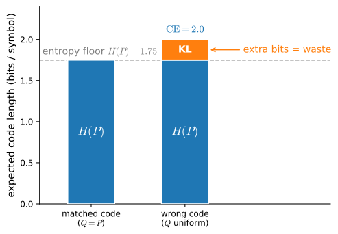
The following example verifies Equation 28.1.7 numerically on two small categorical distributions, and check the asymmetry of KL while we are at it.
import numpy as onp
p = onp.array([0.6, 0.3, 0.1])
q = onp.array([0.2, 0.5, 0.3])

ce_pq = float(-onp.sum(p * onp.log(q)))
print(f'KL(P||Q) = {kl_divergence(p, q):.4f} nats, '
      f'KL(Q||P) = {kl_divergence(q, p):.4f} nats')
print(f'CE(P, Q) - H(P) = {ce_pq - float(entropy(p)):.4f} nats')
KL(P||Q) = 0.3961 nats, KL(Q||P) = 0.3653 nats
CE(P, Q) - H(P) = 0.3961 natsThe forward and reverse KL disagree (\(\approx 0.396\) vs. \(\approx 0.365\) nats), and \(\textrm{CE} - H\) reproduces the forward KL exactly, as Equation 28.1.7 says it must.
28.1.2.6 The Classification Loss
In a \(k\)-class classification problem, the “truth” for one example is the one-hot distribution that puts all its mass on the correct label \(y\), and the model supplies a predicted distribution \(\hat{\mathbf{y}} = (\hat{y}_1, \ldots, \hat{y}_k)\). Cross-entropy Equation 28.1.6 between them collapses to a single term, \(-\log \hat{y}_{y}\): the model’s surprise at the correct class. Averaged over \(n\) examples, the cross-entropy loss is
\[ \textrm{CE}(\mathbf{y}, \hat{\mathbf{y}}) = -\frac{1}{n} \sum_{i=1}^n \log \hat{y}_{i, y_i}, \]
in nats, the mathematical quantity a built-in classification loss computes.
This display is the definition. Training code should supply logits to a from-logits loss, which performs the log-softmax without first rounding small probabilities to zero; Section 26.5.2 derives that implementation.
import numpy as onp
def cross_entropy(y_hat, y):
    """Mean cross-entropy loss for predicted probabilities, in nats."""
    ce = -onp.log(y_hat[range(len(y_hat)), y])
    return float(ce.mean())
Two examples, three classes: the first example’s true class is \(0\), predicted with probability \(0.3\); the second’s is \(2\), predicted with probability \(0.5\). The loss is \(\tfrac{1}{2}(-\ln 0.3 - \ln 0.5) \approx 0.949\) nats.
import numpy as onp
labels = onp.array([0, 2])
preds = onp.array([[0.3, 0.6, 0.1], [0.2, 0.3, 0.5]])

cross_entropy(preds, labels)0.9485599924429406The built-in loss computes the same number from logits \(\mathbf{z}\), applying log-softmax internally. We construct \(\mathbf{z}=\log\mathbf{q}\) only because the small example above starts from normalized probabilities; in a model, \(\mathbf{z}\) is the raw output of the final layer. Softmax inverts the log for a normalized \(\mathbf{q}\): \(\mathrm{softmax}(\log \mathbf{q})_j = e^{\log q_j} / \sum_i e^{\log q_i}
= q_j / \sum_i q_i = q_j\). (More generally, softmax is invariant to adding a constant to all logits, and \(\log\) of a normalized vector is one valid logit vector among many.) Passing probabilities to a loss intended for logits applies softmax twice; applying log to a computed softmax can underflow.
preds_torch = torch.tensor(preds, dtype=torch.float32)
labels_torch = torch.tensor(labels)
logits = torch.log(preds_torch)
torch.nn.CrossEntropyLoss()(logits, labels_torch)tensor(0.9486)preds_tf = tf.convert_to_tensor(preds, dtype=tf.float32)
labels_tf = tf.convert_to_tensor(labels)
logits = tf.math.log(preds_tf)
loss_fn = tf.keras.losses.SparseCategoricalCrossentropy(from_logits=True)
loss_fn(labels_tf, logits).numpy()np.float32(0.94856)preds_jax = jnp.asarray(preds)
labels_jax = jnp.asarray(labels)
logits = jnp.log(preds_jax)
optax.softmax_cross_entropy_with_integer_labels(
logits, labels_jax).mean()Array(0.94856, dtype=float32)preds_mx = np.array(preds.tolist())
labels_mx = np.array(labels.tolist())
logits = np.log(preds_mx)
log_probs = npx.log_softmax(logits, axis=1)
-log_probs[np.arange(len(labels_mx)), labels_mx].mean()array(0.9485576)The loss also has a decision-theoretic pedigree. A scoring rule assigns a penalty \(S(\mathbf{q}, y)\) for having reported the probability vector \(\mathbf{q}\) when class \(y\) then occurs. The rule is proper if truthful reporting is optimal: when the data-generating distribution is \(\mathbf{p}\), the expected penalty \(E_{y \sim \mathbf{p}}[S(\mathbf{q}, y)]\) is minimized by reporting \(\mathbf{q} = \mathbf{p}\), and strictly proper if this report is the unique optimum. The cross-entropy loss is the log score \(S(\mathbf{q}, y) = -\log q_y\), and it is strictly proper: its expected penalty is exactly \(\textrm{CE}(\mathbf{p}, \mathbf{q}) = H(\mathbf{p}) + D_{\textrm{KL}}(\mathbf{p} \| \mathbf{q})\), which Gibbs’ inequality minimizes uniquely at \(\mathbf{q} = \mathbf{p}\). Strict propriety of the log score is Gibbs’ inequality restated; Exercise 6 develops the argument.
Why insist on strict propriety? At population risk, over a model class that can represent the true conditional distribution, the log score is minimized by \(p(y \mid \mathbf{x})\) itself. That is the basis for calibration (predicted probabilities matching observed frequencies). Finite data, a restricted model class, regularization, imperfect optimization, and distribution shift can still produce miscalibration. Nor is the log score the only strictly proper rule: the Brier score \(S(\mathbf{q}, y) = \sum_j (q_j - \mathbf{1}[j = y])^2\) penalizes the whole vector by squared error, and its expected penalty exceeds the truthful reporter’s by \(\|\mathbf{q} - \mathbf{p}\|^2\): a squared-distance waste term in place of the KL-flavored one. Different strictly proper rules disagree about how severely to punish which mistakes (the log score’s penalty diverges on confident errors; the Brier score’s stays bounded), but they agree about where the optimum is: the truth (Gneiting and Raftery 2007).
For discrete observations, the average negative log-likelihood is exactly the cross-entropy from the empirical mass function to the model; its empirical entropy is constant in the model, so minimizing NLL also minimizes the corresponding empirical KL. For continuous observations, the atomic empirical measure is generally singular with respect to a model density, and that KL is not finite. The sample NLL remains a valid empirical objective. At the population level, if the data have density \(p\), its expectation is the cross-entropy \(-E_p[\log q_{\boldsymbol\theta}]\) and differs from \(D_{\mathrm{KL}}(p\|q_{\boldsymbol\theta})\) by the model-independent differential entropy of \(p\) when these quantities are finite.
28.1.3 The Coding View and Perplexity
The coding interpretation makes entropy and KL operational. We now derive it for binary codes. This subsection therefore uses bits; dividing by \(\ln 2\) converts each result to nats.
28.1.3.1 Prefix Codes and the Kraft Inequality
Suppose we must transmit a stream of symbols drawn i.i.d. from a distribution \(P\) over \(k\) outcomes, encoding each outcome \(x_i\) as a binary string (codeword) of length \(l_i\). So that the receiver can split the stream back into codewords without separators, we require the code to be prefix-free: no codeword is a prefix of another (like telephone numbers: once a dialed string matches a number, no longer number starts the same way). The Kraft inequality (Kraft 1949) characterizes the possible codeword lengths.
Proposition (Kraft inequality). A prefix-free binary code with codeword lengths \(l_1, \ldots, l_k\) exists if and only if
\[ \sum_{i=1}^k 2^{-l_i} \leq 1. \]
Proof. Identify each codeword \(c\) of length \(l\) with the dyadic interval \([0.c,\, 0.c + 2^{-l}) \subseteq [0, 1)\) of all real numbers whose binary expansion starts with \(c\) (e.g., the codeword \(10\) owns \([0.10_2, 0.11_2) = [\tfrac{1}{2}, \tfrac{3}{4})\), of length \(2^{-2}\)). One codeword is a prefix of another exactly when the second’s interval sits inside the first’s, so a prefix-free code corresponds to disjoint intervals, whose total length \(\sum_i 2^{-l_i}\) cannot exceed \(1\). Conversely, given lengths with \(\sum_i 2^{-l_i} \leq 1\), sort them increasingly and lay down intervals of length \(2^{-l_i}\) left to right; each starts at a multiple of \(2^{-l_i}\), hence is a dyadic interval, and its binary address is a valid codeword. \(\blacksquare\)
The same inequality constrains every uniquely decodable code (one whose concatenations parse unambiguously even without prefix-freeness), so restricting to prefix-free codes costs nothing in code length (McMillan 1956).
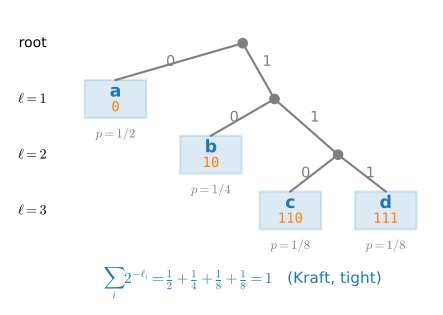
Figure 28.1.4 redraws the proof’s intervals as a binary tree. At depth \(l_i\), a codeword occupies a fraction \(2^{-l_i}\) of the available leaves. Thus shorter codewords consume a larger fraction of the code tree.
Proposition (entropy bounds the code length). Every prefix-free binary code for \(P\) has expected length \(E[l] \geq H_2(P)\) (entropy in bits), and the Shannon code with lengths \(l_i = \lceil \log_2 (1/p_i) \rceil\) is prefix-free and achieves \(E[l] < H_2(P) + 1\).
Proof. For the lower bound, let \(Z = \sum_i 2^{-l_i} \leq 1\) (Kraft) and define the distribution \(q_i = 2^{-l_i}/Z\), the one implied by the code lengths. Then \(l_i = -\log_2 q_i - \log_2 Z\), so
\[ E[l] = \sum_i p_i l_i = -\sum_i p_i \log_2 q_i - \log_2 Z = H_2(P) + D_{\textrm{KL}}^{(2)}(P \| Q) - \log_2 Z \geq H_2(P), \]
since the KL term is non-negative by Gibbs and \(-\log_2 Z \geq 0\) (the superscript \((2)\) marks base-\(2\) logs, here and in \(\textrm{CE}_2\) below). For the upper bound, the Shannon lengths satisfy \(2^{-l_i} = 2^{-\lceil \log_2(1/p_i)\rceil} \leq p_i\), so they pass Kraft’s test (\(\sum_i 2^{-l_i} \leq \sum_i p_i = 1\)) and a prefix code with these lengths exists; and \(l_i < \log_2(1/p_i) + 1\) gives \(E[l] < H_2(P) + 1\). \(\blacksquare\)
Thus entropy determines the optimal expected length to within one bit. This is the source-coding part of Shannon’s theorem, and the one-bit slack can be driven to zero by coding long blocks of symbols at once (Cover and Thomas 1999). The same proof also identifies the role of KL. If a code is designed for a distribution \(Q\), assigning approximately \(-\log_2 q_i\) bits to symbol \(i\), its expected length on data from \(P\) is
\[ -\sum_i p_i \log_2 q_i = \textrm{CE}_2(P, Q) = H_2(P) + D_{\textrm{KL}}^{(2)}(P\|Q). \]
Cross-entropy is therefore the expected length under a code based on \(Q\), and KL is the excess expected length relative to a code matched to \(P\). The same statement in nats differs by the factor \(\ln 2\).
The bound is tight enough to see in a four-line example. Take \(P = (\tfrac{1}{2}, \tfrac{1}{4}, \tfrac{1}{8}, \tfrac{1}{8})\), whose probabilities are exact powers of two, so the Shannon code wastes nothing; a codebook built for the uniform distribution instead spends \(2\) bits on every symbol.
p = [1/2, 1/4, 1/8, 1/8]
lengths = [math.ceil(math.log2(1 / p_i)) for p_i in p]
kraft = sum(2 ** -l for l in lengths)
avg_len = sum(p_i * l for p_i, l in zip(p, lengths))
h_bits = -sum(p_i * math.log2(p_i) for p_i in p)

q = [1/4] * 4   # the wrong codebook, built as if the data were uniform
lengths_q = [math.ceil(math.log2(1 / q_i)) for q_i in q]
avg_len_q = sum(p_i * l for p_i, l in zip(p, lengths_q))
kl_bits = sum(p_i * math.log2(p_i / q_i) for p_i, q_i in zip(p, q))

print(f'Shannon lengths {lengths}, Kraft sum = {kraft}')
print(f'E[l] = {avg_len} bits = H(P) = {h_bits} bits: no waste')
print(f'uniform codebook: {avg_len_q} bits = H + KL = {h_bits + kl_bits} bits')
Shannon lengths [1, 2, 3, 3], Kraft sum = 1.0
E[l] = 1.75 bits = H(P) = 1.75 bits: no waste
uniform codebook: 2.0 bits = H + KL = 2.0 bitsA possible Shannon code here is \(0,\, 10,\, 110,\, 111\), exactly the tree of Figure 28.1.4; check that it is prefix-free and that its lengths \(1, 2, 3, 3\) are the ones computed above.
28.1.3.2 From Symbol Codes to Arithmetic Coding
The Shannon code is optimal only up to that “\(+1\)”, and the leak is real: the ceiling in \(l_i = \lceil \log_2(1/p_i) \rceil\) rounds a fraction of a bit up to a whole bit, once per symbol. For a skewed source the rounding dominates the expected length. A symbol of probability \(0.9\) carries only \(-\log_2 0.9 \approx 0.15\) bits of surprisal, yet no binary codeword is shorter than one bit, so a symbol-by-symbol code overpays more than sixfold on the most common symbol it ever transmits.
The fix is to stop coding symbols and code the whole message. Arithmetic coding (Rissanen 1976; Witten et al. 1987) runs the Kraft proof’s dyadic-interval picture in reverse. Maintain a current interval, initially \([0, 1)\). To encode the next symbol, partition the current interval into one slice per possible symbol, with lengths proportional to the model’s conditional probabilities, and shrink to the slice of the symbol actually observed. After the message \(x_1, \ldots, x_N\) the interval has width
\[ w = \prod_{i=1}^N q(x_i \mid x_{<i}), \]
and it identifies the message: a decoder replaying the same model recovers each symbol in turn by watching which slice the transmitted number falls into. All that remains is to name a point of the final interval in binary, and the dyadic intervals of the Kraft proof do it: any interval of width \(w\) contains a dyadic interval of length \(2^{-l}\) with \(l = \lceil \log_2(1/w) \rceil + 1\), because \(2^{-l} \leq w/2\), so some multiple of \(2^{-l}\) falls in the interval’s left half and the dyadic interval of length \(2^{-l}\) starting there fits inside; that dyadic interval’s binary address is the codeword. The total length is therefore
\[ l \;<\; \sum_{i=1}^N \log_2 \frac{1}{q(x_i \mid x_{<i})} + 2, \]
the message’s total surprisal under the model plus at most two bits: the ceiling is paid once per message, not once per symbol. A ten-line demonstration (interval narrowing on a skewed source, then the two bit counts) makes the gap vivid.
msg = 'aaaaaaaaba'                    # nine a's, one b
q = {'a': 0.9, 'b': 0.1}              # a simple i.i.d. character model

lo, hi = 0.0, 1.0
for ch in msg:                        # narrow to the observed symbol's slice
    width = hi - lo
    if ch == 'a':                     # 'a' owns the left 90% of the interval
        hi = lo + width * q['a']
    else:                             # 'b' owns the right 10%
        lo = lo + width * q['a']

prod_q = math.prod(q[ch] for ch in msg)
surprisal = -math.log2(prod_q)                     # the floor, in bits
arith_bits = math.ceil(surprisal) + 1              # one interval, one ceiling
shannon_bits = sum(math.ceil(math.log2(1 / q[ch])) for ch in msg)

print(f'final width = {hi - lo:.6e}, prod of probs = {prod_q:.6e}')
print(f'total surprisal = {surprisal:.2f} bits')
print(f'arithmetic code: {arith_bits} bits, symbol-by-symbol Shannon code: '
      f'{shannon_bits} bits')
final width = 3.874205e-02, prod of probs = 3.874205e-02
total surprisal = 4.69 bits
arithmetic code: 6 bits, symbol-by-symbol Shannon code: 13 bitsThe final interval width equals the product of the per-symbol probabilities, as the construction promises, and the bookkeeping lands exactly where the theory says: the message’s surprisal is \(4.69\) bits, the arithmetic code spends \(6\) bits (the floor plus the once-per-message rounding), and the symbol-by-symbol Shannon code spends \(13\) bits, because it pays the ceiling’s rounded-up whole bit on each of the nine cheap a’s. On long messages the two-bit overhead vanishes into the total and the arithmetic code sits on the surprisal floor.
Notice what the construction never required: the model need not be i.i.d. Any conditional next-symbol distribution \(q(\cdot \mid x_{<i})\) works, because encoder and decoder both condition on the already-processed prefix. An autoregressive language model therefore supplies the probability model for a lossless arithmetic coder. If encoder and decoder share the tokenizer, model, and finite-precision probability implementation, the ideal code length for a document is its total surprisal plus fewer than two bits. The model’s token cross-entropy times the token count estimates that code length; a file format also carries framing and does not include the cost of distributing the model. Delétang et al. (2023) drive an arithmetic coder with an LLM’s next-token probabilities and compress text better than gzip. Thus minimizing cross-entropy improves the code length available to such a coder.
How well can any compressor do on a real source such as English text? For a stationary source \(X_1, X_2, \ldots\) (one whose statistics do not drift with position), the entropy rate
\[ H_{\textrm{rate}} = \lim_{n \to \infty} \frac{1}{n} H(X_1, \ldots, X_n) = \lim_{n \to \infty} H(X_n \mid X_{n-1}, \ldots, X_1) \tag{28.1.8}\]
is the per-symbol generalization of entropy. That the two limits exist and agree for stationary sources is a theorem we grant (Cover and Thomas 1999); the second limit is the average surprisal of the next symbol given unlimited context (conditional entropy is developed in Section 28.3), and \(H_{\textrm{rate}}\) is the floor on the expected code length per symbol of any lossless code, as \(H\) is for i.i.d. symbols. Dependence lowers the floor (conditioning reduces entropy), so a source with memory compresses better than its letter frequencies suggest: Shannon estimated the entropy rate of printed English at roughly one bit per character (Shannon 1951), far below the \(\log_2 27 \approx 4.75\) bits of uniformly random letters and spaces.
28.1.3.3 Typical Sequences and the Source-Coding Theorem
The entropy bound above concerns an expected code length. A stronger statement explains what a typical long message looks like. Let \(X_1,\ldots,X_n\) be i.i.d. draws from a finite-alphabet distribution \(P\). The probability of the realized block is \(P(X_{1:n})=\prod_i p(X_i)\), so its surprisal per symbol is a sample mean:
\[ -\frac{1}{n}\log P(X_{1:n}) =\frac{1}{n}\sum_{i=1}^n -\log p(X_i) \xrightarrow{P} H(P). \tag{28.1.9}\]
This is the asymptotic equipartition property (AEP): with probability approaching one, a long draw belongs to a typical set in which every block has probability approximately \(e^{-nH}\). Because the typical set carries almost all the probability, it must contain approximately \(e^{nH}\) blocks. The full space may have \(k^n\) possible strings, but a source uses only an exponentially smaller effective subset when \(H<\log k\).
This counting picture is the operational core of Shannon’s source-coding theorem (Shannon 1948; Cover and Thomas 1999). Encode typical blocks by their index using about \(nH\) nats (or \(nH_2\) bits), and handle the vanishing atypical set separately: rates just above entropy are achievable with failure probability tending to zero. Conversely, fewer than about \(e^{nH}\) codewords cannot name almost all typical blocks, so rates below entropy cannot be reliable. For stationary ergodic sources the entropy rate Equation 28.1.8 replaces \(H\).
For a Bernoulli source the counting claim can be checked exactly, because strings with the same number of ones share one probability. The cell groups the \(2^{200}\) binary strings of length \(n=200\) by their count of ones, declares a string typical when its surprisal is within \(0.1\) bit per symbol of \(H\), and adds up exactly how many strings are typical and how much probability they carry.
import numpy as onp
n, p = 200, 0.3
k = onp.arange(n + 1)
log_fact = onp.concatenate([[0.0], onp.cumsum(onp.log(onp.arange(1, n + 1)))])
log_count = log_fact[n] - log_fact[k] - log_fact[n - k]     # log #strings, k ones
prob_k = onp.exp(log_count + k * onp.log(p) + (n - k) * onp.log(1 - p))
h2 = -(p * onp.log2(p) + (1 - p) * onp.log2(1 - p))
bits_per_symbol = -(k * onp.log2(p) + (n - k) * onp.log2(1 - p)) / n
typical = onp.abs(bits_per_symbol - h2) < 0.1

m = log_count[typical].max()
log2_typical = (m + onp.log(onp.exp(log_count[typical] - m).sum())) / onp.log(2)
print(f'entropy H = {h2:.3f} bits/symbol, so nH = {n * h2:.0f} bits')
print(f'typical strings: 2^{log2_typical:.1f} of all 2^{n}')
print(f'probability they carry: {prob_k[typical].sum():.4f}')
entropy H = 0.881 bits/symbol, so nH = 176 bits
typical strings: 2^188.8 of all 2^200
probability they carry: 0.9893A vanishing fraction of the strings contains almost all of the probability: about \(2^{nH}\) of the \(2^n\), missing some \(24\) orders of magnitude of the count. Indexing only those strings is the compressor, and \(nH\) bits is the length of the index.
28.1.3.4 Lossy Compression and Rate–Distortion
Lossless recovery is often unnecessary. An image codec may change pixels slightly, and a learned representation may deliberately discard nuisance detail. Choose a distortion measure \(d(x,\hat x)\) and allow average distortion at most \(D\). The rate–distortion function is
\[ R(D)=\inf_{p(\hat x\mid x):\;E[d(X,\hat X)]\le D} I(X;\hat X). \tag{28.1.10}\]
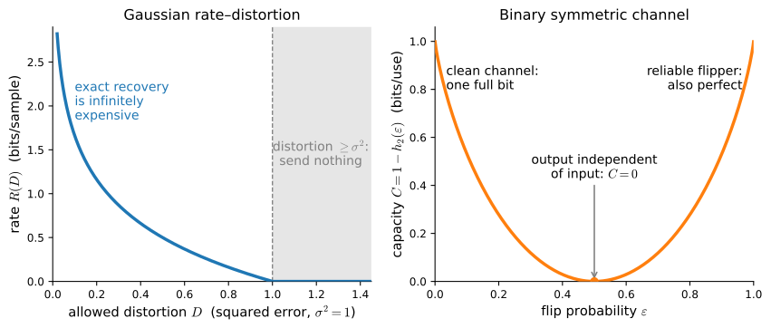
It is the smallest information rate a representation can retain while meeting the distortion budget. A stricter budget costs more bits; relaxing \(D\) lowers the rate. For a Gaussian source \(X\sim\mathcal N(0,\sigma^2)\) under squared error,
\[ R(D)=\frac12\log\frac{\sigma^2}{D} \quad (0<D<\sigma^2), \qquad R(D)=0\quad(D\ge\sigma^2), \]
in nats per sample. The left panel of Figure 28.1.5 plots it: bits buy reconstruction quality at a rate that explodes as \(D\to0\) and drops to zero once the allowed distortion exceeds the source variance — at that point transmitting nothing and reconstructing the mean is already good enough. This curve is a useful benchmark for learned compression: reconstruction losses measure distortion, while quantized latents and entropy models determine rate. Objectives of the form \(D+\beta R\) select one supporting point of the trade-off — geometrically, the point where the curve has slope \(-1/\beta\). Autoencoders and variational bottlenecks use approximations to these two terms; they do not evade the trade-off by learning the codec.
28.1.3.5 Noisy Channels and Capacity
Compression asks how few bits describe a source; communication asks how many bits survive a noisy channel. A memoryless channel is a conditional distribution \(p(y\mid x)\), whose capacity is
\[ C=\max_{p(x)} I(X;Y), \tag{28.1.11}\]
where the maximization chooses the input distribution best matched to the channel. Shannon’s noisy-channel coding theorem says that long block codes can make decoding error arbitrarily small at every rate below \(C\), while rates above \(C\) cannot be made reliable (Shannon 1948; Cover and Thomas 1999). For a binary symmetric channel that flips each bit independently with probability \(\varepsilon\), the uniform input is optimal and
\[ C=1-h_2(\varepsilon)\quad\text{bits per channel use}, \]
where \(h_2\) is binary entropy. The right panel of Figure 28.1.5 plots this curve, and it rewards a moment’s reading. At \(\varepsilon=0\) one bit survives per use. At \(\varepsilon=1/2\) the output is independent of the input and capacity is zero — no code, however clever, gets anything through. And at \(\varepsilon=1\) capacity is back to one bit: a channel that always lies is as good as one that always tells the truth, because the receiver can flip every bit. What destroys information is not corruption but unpredictability.
The same mutual-information lens applies when a representation passes through noise, quantization, dropout, or a bandwidth bottleneck. Data processing limits what later layers can recover, while coding or redundancy determines how close a designed system comes to the limit.
28.1.3.6 Perplexity
Language models are evaluated by exactly the quantity this section has been studying: the per-token cross-entropy of held-out text, \(\textrm{CE} = -\tfrac{1}{N}\sum_{i=1}^N \log q(x_i \mid x_{<i})\) nats, where \(q\) is the model’s predicted next-token distribution. The community exponentiates it and calls the result perplexity (Jelinek et al. 1977):
\[ \textrm{PPL} = \exp(\textrm{CE}) = \exp\!\Big(-\frac{1}{N}\sum_{i=1}^N \log q(x_i \mid x_{<i})\Big) = \Big(\prod_{i=1}^N q(x_i \mid x_{<i})\Big)^{-1/N}, \]
the inverse geometric mean of the probabilities the model assigned to what occurred next. Exponentiating gives an interpretation: a model that is uniformly undecided among \(V\) tokens at every step has \(\textrm{CE} = \ln V\) and hence \(\textrm{PPL} = V\), so a perplexity of, say, \(20\) means the model is, on average, as uncertain as if it were choosing uniformly among \(20\) tokens: an effective branching factor. A perfect model of a deterministic sequence has perplexity \(1\), and the floor is \(\textrm{PPL} \geq e^{H}\), where \(H\) is the entropy rate Equation 28.1.8 of the language itself, the per-token cost of its irreducible randomness (Gibbs applied to each next-token prediction, averaged, plus the entropy-rate limit granted above). Because \(\textrm{PPL} = b^{\textrm{CE}_b}\) for any log base \(b\), perplexity is also the rare information-theoretic quantity with no unit ambiguity: nats and bits give the same number (Exercise 7).
A five-token toy stream makes the bookkeeping concrete.
q_tok = [0.2, 0.1, 0.4, 0.25, 0.05]   # model prob. of each observed token
nll = [-math.log(q_i) for q_i in q_tok]
mean_nll = sum(nll) / len(nll)

print(f'per-token NLL (nats): {[round(v, 3) for v in nll]}')
print(f'mean NLL = {mean_nll:.4f} nats, perplexity = {math.exp(mean_nll):.2f}')
per-token NLL (nats): [1.609, 2.303, 0.916, 1.386, 2.996]
mean NLL = 1.8421 nats, perplexity = 6.31A mean of \(\approx 1.84\) nats per token corresponds to a perplexity of \(\approx 6.3\): this model is as confused as a uniform choice among six or so tokens. The geometric mean penalizes confident mistakes: the single \(0.05\) contributes \(3.0\) nats, as much as several good predictions combined. Perplexity in Section 8.3 and the Transformer chapters is this number.
Empirical studies have fitted held-out cross-entropy by power laws in model size, data, and training compute over substantial observed ranges (Kaplan et al. 2020; Hoffmann et al. 2022). Such fits can support planning within a studied regime, but their fitted irreducible term is not an identified entropy rate of natural language. Nor does a generic power law imply that each constant multiple of compute removes a constant fraction of the remaining loss; that interpretation describes exponential decay. Per-token quantities also depend on the tokenizer, so perplexities are directly comparable only under a shared tokenization and evaluation protocol. Bits per character or byte can improve cross-tokenizer comparability when text normalization is held fixed.
28.1.4 Modern Uses
Two modern training techniques follow directly from these identities; both are corollaries of Gibbs’ inequality.
28.1.4.1 Learning by Compression: Minimum Description Length
Likelihood measures the bits needed to encode data after a model is shared. Model selection must also account for sharing the model. The minimum description length (MDL) principle chooses the hypothesis that gives the shortest complete code,
\[ \hat h_{\textrm{MDL}} =\mathop{\mathrm{argmin}}_h \bigl[L(h)+L(\mathcal D\mid h)\bigr]. \tag{28.1.12}\]
The second term is usually a negative log-likelihood; the first pays for model complexity. A highly flexible model may compress the training residuals while losing overall because its parameters or structure are expensive to describe. This is Occam’s razor in operational units rather than a parameter-count slogan.
The connection to Bayes is close: choosing \(L(h)=-\log P(h)\) and \(L(\mathcal D\mid h)=-\log P(\mathcal D\mid h)\) gives the MAP objective. A one-part Bayesian code instead uses the marginal likelihood \(-\log\int P(\mathcal D\mid\theta)P(\theta)\,d\theta\), averaging rather than plugging in one parameter. For real-valued neural weights, a literal two-part code also needs a quantization precision and a concrete coder; counting parameters alone is not a description length. MDL is therefore a disciplined way to compare complete predictive codes, not an automatic theorem that every compressed network generalizes.
28.1.4.2 Label Smoothing
A classifier trained on one-hot targets is asked to assign probability \(1\) to the true class, which a softmax can approach only by driving the true class’s logit infinitely far above the rest. The result is overconfident models and ever-growing weights. Label smoothing (Szegedy et al. 2016) replaces the one-hot target \(\mathbf{e}_y\) with a mixture that reserves a small probability \(\epsilon\) for the other classes:
\[ \mathbf{p}^\epsilon = (1 - \epsilon)\, \mathbf{e}_y + \frac{\epsilon}{k}\, \mathbf{1}, \]
i.e., target probability \(1 - \epsilon + \epsilon/k\) for the true class and \(\epsilon/k\) for each of the other \(k - 1\). The training loss is the ordinary cross-entropy \(\textrm{CE}(\mathbf{p}^\epsilon, \mathbf{q})\) to this softened target. What prediction minimizes the smoothed loss?
Proposition (the optimal smoothed prediction). Over all probability vectors \(\mathbf{q}\), the cross-entropy \(\textrm{CE}(\mathbf{p}^\epsilon, \mathbf{q})\) is minimized uniquely at \(\mathbf{q}^* = \mathbf{p}^\epsilon\), where it equals \(H(\mathbf{p}^\epsilon)\).
Proof. By Equation 28.1.7, \(\textrm{CE}(\mathbf{p}^\epsilon, \mathbf{q}) = H(\mathbf{p}^\epsilon) + D_{\textrm{KL}}(\mathbf{p}^\epsilon \| \mathbf{q})\). The first term does not depend on \(\mathbf{q}\), and by Gibbs’ inequality the second is non-negative and zero iff \(\mathbf{q} = \mathbf{p}^\epsilon\). \(\blacksquare\)
So the optimum is no longer at infinity: the model is asked to predict \(1 - \epsilon + \epsilon/k\) on the true class, which a softmax reaches with the finite logit gap
\[ z_y - z_j = \log\frac{1 - \epsilon + \epsilon/k}{\epsilon/k} = \log\!\Big(1 + \frac{k(1-\epsilon)}{\epsilon}\Big) \]
between the true class and each other class. For \(k = 10\) classes and \(\epsilon = 0.1\) the gap is \(\ln 91 \approx 4.51\), a concrete, attainable target instead of a runaway one. (A logit difference is a log-odds ratio, so we leave it unitless rather than calling it nats.) The loss at the optimum is the (nonzero) entropy \(H(\mathbf{p}^\epsilon)\), which is why a label-smoothed loss curve plateaus above zero even when the model is doing what the softened target requests. The following calculation checks both numbers:
k, eps = 10, 0.1
p_eps = [1 - eps + eps / k] + [eps / k] * (k - 1)

gap = math.log(p_eps[0] / p_eps[1])              # optimal logit gap
h_p_eps = -sum(t * math.log(t) for t in p_eps)   # CE at the optimum q* = p_eps

z = [10.0] + [0.0] * (k - 1)                     # an overconfident prediction
z_norm = sum(math.exp(v) for v in z)
q_conf = [math.exp(v) / z_norm for v in z]
ce_conf = -sum(t * math.log(s) for t, s in zip(p_eps, q_conf))

print(f'optimal logit gap = ln(91) = {gap:.4f}')
print(f'CE at q* = H(p_eps) = {h_p_eps:.4f} nats')
print(f'CE at the overconfident q = {ce_conf:.4f} nats')
optimal logit gap = ln(91) = 4.5109
CE at q* = H(p_eps) = 0.5003 nats
CE at the overconfident q = 0.9004 natsThe overconfident prediction (logit gap \(10\)) is worse under the smoothed target than the calibrated one: label smoothing penalizes the very behavior that one-hot targets demand.
28.1.4.3 Knowledge Distillation
Knowledge distillation (Hinton et al. 2015) trains a small student network to imitate a large teacher, transferring the teacher’s full distribution over wrong answers rather than its argmax alone (a “2” that looks somewhat like a “7” is valuable information). Because a trained teacher’s softmax is nearly one-hot, both distributions are first softened with a temperature \(T\):
\[ p_j^{(T)} = \mathrm{softmax}(\mathbf{z}^{\textrm{tea}}/T)_j, \qquad q_j^{(T)} = \mathrm{softmax}(\mathbf{z}^{\textrm{stu}}/T)_j, \]
and the distillation loss is the KL divergence between the softened distributions, scaled by \(T^2\):
\[ \mathcal{L}_{\textrm{distill}} = T^2\, D_{\textrm{KL}}\big(\mathbf{p}^{(T)} \,\|\, \mathbf{q}^{(T)}\big). \]
Where does the \(T^2\) come from? Differentiate the KL term with respect to a student logit. Since only \(-\sum_j p_j^{(T)} \log q_j^{(T)}\) depends on the student, and the derivative of a log-softmax at temperature \(T\) is the usual softmax-minus-target expression scaled by \(1/T\),
\[ \frac{\partial}{\partial z^{\textrm{stu}}_j} D_{\textrm{KL}}\big(\mathbf{p}^{(T)} \| \mathbf{q}^{(T)}\big) = \frac{1}{T}\big(q_j^{(T)} - p_j^{(T)}\big). \]
For large \(T\) the softened distributions flatten toward uniform, \(\mathrm{softmax}(\mathbf{z}/T)_j \approx \tfrac{1}{k}\big(1 + (z_j - \bar z)/T\big)\) with \(\bar z\) the mean logit, so the difference \(q_j^{(T)} - p_j^{(T)}\) itself shrinks like \(1/T\) and the gradient like \(1/T^2\):
\[ \frac{1}{T}\big(q_j^{(T)} - p_j^{(T)}\big) \;\approx\; \frac{1}{k\,T^2}\Big(\big(z^{\textrm{stu}}_j - \bar z^{\textrm{stu}}\big) - \big(z^{\textrm{tea}}_j - \bar z^{\textrm{tea}}\big)\Big). \]
Multiplying the loss by \(T^2\) therefore keeps the gradient magnitude roughly constant as the temperature is tuned, so \(T\) can be chosen for the quality of the transferred soft targets without silently rescaling the learning rate against any hard-label loss it is mixed with. The following example verifies both claims numerically: the closed-form gradient matches autograd, and \(T^2\) times the gradient approaches the limit above instead of vanishing.
z_tea = torch.tensor([5.0, 2.0, -1.0])

for T in (1.0, 2.0, 5.0, 10.0):
    z_stu = torch.tensor([3.0, 3.0, 0.0], requires_grad=True)
    p, q = torch.softmax(z_tea / T, 0), torch.softmax(z_stu / T, 0)
    kl = torch.sum(p * (torch.log(p) - torch.log(q)))
    grad, = torch.autograd.grad(kl, z_stu)
    closed = (q - p).detach() / T
    err = (grad - closed).abs().max().item()
    print(f'T={T:4.1f}  |autograd - closed| = {err:.1e}  '
          f'T^2 grad = {[round(g, 3) for g in (T**2 * grad).tolist()]}')
T= 1.0 |autograd - closed| = 0.0e+00 T^2 grad = [-0.462, 0.441, 0.022]
T= 2.0 |autograd - closed| = 1.5e-08 T^2 grad = [-0.672, 0.549, 0.123]
T= 5.0 |autograd - closed| = 1.9e-09 T^2 grad = [-0.741, 0.478, 0.263]
T=10.0 |autograd - closed| = 4.7e-10 T^2 grad = [-0.719, 0.413, 0.306]z_tea = tf.constant([5.0, 2.0, -1.0])
z_stu = tf.Variable([3.0, 3.0, 0.0])
for T in (1.0, 2.0, 5.0, 10.0):
with tf.GradientTape() as tape:
p, q = tf.nn.softmax(z_tea / T), tf.nn.softmax(z_stu / T)
kl = tf.reduce_sum(p * (tf.math.log(p) - tf.math.log(q)))
grad = tape.gradient(kl, z_stu)
closed = (q - p) / T
err = float(tf.reduce_max(tf.abs(grad - closed)).numpy())
print(f'T={T:4.1f} |autograd - closed| = {err:.1e} '
f'T^2 grad = {[round(g, 3) for g in (T**2 * grad).numpy().tolist()]}')T= 1.0 |autograd - closed| = 0.0e+00 T^2 grad = [-0.462, 0.441, 0.022]
T= 2.0 |autograd - closed| = 1.5e-08 T^2 grad = [-0.672, 0.549, 0.123]
T= 5.0 |autograd - closed| = 2.8e-09 T^2 grad = [-0.741, 0.478, 0.263]
T=10.0 |autograd - closed| = 1.2e-09 T^2 grad = [-0.719, 0.413, 0.306]z_tea = jnp.array([5.0, 2.0, -1.0])
z_stu = jnp.array([3.0, 3.0, 0.0])
def distill_kl(z_stu, T):
p, q = jax.nn.softmax(z_tea / T), jax.nn.softmax(z_stu / T)
return jnp.sum(p * (jnp.log(p) - jnp.log(q)))
for T in (1.0, 2.0, 5.0, 10.0):
grad = jax.grad(distill_kl)(z_stu, T)
closed = (jax.nn.softmax(z_stu / T) - jax.nn.softmax(z_tea / T)) / T
err = jnp.abs(grad - closed).max().item()
print(f'T={T:4.1f} |autograd - closed| = {err:.1e} '
f'T^2 grad = {[round(g, 3) for g in (T**2 * grad).tolist()]}')T= 1.0 |autograd - closed| = 6.0e-08 T^2 grad = [-0.462, 0.441, 0.022]
T= 2.0 |autograd - closed| = 1.9e-09 T^2 grad = [-0.672, 0.549, 0.123]
T= 5.0 |autograd - closed| = 0.0e+00 T^2 grad = [-0.741, 0.478, 0.263]
T=10.0 |autograd - closed| = 3.5e-09 T^2 grad = [-0.719, 0.413, 0.306]z_tea = np.array([5.0, 2.0, -1.0])
z_stu = np.array([3.0, 3.0, 0.0])
z_stu.attach_grad()
for T in (1.0, 2.0, 5.0, 10.0):
with autograd.record():
p, q = npx.softmax(z_tea / T), npx.softmax(z_stu / T)
kl = np.sum(p * (np.log(p) - np.log(q)))
kl.backward()
closed = (npx.softmax(z_stu / T) - npx.softmax(z_tea / T)) / T
err = float(np.abs(z_stu.grad - closed).max())
print(f'T={T:4.1f} |autograd - closed| = {err:.1e} '
f'T^2 grad = {[round(g, 3) for g in (T**2 * z_stu.grad).tolist()]}')T= 1.0 |autograd - closed| = 0.0e+00 T^2 grad = [-0.462, 0.441, 0.022]
T= 2.0 |autograd - closed| = 3.0e-08 T^2 grad = [-0.672, 0.549, 0.123]
T= 5.0 |autograd - closed| = 2.8e-09 T^2 grad = [-0.741, 0.478, 0.263]
T=10.0 |autograd - closed| = 9.3e-10 T^2 grad = [-0.719, 0.413, 0.306][22:56:51] /home/smola/mxnet/src/base.cc:48: GPU context requested, but no GPUs found.The closed form matches autograd to floating-point precision at every temperature. The raw gradient decays like \(1/T^2\), while the \(T^2\)-scaled gradient stays order-one: its \(T \to \infty\) limit is \(\tfrac{1}{k}\big((\mathbf{z}^{\textrm{stu}} - \bar z^{\textrm{stu}}) - (\mathbf{z}^{\textrm{tea}} - \bar z^{\textrm{tea}})\big) = (-0.667, 0.333, 0.333)\) here, but the convergence is \(O(1/T)\) and still visibly incomplete in the table: the \(T = 10\) row reads \((-0.719, 0.413, 0.306)\), and the first component even overshoots its limit on the way. The scale-matching holds regardless, and that is what the \(T^2\) factor was designed for. As \(T \to 1\) the loss reduces to the ordinary KL (and, with a one-hot teacher, to the ordinary cross-entropy loss), recovering standard training as a special case.
28.1.4.4 Relations Among the Objectives
Maximum likelihood, empirical cross-entropy minimization, and KL projection of the empirical distribution onto the model family are equivalent objectives (Section 27.3.2.1). Their coding interpretation is an expected description length, while perplexity is the corresponding exponentiated per-token loss. Label smoothing and distillation replace the hard empirical target with different target distributions. The next section extends KL to other discrepancies between distributions (Section 28.2); the final section applies KL to a joint distribution and the product of its marginals to obtain mutual information (Section 28.3).
28.1.5 Summary
- Self-information \(I(x) = -\log p(x)\) measures the surprise of an outcome; entropy \(H(P) = -E_{x\sim P}[\log p(x)]\) is the average surprise of a distribution. We measure both in nats (natural log); bits differ by a factor of \(\ln 2\).
- On \(k\) outcomes, \(0 \leq H(P) \leq \log k\), with the maximum exactly at the uniform distribution (Jensen). Differential entropy \(h\) of continuous variables is not coordinate-invariant and can be negative, one reason deep learning prefers relative quantities; under fixed mean and variance it is maximized by the Gaussian (Section 28.1.2.3).
- The KL divergence \(D_{\textrm{KL}}(P\|Q) = E_{x\sim P}[\log p(x)/q(x)]\) is asymmetric and, by Gibbs’ inequality, non-negative with equality iff \(P = Q\).
- Cross-entropy decomposes as \(\textrm{CE}(P, Q) = H(P) + D_{\textrm{KL}}(P\|Q)\). Minimizing it in \(Q\) is minimizing KL, and on empirical data it is maximum likelihood (Section 27.3.2.1).
- As a scoring rule, the cross-entropy loss (the log score) is strictly proper: at population risk, a model class containing the truth is uniquely minimized by the true conditional probabilities. Finite data, restricted models, and distribution shift can still produce miscalibration.
- In the coding view, entropy is the optimal expected code length (Kraft inequality + Shannon code) and KL is the extra bits per symbol from coding with the wrong distribution.
- Arithmetic coding removes the symbol code’s per-symbol rounding: with a shared model and coder, a whole message costs its total surprisal plus at most two bits. An autoregressive model supplies the probabilities for that lossless code; its cross-entropy times the token count is the model code length before file-format overhead. The entropy rate is the per-symbol floor for any such code. The AEP explains this floor by showing that almost all length-\(n\) messages occupy a typical set of size about \(e^{nH}\).
- Rate–distortion gives the smallest retained information compatible with a distortion budget, while channel capacity \(C=\max_{p(x)}I(X;Y)\) gives the largest reliable communication rate through noise.
- Minimum description length selects a complete code for model plus data; negative log-likelihood is only the data-given-model part.
- Perplexity \(\textrm{PPL} = \exp(\textrm{CE})\) is the exponentiated per-token cross-entropy of a language model: an effective branching factor, independent of the log base. Empirically it falls as a power law in parameters, data, and compute, and it is comparable only under a shared tokenizer.
- Label smoothing and knowledge distillation are corollaries of the same identities: the smoothed target makes the cross-entropy optimum finite and equal to the deliberately softened target; it does not by itself guarantee calibration to the original data distribution, and the \(T^2\) factor on the distillation KL keeps gradients scale-matched across temperatures.
28.1.6 Exercises
- Verify the card-deck numbers from the first subsection: the four reports carry \(0\), \(\ln 4\), \(\ln 52\), and \(\ln 52!\) nats. Use Stirling’s approximation to estimate \(\ln 52!\) and check it against the exact value.
- Give a second proof that the uniform distribution maximizes entropy on \(k\) outcomes, this time from Gibbs’ inequality: show that \(D_{\textrm{KL}}(P \,\|\, U) = \log k - H(P)\) for the uniform \(U\), and conclude.
- Compute the entropy of the following data sources:
- Suppose that you are watching the output generated by a monkey at a typewriter that hits any of the \(44\) keys uniformly at random. How many nats (and bits) of randomness per character do you observe?
- Unhappy with the monkey, you replace it with a drunk typesetter that picks a random word out of a vocabulary of \(2{,}000\) words, with an average word length of \(4.5\) letters. How many nats per character now?
- Still unhappy, you replace the typesetter with a language model that achieves a per-word perplexity of \(15\). How many nats per character does that correspond to?
- Derive the closed form Equation 28.1.5 for the KL divergence between two univariate Gaussians by writing \(E_{x\sim P}[\log p(x) - \log q(x)]\) and using \(E_{x \sim P}[x] = \mu_1\), \(E_{x\sim P}[(x-\mu_1)^2] = \sigma_1^2\).
- Show that self-information is unique up to scale: if a continuous, decreasing function \(I(p)\) on \((0, 1]\) satisfies \(I(1) = 0\) and \(I(p_1 p_2) = I(p_1) + I(p_2)\) for all \(p_1, p_2\), then \(I(p) = -c \log p\) for some constant \(c > 0\).
- A scoring rule \(S(\mathbf{q}, y)\) is strictly proper if the expected penalty \(E_{y \sim \mathbf{p}}[S(\mathbf{q}, y)]\) is uniquely minimized at \(\mathbf{q} = \mathbf{p}\). Prove from Gibbs’ inequality that the log score \(S(\mathbf{q}, y) = -\log q_y\) is strictly proper. Then prove that the Brier score \(S(\mathbf{q}, y) = \sum_j (q_j - \mathbf{1}[j = y])^2\) is strictly proper too, by showing that its expected penalty exceeds the truthful reporter’s by exactly \(\|\mathbf{q} - \mathbf{p}\|^2\) (Gneiting and Raftery 2007).
- Show that perplexity does not depend on the log base: if \(\textrm{CE}_b\) denotes the per-token cross-entropy in base-\(b\) units, then \(b^{\textrm{CE}_b}\) is the same for every \(b\). Then compute the perplexity of a model whose per-token cross-entropy is \(\ln 5\) nats.
- For label smoothing with \(k\) classes and smoothing parameter \(\epsilon\), derive the optimal prediction \(\mathbf{q}^*\) and the optimal logit gap, and evaluate the gap for \(k = 1000\), \(\epsilon = 0.1\). What happens to the gap as \(\epsilon \to 0\), and why does that recover the one-hot pathology?
- For the distillation loss, derive the gradient formula \(\partial D_{\textrm{KL}}(\mathbf{p}^{(T)} \| \mathbf{q}^{(T)}) / \partial z^{\textrm{stu}}_j = (q_j^{(T)} - p_j^{(T)})/T\), and show that as \(T \to \infty\) the \(T^2\)-scaled gradient tends to \(\tfrac{1}{k}\big((z^{\textrm{stu}}_j - \bar z^{\textrm{stu}}) - (z^{\textrm{tea}}_j - \bar z^{\textrm{tea}})\big)\). What does the loss reduce to at \(T = 1\) with a one-hot teacher?