24.2 Matrices as Linear Maps

In Section 24.1 we read \(\mathbf{A}\mathbf{x}\) by rows: entry \(i\) is the dot product of row \(i\) with \(\mathbf{x}\), one hyperplane test per output, so that a 10-class softmax layer is a set of 10 normal vectors. That reading says what a matrix computes for one input. It does not say what the matrix does to all inputs at once, and in particular whether its effect can be undone.

The question arises as soon as a layer is narrower than its input. A fully connected layer from the 784 pixels of a Fashion-MNIST image to 256 features is a \(256 \times 784\) matrix. Its output holds fewer numbers than its input. By a count we make precise below, it sends at least \(784 - 256 = 528\) independent input directions to zero, so different images produce the same features before any nonlinearity sees them. A square matrix may or may not lose information. The running matrix of this chapter, \(\mathbf{A} = \left(\begin{smallmatrix}1 & 2\\ -1 & 3\end{smallmatrix}\right)\), sends the vector \((2, -1)\) to \((0, -5)\), and another matrix sends \((0, -5)\) back to \((2, -1)\). That matrix undoes \(\mathbf{A}\) on every input, so \(\mathbf{A}\) loses nothing. The matrix \(\mathbf{B} = \left(\begin{smallmatrix}2 & 1\\ 4 & 2\end{smallmatrix}\right)\) sends both \((1, 1)\) and \((0, 3)\) to \((3, 6)\). Seeing the output \((3, 6)\), we cannot tell which of the two inputs we started from, so no matrix can bring it back.

Whether a map can be undone decides whether a layer discards information, whether a linear system has one solution or many, and how a probability density changes under a change of variables. We answer the question by reading a matrix through its columns. Column \(j\) is the image of the \(j\)-th coordinate axis, and these images determine the whole map. The number of linearly independent columns, the rank, tells how many input dimensions survive. The signed volume of the image of the unit cube, the determinant, tells in one number whether any dimension is lost. We work first in two dimensions, where every statement is a picture, and then in \(n\) dimensions.

import numpy as np

import numpy as np

import numpy as np

import numpy as np

24.2.1 Linear Maps

24.2.1.1 Columns as Images of the Axes

A matrix acts on infinitely many inputs, yet it is a finite table of numbers. To see how the table determines every output, take a \(2 \times 2\) matrix \(\mathbf{A}\) with entries \(a, b, c, d\) (in the \(2 \times 2\) formulas of this section, \(d\) is an entry, not a dimension) and apply it to \(\mathbf{x} = (x, y)\). Collecting the terms that multiply \(x\) and those that multiply \(y\) gives

\[ \mathbf{A}\mathbf{x} = \begin{bmatrix}a & b \\ c & d\end{bmatrix}\begin{bmatrix}x \\ y\end{bmatrix} = \begin{bmatrix}ax+by\\ cx+dy\end{bmatrix} = x\begin{bmatrix}a \\ c\end{bmatrix} + y\begin{bmatrix}b \\d\end{bmatrix} = x\,\mathbf{A}\mathbf{e}_1 + y\,\mathbf{A}\mathbf{e}_2. \]

So \(\mathbf{A}\mathbf{x}\) is a weighted sum of the two columns of \(\mathbf{A}\), with the entries of \(\mathbf{x}\) as weights, and the columns are the images of the standard basis vectors \(\mathbf{e}_1 = (1, 0)\) and \(\mathbf{e}_2 = (0, 1)\). The images of two vectors fix the image of every vector.

For the running matrix (\(a = 1\), \(b = 2\), \(c = -1\), \(d = 3\)) the axes go to \(\mathbf{A}\mathbf{e}_1 = (1, -1)\) and \(\mathbf{A}\mathbf{e}_2 = (2, 3)\). The input \(\mathbf{v} = (2, -1)\) is \(2\mathbf{e}_1 - \mathbf{e}_2\), so its image is the same combination of the columns,

\[ \mathbf{A}\mathbf{v} = 2\,(1, -1) - (2, 3) = (0, -5). \]

The row view gives the same numbers: \((1, 2)\cdot(2, -1) = 0\) and \((-1, 3)\cdot(2, -1) = -5\). Both readings compute the same product. This section uses the columns, because they show where the map sends the whole plane. Figure 24.2.1 draws it: the unit square spanned by \(\mathbf{e}_1\) and \(\mathbf{e}_2\) goes to the parallelogram spanned by the two columns, and the grid point \(\mathbf{v}\) goes to the grid point \(\mathbf{A}\mathbf{v}\) of the image grid.

Figure 24.2.1: The running matrix \(\mathbf{A} = \left(\begin{smallmatrix}1 & 2\\ -1 & 3\end{smallmatrix}\right)\) acting on the plane. (a) The input grid, the shaded unit square, the basis vectors and the input \(\mathbf{v} = (2, -1)\). (b) Its image: \(\mathbf{e}_1\) goes to \((1, -1)\), \(\mathbf{e}_2\) to \((2, 3)\), and \(\mathbf{v}\) to \((0, -5)\). The grid is carried along: lines stay lines, the origin stays put, and equally spaced points stay equally spaced. The shaded square goes to the shaded parallelogram, whose area is the subject of the determinant. Panel (b) is drawn at one third the scale of (a).

We check the three images in code.

A = np.array([[1.0, 2.0], [-1.0, 3.0]])
e1, e2 = np.eye(2)
v = np.array([2.0, -1.0])
A @ e1, A @ e2, A @ v

(array([ 1., -1.]), array([2., 3.]), array([ 0., -5.]))

The output lists the two columns of \(\mathbf{A}\) and the image \((0, -5)\).

The same holds for every size. An \(m \times n\) matrix takes vectors with \(n\) entries to vectors with \(m\) entries, so it is a map from \(\mathbb{R}^n\) to \(\mathbb{R}^m\), and this map is linear:

\[ \mathbf{A}(\alpha\mathbf{x} + \beta\mathbf{y}) = \alpha\,\mathbf{A}\mathbf{x} + \beta\,\mathbf{A}\mathbf{y} \quad \textrm{for all } \mathbf{x}, \mathbf{y} \in \mathbb{R}^n \textrm{ and } \alpha, \beta \in \mathbb{R}. \]

In words, the image of a weighted sum is the same weighted sum of the images. Writing \(\mathbf{x} = \sum_j x_j \mathbf{e}_j\) gives \(\mathbf{A}\mathbf{x} = \sum_j x_j\,\mathbf{A}\mathbf{e}_j\), and multiplying by the column vector \(\mathbf{e}_j\) selects column \(j\). Conversely, every map \(f : \mathbb{R}^n \to \mathbb{R}^m\) with this linearity property is given by a matrix, the one whose column \(j\) is \(f(\mathbf{e}_j)\), because \(f(\mathbf{x}) = f(\sum_j x_j\mathbf{e}_j) = \sum_j x_j f(\mathbf{e}_j)\). Linear maps from \(\mathbb{R}^n\) to \(\mathbb{R}^m\) and \(m \times n\) matrices are therefore the same objects.

Linearity also keeps the grid of Figure 24.2.1 a grid. The points \(\mathbf{p} + t\mathbf{u}\) of a line go to \(\mathbf{A}\mathbf{p} + t\,\mathbf{A}\mathbf{u}\), again a line (or a single point, when \(\mathbf{A}\mathbf{u} = \mathbf{0}\)) traversed at a constant rate. The origin stays put, \(\mathbf{A}\mathbf{0} = \mathbf{0}\).

Nothing requires the matrix to be square. A \(2 \times 3\) matrix sends \(\mathbb{R}^3\) into the span of its three columns, which fills the whole output plane only when some two of the columns are not multiples of one another. A \(3 \times 2\) matrix sends the plane into \(\mathbb{R}^3\), and its outputs form a plane through the origin, a line, or the origin alone, depending on its two columns. Every fully connected layer of a neural network is such a map between spaces of different dimensions, followed by a nonlinearity.

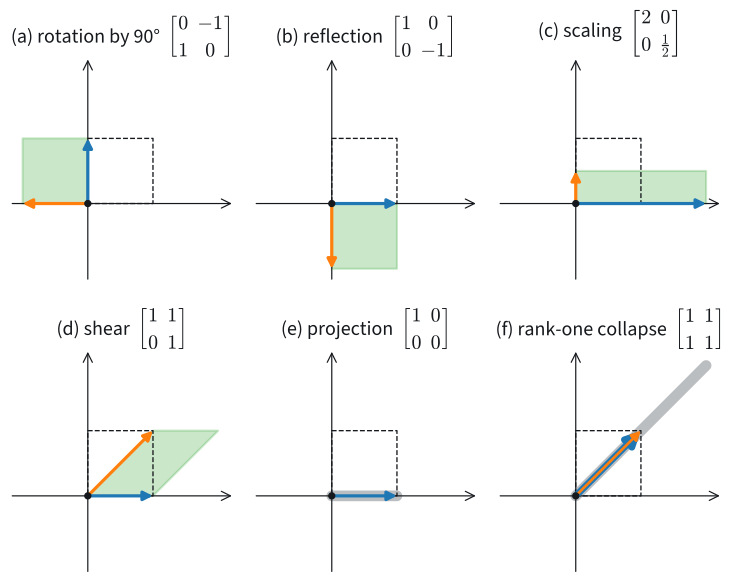
Within these rules, matrices act on the plane in different ways. Figure 24.2.2 shows six of them, each as the image of the unit square, with the two columns drawn. The rotation by \(90^\circ\) sends \(\mathbf{e}_1\) to \(\mathbf{e}_2\) and \(\mathbf{e}_2\) to \(-\mathbf{e}_1\), so its columns are \((0, 1)\) and \((-1, 0)\). The shear keeps \(\mathbf{e}_1\) fixed and tilts \(\mathbf{e}_2\) to \((1, 1)\), so it slides each horizontal line sideways by its height. The last two panels lose a dimension: the whole square, and with it the whole plane, lands on a line.

Figure 24.2.2: Six things a \(2 \times 2\) matrix can do to the unit square (dashed). In each panel the columns, drawn as arrows, are the images of \(\mathbf{e}_1\) (blue) and \(\mathbf{e}_2\) (orange), and the shaded region is the image of the square. Panels (e) and (f) send the plane onto a line; in (f) both columns are \((1, 1)\).

A matrix records where the axes go. One familiar operation is not of this kind: the translation \(\mathbf{x} \mapsto \mathbf{x} + \mathbf{c}\) with \(\mathbf{c} \neq \mathbf{0}\) moves the origin, so it is not linear. A layer \(\mathbf{W}\mathbf{x} + \mathbf{b}\) is a linear map followed by such a shift.

24.2.1.2 Composition

Two linear layers in a row, with no nonlinearity between them, form a single map. Which matrix represents it? Take the rotation by \(90^\circ\) and the shear of Figure 24.2.2,

\[ \mathbf{R}_{90} = \begin{bmatrix}0 & -1\\ 1 & 0\end{bmatrix}, \qquad \mathbf{S} = \begin{bmatrix}1 & 1\\ 0 & 1\end{bmatrix}. \]

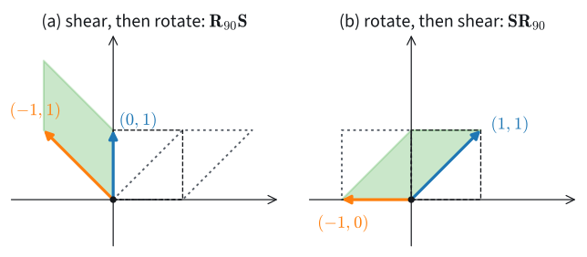
Shearing first sends \(\mathbf{e}_1\) to \((1, 0)\), and rotating that gives \((0, 1)\); shearing sends \(\mathbf{e}_2\) to \((1, 1)\), and rotating that gives \((-1, 1)\). The composite map “shear, then rotate” therefore has the columns \((0, 1)\) and \((-1, 1)\). In the other order, rotating sends \(\mathbf{e}_1\) to \((0, 1)\), which the shear moves to \((1, 1)\), and \(\mathbf{e}_2\) to \((-1, 0)\), which the shear leaves alone. The two composites are

\[ \textrm{shear, then rotate: }\begin{bmatrix}0 & -1\\ 1 & 1\end{bmatrix}, \qquad \textrm{rotate, then shear: }\begin{bmatrix}1 & -1\\ 1 & 0\end{bmatrix}. \]

The two orders give different maps, as Figure 24.2.3 shows.

Figure 24.2.3: The order of composition matters. (a) The shear \(\mathbf{S}\) (dotted outline: the square after the shear), then the rotation \(\mathbf{R}_{90}\); the product is \(\mathbf{R}_{90}\mathbf{S}\). (b) The rotation (dotted: the square after the rotation), then the shear; the product is \(\mathbf{S}\mathbf{R}_{90}\). The labels give the images of \(\mathbf{e}_1\) (blue) and \(\mathbf{e}_2\) (orange). A product of matrices is read from right to left.

The matrix product computes such composites. For any two matrices \(\mathbf{A}\) and \(\mathbf{B}\) whose sizes fit, apply \(\mathbf{B}\) to \(\mathbf{v}\), then \(\mathbf{A}\) to the result, and write out entry \(i\):

\[ \bigl(\mathbf{A}(\mathbf{B}\mathbf{v})\bigr)_i = \sum_j a_{ij} (\mathbf{B}\mathbf{v})_j = \sum_j \sum_k a_{ij} b_{jk} v_k = \sum_k \Bigl(\sum_j a_{ij} b_{jk}\Bigr) v_k = \bigl((\mathbf{A}\mathbf{B})\mathbf{v}\bigr)_i. \tag{24.2.1}\]

Applying the two maps in turn is the same as applying the single matrix \(\mathbf{A}\mathbf{B}\), whose entry \((i, k)\) is row \(i\) of \(\mathbf{A}\) times column \(k\) of \(\mathbf{B}\). The product \(\mathbf{A}\mathbf{B}\) means “\(\mathbf{B}\) first, then \(\mathbf{A}\)”, read from right to left like \(f(g(x))\). Taking \(\mathbf{v} = \mathbf{e}_j\) in Equation 24.2.1 shows that column \(j\) of \(\mathbf{A}\mathbf{B}\) is \(\mathbf{A}\mathbf{b}_j\), the image under \(\mathbf{A}\) of column \(j\) of \(\mathbf{B}\). We use this fact for the determinant.

Composition explains the multiplication rule. The product is row-times-column because that is what the composite of two linear maps computes. It is associative, \((\mathbf{A}\mathbf{B})\mathbf{C} = \mathbf{A}(\mathbf{B}\mathbf{C})\), because composing functions is associative: both sides apply \(\mathbf{C}\), then \(\mathbf{B}\), then \(\mathbf{A}\). And it is not commutative, because composing two functions in the other order generally gives another function. The code computes the two products and their action on \(\mathbf{e}_1\).

R90 = np.array([[0.0, -1.0], [1.0, 0.0]])  # rotation by 90 degrees
S = np.array([[1.0, 1.0], [0.0, 1.0]])     # shear
print(R90 @ S)
print(S @ R90)
(R90 @ S) @ e1, (S @ R90) @ e1

[[ 0. -1.]
 [ 1.  1.]]
[[ 1. -1.]
 [ 1.  0.]]

(array([0., 1.]), array([1., 1.]))

The printed matrices are the two composites above, and \(\mathbf{e}_1\) goes to \((0, 1)\) in one order and to \((1, 1)\) in the other. Some pairs do commute. Two rotations of the plane commute, since rotating by \(\phi\) and then by \(\psi\) rotates by \(\phi + \psi\) in either order. Two diagonal matrices commute, since each scales the axes independently. Exercise 5 finds every matrix that commutes with \(\mathbf{R}_{90}\).

24.2.1.3 Orthogonal Matrices

Some maps move space rigidly: every length, and every angle between two embedding vectors, comes out unchanged. Which matrices do this? The rotation by an angle \(\phi\) sends \(\mathbf{e}_1\) to \((\cos\phi, \sin\phi)\) and \(\mathbf{e}_2\) to \((-\sin\phi, \cos\phi)\), so its matrix is

\[ \mathbf{R}_\phi = \begin{bmatrix}\cos\phi & -\sin\phi\\ \sin\phi & \cos\phi\end{bmatrix}. \]

Its columns have length \(\sqrt{\cos^2\phi + \sin^2\phi} = 1\) and dot product \(-\cos\phi\sin\phi + \sin\phi\cos\phi = 0\). Since entry \((i, j)\) of \(\mathbf{R}_\phi^\top\mathbf{R}_\phi\) is the dot product of columns \(i\) and \(j\), these three numbers say \(\mathbf{R}_\phi^\top\mathbf{R}_\phi = \mathbf{I}\). With \(\phi = 90^\circ\) we get \(\mathbf{R}_{90}\), which sends \((3, 2)\) to \((-2, 3)\); both have length \(\sqrt{13}\). The reflection \(\operatorname{diag}(1, -1)\) in the \(x\)-axis sends \((3, 2)\) to \((3, -2)\), again of length \(\sqrt{13}\), and applying it twice gives the identity, so it is its own inverse.

A square matrix \(\mathbf{Q}\) is orthogonal when its columns are orthonormal, that is, unit vectors that are pairwise perpendicular. Written with the dot products of the columns, the condition is

\[ \mathbf{Q}^\top\mathbf{Q} = \mathbf{I}. \]

The rotations \(\mathbf{R}_\phi\) and the reflection \(\operatorname{diag}(1, -1)\) are orthogonal. Columns that are only perpendicular are not enough: \(\operatorname{diag}(1, 10)\) has perpendicular columns of lengths \(1\) and \(10\), and it changes the angle between \((1, 1)\) and \((1, -1)\) from \(90^\circ\) to \(\arccos(-99/101) \approx 169^\circ\) (1). A rectangular \(n \times k\) matrix with orthonormal columns, \(k < n\), also satisfies \(\mathbf{Q}^\top\mathbf{Q} = \mathbf{I}_k\) and preserves lengths, but it maps \(\mathbb{R}^k\) into the larger space \(\mathbb{R}^n\) and has no two-sided inverse (Section 24.2.2.3). The name “orthogonal matrix” is reserved for the square case.

An orthogonal map preserves every dot product,

\[ (\mathbf{Q}\mathbf{x})\cdot(\mathbf{Q}\mathbf{y}) = (\mathbf{Q}\mathbf{x})^\top(\mathbf{Q}\mathbf{y}) = \mathbf{x}^\top\mathbf{Q}^\top\mathbf{Q}\,\mathbf{y} = \mathbf{x}^\top\mathbf{y} = \mathbf{x}\cdot\mathbf{y}. \]

Taking \(\mathbf{y} = \mathbf{x}\) shows \(\|\mathbf{Q}\mathbf{x}\| = \|\mathbf{x}\|\), and since the angle between two vectors is computed from their dot product and their lengths, angles are preserved too. For \(\mathbf{R}_{90}\), \(\mathbf{x} = (3, 2)\) and \(\mathbf{y} = (1, 0)\), we get \(\mathbf{x}\cdot\mathbf{y} = 3\) and \((-2, 3)\cdot(0, 1) = 3\). Rotating every embedding by the same orthogonal matrix therefore leaves all their cosine similarities unchanged. The code checks the definition, the lengths and the dot product.

x, y = np.array([3.0, 2.0]), np.array([1.0, 0.0])
F = np.diag([1.0, -1.0])                   # reflection in the x-axis
print(np.allclose(R90.T @ R90, np.eye(2)), np.allclose(F.T @ F, np.eye(2)))
print(R90 @ x, np.linalg.norm(R90 @ x), np.linalg.norm(x))
(R90 @ x) @ (R90 @ y), x @ y

True True
[-2.  3.] 3.605551275463989 3.605551275463989

(np.float64(3.0), np.float64(3.0))

True True
[-2.  3.] 3.605551275463989 3.605551275463989

(np.float64(3.0), np.float64(3.0))

True True
[-2.  3.] 3.605551275463989 3.605551275463989

(np.float64(3.0), np.float64(3.0))

True True
[-2.  3.] 3.605551275463989 3.605551275463989

(3.0, 3.0)

Both matrices pass the test \(\mathbf{Q}^\top\mathbf{Q} = \mathbf{I}\), the rotated vector has the length \(\sqrt{13} \approx 3.606\) of the original, and the dot product \(3\) is unchanged.

The condition \(\mathbf{Q}^\top\mathbf{Q} = \mathbf{I}\) says that \(\mathbf{Q}^\top\) undoes \(\mathbf{Q}\) when applied after it. For a square \(\mathbf{Q}\), it also undoes \(\mathbf{Q}\) when applied before it, \(\mathbf{Q}\mathbf{Q}^\top = \mathbf{I}\). The rows are then orthonormal too, and \(\mathbf{Q}^{-1} = \mathbf{Q}^\top\). This follows from a general fact about square matrices, shown in Section 24.2.2.3.

In the plane, rotations and reflections are the only orthogonal matrices. The first column of an orthogonal \(2 \times 2\) matrix is a unit vector, so it is \((\cos\phi, \sin\phi)\) for some angle \(\phi\). The second column is a unit vector perpendicular to it, and there are two of these, \(\pm(-\sin\phi, \cos\phi)\). With the plus sign the matrix is the rotation \(\mathbf{R}_\phi\). With the minus sign it is \(\mathbf{R}_\phi\operatorname{diag}(1, -1)\), the reflection in the \(x\)-axis followed by a rotation, which is a reflection in a line through the origin. Every orthogonal \(2 \times 2\) matrix is a rotation or a reflection, and Section 24.2.3.3 shows that the sign of the determinant tells the two kinds apart.

24.2.2 Rank and Invertibility

24.2.2.1 Column Space and Null Space

Which outputs can a matrix produce, and which inputs does it erase? The matrix

\[ \mathbf{B} = \begin{bmatrix} 2 & 1 \\ 4 & 2 \end{bmatrix} \]

has the columns \(\mathbf{b}_1 = (2, 4)\) and \(\mathbf{b}_2 = (1, 2)\), and \(\mathbf{b}_1 = 2\mathbf{b}_2\). Every output is a combination of the columns, and such a combination collapses to a multiple of one column,

\[ a_1\mathbf{b}_1 + a_2\mathbf{b}_2 = (2a_1 + a_2)\,\mathbf{b}_2. \]

All outputs of \(\mathbf{B}\) therefore lie on the line through \((1, 2)\), the line \(y = 2x\). Distinct inputs collide on that line: \(\mathbf{B}(1, 1) = (3, 6)\) and \(\mathbf{B}(0, 3) = (3, 6)\). By linearity their difference \((1, -2)\) goes to the difference of the outputs, \(\mathbf{B}(1, -2) = \mathbf{0}\). The row view shows why: both rows, \((2, 1)\) and \((4, 2)\), are perpendicular to \((1, -2)\), so both hyperplane tests return zero. Figure 24.2.4 shows the two lines.

Figure 24.2.4: The matrix \(\mathbf{B} = \left(\begin{smallmatrix}2 & 1\\ 4 & 2\end{smallmatrix}\right)\) collapsing the plane. (a) The input plane, with the null-space line through \((1, -2)\) dashed and perpendicular to the row direction \((2, 1)\), and three marked inputs: \(\mathbf{x}_1 = (1, 1)\), \(\mathbf{x}_2 = (0, 3)\), and \(\mathbf{x}_3 = (1, -2)\) on the null-space line. (b) The image plane, at the same scale: every output lies on the column space, the line \(y = 2x\) spanned by the columns \(\mathbf{b}_1\) and \(\mathbf{b}_2\); \(\mathbf{x}_1\) and \(\mathbf{x}_2\) land on the same point \((3, 6)\), and \(\mathbf{x}_3\) lands on the origin. Because distinct inputs have the same image, no inverse exists.

We confirm the three images.

B = np.array([[2.0, 1.0], [4.0, 2.0]])
B @ np.array([1.0, 1.0]), B @ np.array([0.0, 3.0]), B @ np.array([1.0, -2.0])

(array([3., 6.]), array([3., 6.]), array([0., 0.]))

The first two outputs agree, and \((1, -2)\) goes to zero.

Two subspaces attach to every \(m \times n\) matrix \(\mathbf{A}\). The column space \(\operatorname{col}\mathbf{A}\) is the span of the columns. Since \(\mathbf{A}\mathbf{x}\) is the combination of the columns with weights \(x_1, \ldots, x_n\), the column space is the set of all outputs. The null space is the set of inputs sent to zero,

\[ \ker\mathbf{A} = \{\mathbf{x} \in \mathbb{R}^n : \mathbf{A}\mathbf{x} = \mathbf{0}\}. \]

It is a subspace: if \(\mathbf{A}\mathbf{x} = \mathbf{A}\mathbf{y} = \mathbf{0}\), then \(\mathbf{A}(\alpha\mathbf{x} + \beta\mathbf{y}) = \alpha\mathbf{A}\mathbf{x} + \beta\mathbf{A}\mathbf{y} = \mathbf{0}\). For \(\mathbf{B}\) the column space is the line \(y = 2x\) and the null space is the line through \((1, -2)\). These are two different lines, with slopes \(2\) and \(-2\), so the figure keeps their roles apart.

Three general facts follow the example.

The null space consists of the inputs perpendicular to every row. This is the row view: \((\mathbf{A}\mathbf{x})_i\) is the dot product of row \(i\) with \(\mathbf{x}\), and all of these vanish if and only if \(\mathbf{x}\) is perpendicular to all rows.
The columns are linearly dependent if and only if the null space contains a nonzero vector. Vectors are linearly dependent, as in Section 24.1, when some combination of them with coefficients not all zero gives \(\mathbf{0}\). A dependence \(\sum_j x_j\mathbf{a}_j = \mathbf{0}\) among the columns \(\mathbf{a}_j\) of \(\mathbf{A}\) says \(\mathbf{A}\mathbf{x} = \mathbf{0}\), so its coefficients form a nonzero null vector, and the converse reads the same equation backwards. For \(\mathbf{B}\), the dependence \(\mathbf{b}_1 - 2\mathbf{b}_2 = \mathbf{0}\) has the coefficients \((1, -2)\).
Two inputs have the same output if and only if they differ by a null vector, because \(\mathbf{A}\mathbf{x} = \mathbf{A}\mathbf{y}\) means \(\mathbf{A}(\mathbf{x} - \mathbf{y}) = \mathbf{0}\). The inputs that \(\mathbf{B}\) sends to \((3, 6)\) form the line \((1, 1) + t(1, -2)\), which contains \((0, 3)\) at \(t = -1\). A nonzero null vector therefore means that no inverse can exist.

24.2.2.2 Rank

How many input dimensions survive the map? The rank of a matrix is the dimension of its column space, equivalently the largest number of linearly independent columns:

\[ \operatorname{rank}\mathbf{A} = \dim\operatorname{col}\mathbf{A}. \]

The matrix \(\mathbf{B}\) has rank one: its two columns are dependent, and each column is nonzero. As a larger example, consider

\[ \mathbf{C} = \begin{bmatrix} 1& 3 & 0 & -1 & 0 \\ -1 & 0 & 1 & 1 & -1 \\ 0 & 3 & 1 & 0 & -1 \\ 2 & 3 & -1 & -2 & 1 \end{bmatrix}, \]

which has rank two: the first two columns are linearly independent, while each of the \(\binom{5}{3} = 10\) collections of three columns is linearly dependent (2).

The dimensions that survive and the dimensions sent to zero add up to the number of input dimensions.

Proposition (rank–nullity). For an \(m \times n\) matrix \(\mathbf{A}\),

\[ \operatorname{rank}\mathbf{A} + \dim\ker\mathbf{A} = n. \tag{24.2.2}\]

Proof. Choose a basis \(\mathbf{w}_1, \ldots, \mathbf{w}_k\) of the null space and extend it to a basis \(\mathbf{w}_1, \ldots, \mathbf{w}_k, \mathbf{u}_1, \ldots, \mathbf{u}_{n-k}\) of \(\mathbb{R}^n\). The images \(\mathbf{A}\mathbf{u}_1, \ldots, \mathbf{A}\mathbf{u}_{n-k}\) span the column space, since every input is a combination of the basis vectors and the \(\mathbf{w}_i\) contribute nothing. They are also independent: if \(\sum_i c_i \mathbf{A}\mathbf{u}_i = \mathbf{0}\), then \(\sum_i c_i \mathbf{u}_i\) lies in the null space, hence is a combination of the \(\mathbf{w}_j\), which is impossible within a basis unless every \(c_i = 0\). So the column space has dimension \(n - k\). \(\blacksquare\)

Of the \(n\) input dimensions, \(\dim\ker\mathbf{A}\) are sent to zero and \(\operatorname{rank}\mathbf{A}\) remain in the image. For \(\mathbf{B}\) the count is \(1 + 1 = 2\). For \(\mathbf{C}\) it is \(2 + 3 = 5\): the vectors \((3, -1, 3, 0, 0)\), \((1, 0, 0, 1, 0)\) and \((0, 0, 1, 0, 1)\) are independent null vectors, and rank–nullity leaves no room for a fourth. For the \(256 \times 784\) layer of the introduction, the rank is at most \(256\), the number of output coordinates, so the null space has dimension at least \(784 - 256 = 528\). The code checks the counts for \(\mathbf{B}\) and \(\mathbf{C}\).

C = np.array([[1, 3, 0, -1, 0], [-1, 0, 1, 1, -1],
              [0, 3, 1, 0, -1], [2, 3, -1, -2, 1]], dtype=float)
Z = np.array([[3, -1, 3, 0, 0], [1, 0, 0, 1, 0],
              [0, 0, 1, 0, 1]], dtype=float).T   # candidate null vectors
rank_C, rank_Z = np.linalg.matrix_rank(C), np.linalg.matrix_rank(Z)
np.linalg.matrix_rank(B), rank_C, np.abs(C @ Z).max(), rank_Z, rank_C + rank_Z

(np.int64(1), np.int64(2), np.float64(0.0), np.int64(3), np.int64(5))

(np.int64(1), np.int64(2), np.float64(0.0), np.int64(3), np.int64(5))

(np.int64(1), np.int64(2), np.float64(0.0), np.int64(3), np.int64(5))

(1, 2, 0.0, 3, 5)

The ranks of \(\mathbf{B}\) and \(\mathbf{C}\) are \(1\) and \(2\), the three candidates are sent to zero and are independent (rank \(3\)), and \(2 + 3 = 5\).

The same matrix can be read by rows. Its row rank, the largest number of linearly independent rows, counts the independent hyperplane tests the matrix performs. For \(\mathbf{C}\), row 3 is row 1 plus row 2 and row 4 is row 1 minus row 2, so the row rank is two, the same as the rank. The two ranks agree for every matrix.

Proposition (row rank equals column rank). For every matrix \(\mathbf{A}\), the largest number of linearly independent rows equals the largest number of linearly independent columns.

Proof. Let \(r = \operatorname{rank}\mathbf{A}\) and put a basis of \(\operatorname{col}\mathbf{A}\) into the columns of an \(m \times r\) matrix \(\mathbf{G}\). We factor \(\mathbf{A}\) through this basis. Every column of \(\mathbf{A}\) is a combination of the columns of \(\mathbf{G}\), and writing the coefficients for column \(j\) into column \(j\) of an \(r \times n\) matrix \(\mathbf{H}\) gives

\[ \mathbf{A} = \mathbf{G}\mathbf{H}. \tag{24.2.3}\]

Now read the same product by rows. Row \(i\) of \(\mathbf{A}\) is \(\sum_k g_{ik}\,(\textrm{row } k \textrm{ of } \mathbf{H})\), so all rows of \(\mathbf{A}\) lie in the span of the \(r\) rows of \(\mathbf{H}\), and the row rank is at most \(r\). Applying the same argument to \(\mathbf{A}^\top\), whose columns are the rows of \(\mathbf{A}\), shows that the column rank is at most the row rank. \(\blacksquare\)

The factorization says that a matrix of rank \(r\) first computes \(r\) numbers from its input (the map \(\mathbf{H}\)) and then spreads them over the \(m\) outputs (the map \(\mathbf{G}\)).

Finding the rank by checking subsets of columns takes exponentially long. By hand one uses elimination. The routine np.linalg.matrix_rank instead counts the nonzero singular values, numbers defined later in this chapter. Rank is not a continuous function of the entries. The matrix \(\left(\begin{smallmatrix}1 & 10^8\\ 0 & 1\end{smallmatrix}\right)\) has rank two, and a change of \(10^{-8}\) in one entry brings it to rank one (Section 24.2.5).

24.2.2.3 Inverses

Given an output \(\mathbf{A}\mathbf{x}\), can we recover the input \(\mathbf{x}\)? An inverse of a square matrix \(\mathbf{A}\) is a matrix \(\mathbf{A}^{-1}\) that undoes it from both sides,

\[ \mathbf{A}^{-1}\mathbf{A} = \mathbf{A}\mathbf{A}^{-1} = \mathbf{I}, \]

where the identity matrix \(\mathbf{I}\), with ones on the diagonal and zeros elsewhere, leaves every vector unchanged. Then \(\mathbf{x} = \mathbf{A}^{-1}(\mathbf{A}\mathbf{x})\). For a \(2 \times 2\) matrix with entries \(a, b, c, d\) and \(ad - bc \neq 0\), the inverse is

\[ \mathbf{A}^{-1} = \frac{1}{ad - bc}\begin{bmatrix} d & -b \\ -c & a \end{bmatrix}. \tag{24.2.4}\]

Multiplying out confirms the formula: the matrix \(\left(\begin{smallmatrix}d & -b\\ -c & a\end{smallmatrix}\right)\) times \(\mathbf{A}\), in either order, is \((ad - bc)\,\mathbf{I}\), and dividing by \(ad - bc\) leaves \(\mathbf{I}\). The number \(ad - bc\) is the determinant of \(\mathbf{A}\), which Section 24.2.3.1 defines as a signed area. The theorem of Section 24.2.3.4 shows that the hypothesis \(ad - bc \neq 0\) is the condition for an inverse to exist. For the running matrix, \(ad - bc = 3 + 2 = 5\), and

\[ \mathbf{A}^{-1} = \frac{1}{5}\begin{bmatrix} 3 & -2 \\ 1 & 1 \end{bmatrix}, \qquad \mathbf{A}^{-1}(0, -5) = \tfrac15\,(10, -5) = (2, -1). \]

The inverse undoes the worked example of Section 24.2.1.1. The code builds \(\mathbf{A}^{-1}\) from the formula and compares it with the library solver.

a, b, c, d = A.ravel()
A_inv = np.array([[d, -b], [-c, a]]) / (a * d - b * c)
print(A_inv)
np.allclose(A_inv @ A, np.eye(2)), A_inv @ (A @ v), np.linalg.solve(A, A @ v)

[[ 0.6 -0.4]
 [ 0.2  0.2]]

(True, array([ 2., -1.]), array([ 2., -1.]))

The formula gives \(\tfrac15\left(\begin{smallmatrix}3 & -2\\ 1 & 1\end{smallmatrix}\right)\), its product with \(\mathbf{A}\) is the identity, and both the formula and np.linalg.solve recover \(\mathbf{v} = (2, -1)\) from \(\mathbf{A}\mathbf{v}\).

A left inverse and a right inverse of the same matrix always agree, so the inverse is unique. If \(\mathbf{L}\mathbf{A} = \mathbf{I}\) and \(\mathbf{A}\mathbf{R} = \mathbf{I}\), then

\[ \mathbf{L} = \mathbf{L}(\mathbf{A}\mathbf{R}) = (\mathbf{L}\mathbf{A})\mathbf{R} = \mathbf{R}, \]

with associativity in the middle step. This settles the orthogonal case of Section 24.2.1.3: \(\mathbf{Q}^\top\) is a left inverse of \(\mathbf{Q}\), so once we know that \(\mathbf{Q}\) has some right inverse, that right inverse equals \(\mathbf{Q}^\top\), and \(\mathbf{Q}\mathbf{Q}^\top = \mathbf{I}\).

When does an inverse exist? A square matrix with linearly independent columns is invertible; we state this here and prove it in Section 24.2.3.4. A matrix with a nonzero null vector has no inverse, by fact 3 above. An \(m \times n\) matrix with \(m \neq n\) has no two-sided inverse at all. Its rank is at most \(\min(m, n)\). If \(m > n\), the column space has dimension at most \(n < m\), so the matrix is not onto: some targets in \(\mathbb{R}^m\) are never hit. If \(n > m\), rank–nullity leaves a null space of dimension at least \(n - m > 0\), so the matrix is not one-to-one: some distinct inputs give the same output. The inverse runs the map backwards, and it exists when no two inputs collide and every target is hit. The singular matrix \(\mathbf{B}\) fails both tests.

24.2.2.4 Solving Linear Systems in Practice

The inverse is a tool for reasoning, but in practice we rarely compute it. To solve \(\mathbf{A}\mathbf{x} = \mathbf{b}\), prefer np.linalg.solve(A, b) to np.linalg.inv(A) @ b, for two reasons. The first is cost. solve factors \(\mathbf{A}\) once into triangular factors (an LU factorization, about \(n^3/3\) multiply–adds) and then solves two triangular systems. Forming the inverse takes about \(n^3\) multiply–adds before the product with \(\mathbf{b}\) even starts. The second is accuracy. solve is backward stable: its answer is the exact solution of a system whose entries differ from those of \(\mathbf{A}\) and \(\mathbf{b}\) only by rounding. Its residual \(\|\mathbf{A}\mathbf{x} - \mathbf{b}\|\) is therefore of the order of machine precision times \(\|\mathbf{A}\|\,\|\mathbf{x}\|\). The product inv(A) @ b carries no such guarantee, and its residual can be larger by a factor up to the condition number \(\kappa(\mathbf{A})\), a measure of how close \(\mathbf{A}\) is to a singular matrix (Section 24.4.3.2).

How close a matrix is to singular is a property of the problem, not of the method. Both methods can lose up to about \(\log_{10}\kappa(\mathbf{A})\) of the sixteen decimal digits of double precision in the solution itself. The condition number bounds this loss in the worst case; it does not predict the loss for a given right-hand side. The Hilbert matrix, with entries \(h_{ij} = 1/(i + j - 1)\), is a classical example of a nearly singular matrix. We set \(\mathbf{x} = \mathbf{1}\), compute the right-hand side \(\mathbf{b} = \mathbf{H}\mathbf{1}\) for the \(10 \times 10\) Hilbert matrix \(\mathbf{H}\), and solve for \(\mathbf{x}\) again both ways.

H = 1 / (np.arange(10)[:, None] + np.arange(10) + 1)   # Hilbert matrix
x_true = np.ones(10)
b = H @ x_true
for x in (np.linalg.solve(H, b), np.linalg.inv(H) @ b):
    print(f'residual {np.linalg.norm(H @ x - b):.1e}, '
          f'error {np.linalg.norm(x - x_true):.1e}')
np.linalg.cond(H)

residual 5.7e-16, error 2.7e-04
residual 4.8e-05, error 9.0e-03

np.float64(16024416987428.36)

residual 5.7e-16, error 2.7e-04
residual 4.8e-05, error 9.0e-03

np.float64(16024416987428.36)

residual 5.7e-16, error 2.7e-04
residual 4.8e-05, error 9.0e-03

np.float64(16024416987428.36)

residual 5.7e-16, error 2.7e-04
residual 4.8e-05, error 9.0e-03

16024416987428.36

The residual of solve is near machine precision, about \(10^{-15}\) or less, while that of inv is many orders of magnitude larger. Both solutions are wrong after the first few digits, as \(\kappa(\mathbf{H}) \approx 1.6 \cdot 10^{13}\) predicts: about a dozen of the sixteen digits are lost whichever method we use.

Sparse matrices give a further reason to avoid the inverse. A matrix with a million rows and columns but only five million nonzero entries is cheap to store, yet its inverse is typically dense, with about \(10^{12}\) nonzero entries.

24.2.3 The Determinant

24.2.3.1 Area of a Parallelogram

By how much does \(\mathbf{A}\) scale areas? In Figure 24.2.1 the unit square, with edges \(\mathbf{e}_1\) and \(\mathbf{e}_2\) and area one, goes to the parallelogram with edges \(\mathbf{a}_1 = (1, -1)\) and \(\mathbf{a}_2 = (2, 3)\) and corners \((0, 0)\), \((1, -1)\), \((3, 2)\) and \((2, 3)\). We now compute its area. The parallelogram fits in the box \([0, 3] \times [-1, 3]\) of area \(12\). The part of the box outside it consists of four right triangles, with legs \(1\) and \(1\), \(2\) and \(3\), \(1\) and \(1\), and \(2\) and \(3\), of total area \(\tfrac12 + 3 + \tfrac12 + 3 = 7\). The parallelogram has area \(12 - 7 = 5\) (Figure 24.2.5, panel (a)). The matrix multiplies the area of the unit square by five.

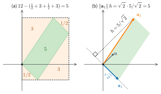
Figure 24.2.5: The image of the unit square under \(\mathbf{A}\) has area \(5\). (a) The bounding box \([0, 3] \times [-1, 3]\), of area \(12\), minus four right triangles of total area \(7\). (b) Base times height: the base \(\mathbf{a}_1 = (1, -1)\) has length \(\sqrt{2}\), the unit normal \(\mathbf{n} = (1, 1)/\sqrt{2}\) is perpendicular to it, and the height of the corner \(\mathbf{a}_2 = (2, 3)\) above the line through \(\mathbf{a}_1\) is \(\mathbf{a}_2\cdot\mathbf{n} = 5/\sqrt{2}\).

Counting triangles needs a new picture for every arrangement of the corners. Base times height works for all of them at once. Let the parallelogram have the edges \(\mathbf{u} = (a, c)\) and \(\mathbf{w} = (b, d)\), the two columns of a \(2 \times 2\) matrix with entries \(a, b, c, d\). Its base has length \(\|\mathbf{u}\|\). The vector \((-c, a)\) is \(\mathbf{u}\) rotated by \(90^\circ\), that is, \(\mathbf{R}_{90}\mathbf{u}\), so

\[ \mathbf{n} = \frac{(-c, a)}{\|\mathbf{u}\|} \]

is a unit vector perpendicular to the base. By Section 24.1, the component of \(\mathbf{w}\) along a unit vector \(\mathbf{n}\) is \(\mathbf{w}\cdot\mathbf{n}\). Here this component is the height of the parallelogram above its base, with a sign: positive when \(\mathbf{w}\) lies on the counter-clockwise side of \(\mathbf{u}\), negative on the clockwise side. Base times signed height is

\[ \|\mathbf{u}\|\,(\mathbf{w}\cdot\mathbf{n}) = \|\mathbf{u}\|\,\frac{-bc + ad}{\|\mathbf{u}\|} = ad - bc. \]

The lengths cancel, and what remains is a polynomial in the four entries. No case distinction on signs was needed. For the running matrix, \(\|\mathbf{u}\| = \sqrt{2}\), \(\mathbf{n} = (1, 1)/\sqrt{2}\), and \(\mathbf{w}\cdot\mathbf{n} = 5/\sqrt{2}\), so the signed area is \(5\), as the count gave (panel (b)). It is positive because \(\mathbf{a}_2\) lies counter-clockwise from \(\mathbf{a}_1\).

The determinant of a \(2 \times 2\) matrix is this signed area of the image of the unit square:

\[ \det\begin{bmatrix} a & b \\ c & d \end{bmatrix} = ad - bc. \tag{24.2.5}\]

Its absolute value is the factor by which the matrix scales area, and its sign records whether the images of \(\mathbf{e}_1\) and \(\mathbf{e}_2\) keep their counter-clockwise order. For \(\mathbf{A}\), \(1 \cdot 3 - 2 \cdot (-1) = 5\). Exchanging the two columns of \(\mathbf{A}\) gives \(\left(\begin{smallmatrix}2 & 1\\ 3 & -1\end{smallmatrix}\right)\), whose image is the same parallelogram with its edges in the other order, and the determinant is \(-2 - 3 = -5\). For \(\mathbf{B}\) it is \(2 \cdot 2 - 1 \cdot 4 = 0\): the square goes to the segment from \(\mathbf{0}\) to \((3, 6)\), which has no area. The code computes base times height and the library determinant of the three matrices.

u, w = A[:, 0], A[:, 1]
n = np.array([-u[1], u[0]]) / np.linalg.norm(u)   # unit normal to u
(np.linalg.norm(u) * (w @ n), np.linalg.det(A),
 np.linalg.det(A[:, ::-1]), np.linalg.det(B))

(np.float64(5.0),
 np.float64(4.999999999999999),
 np.float64(-5.000000000000001),
 np.float64(0.0))

(np.float64(5.0),
 np.float64(4.999999999999999),
 np.float64(-5.000000000000001),
 np.float64(0.0))

(np.float64(5.0),
 np.float64(4.999999999999999),
 np.float64(-5.000000000000001),
 np.float64(0.0))

(5.0, 4.999999999999999, -5.000000000000001, 0.0)

Up to rounding in the last digit, the values are \(5\), \(5\), \(-5\) and \(0\). Figure 24.2.6 shows the three cases: a positive determinant keeps the orientation, a negative one reverses it, and a zero determinant flattens the square.

Figure 24.2.6: The determinant as signed area for the three matrices of this section. The unit square (dashed) goes to the region spanned by the columns. (a) \(\mathbf{A}\), determinant \(5\): the columns keep their counter-clockwise order (curved arrow). (b) \(\mathbf{A}\) with its columns exchanged, determinant \(-5\): the same parallelogram with the orientation reversed. (c) \(\mathbf{B}\), determinant \(0\): the square collapses to a segment of the line \(y = 2x\). Panel (c) is drawn at half the scale of (a) and (b).

In two dimensions the area is zero if and only if the two edges lie on one line through the origin, that is, if and only if the columns are linearly dependent, as for \(\mathbf{B}\). The same statement in \(n\) dimensions needs the determinant of an \(n \times n\) matrix, which we construct next; it is proved in Section 24.2.3.4.

24.2.3.2 The Determinant in General

What is the signed volume of the box spanned by \(n\) vectors in \(\mathbb{R}^n\)? Rather than compute volumes in \(n\) dimensions directly, we list three properties of signed volume and let them determine the answer. Stated for the columns \(\mathbf{a}_1, \ldots, \mathbf{a}_n\) of an \(n \times n\) matrix, the determinant is

Multilinear: linear in each column separately, with the other columns held fixed. (Scaling one edge of a box scales its volume; splitting one edge as a sum splits the volume accordingly.)
Alternating: zero whenever two columns are equal. (The box then flattens into a lower-dimensional slab of zero volume.)
Normalized: \(\det \mathbf{I} = 1\). (The unit cube has volume one.)

The area \(ad - bc\) has all three properties: it is linear in \((a, c)\) and in \((b, d)\), it vanishes when \((a, c) = (b, d)\), and it is \(1\) for the identity. We show below that at most one function of the columns has the three properties, and that it must be given by the permutation formula Equation 24.2.6. Conversely, the formula does have the three properties. The proof rests on one fact, which we take from (Horn and Johnson 2012): the parity of a permutation, whether it is a product of an even or an odd number of swaps, is well defined.

Uniqueness comes in a sharper form that we use later: every function \(f\) of the columns satisfying (1) and (2) is a multiple of the determinant, \(f = f(\mathbf{I}) \cdot \det\). To see why, set \(g = f - f(\mathbf{I})\cdot\det\). Then \(g\) satisfies (1) and (2) with \(g(\mathbf{I}) = 0\), so \(g + \det\) satisfies all three properties. By uniqueness it equals \(\det\), which forces \(g = 0\).

The first consequence of the properties is that swapping two columns flips the sign of the determinant. Place the vector \(\mathbf{u}+\mathbf{w}\) in two column slots and expand by multilinearity:

\[ \begin{aligned} 0 &= \det(\ldots, \mathbf{u}+\mathbf{w}, \ldots, \mathbf{u}+\mathbf{w}, \ldots) \\ &= \det(\ldots, \mathbf{u}, \ldots, \mathbf{u}, \ldots) + \det(\ldots, \mathbf{u}, \ldots, \mathbf{w}, \ldots) + \det(\ldots, \mathbf{w}, \ldots, \mathbf{u}, \ldots) + \det(\ldots, \mathbf{w}, \ldots, \mathbf{w}, \ldots). \end{aligned} \]

The left-hand side, the first term and the last term vanish by the alternating property, which leaves

\[ \det(\ldots, \mathbf{u}, \ldots, \mathbf{w}, \ldots) = -\det(\ldots, \mathbf{w}, \ldots, \mathbf{u}, \ldots). \]

This is where the sign of the signed area comes from: exchanging two edges reverses the orientation of the box, as in panel (b) of Figure 24.2.6.

Second, the three properties pin down a formula. Expand each column in the standard basis, \(\mathbf{a}_j = \sum_i a_{ij}\,\mathbf{e}_i\), and apply multilinearity column by column. Then \(\det\mathbf{A}\) becomes a sum of terms \(a_{i_1 1} a_{i_2 2} \cdots a_{i_n n}\, \det(\mathbf{e}_{i_1}, \ldots, \mathbf{e}_{i_n})\), one for every choice of a row index in each column. Whenever two of the chosen row indices coincide, the term vanishes by the alternating property. When all are distinct, the columns \(\mathbf{e}_{i_1}, \ldots, \mathbf{e}_{i_n}\) are those of the identity matrix in another order, and repeated column swaps turn the factor into \(\pm 1\). For a \(2 \times 2\) matrix with columns \(\mathbf{a}_1 = a\,\mathbf{e}_1 + c\,\mathbf{e}_2\) and \(\mathbf{a}_2 = b\,\mathbf{e}_1 + d\,\mathbf{e}_2\), the expansion has four terms. The two with a repeated basis vector vanish, and

\[ \det(\mathbf{a}_1, \mathbf{a}_2) = ad\,\det(\mathbf{e}_1, \mathbf{e}_2) + cb\,\det(\mathbf{e}_2, \mathbf{e}_1) = ad - bc, \]

the area we computed by hand. In general the determinant is a signed sum, over all ways of picking one entry from each row and each column, of the product of the picked entries. Writing \(\sigma(j)\) for the row picked in column \(j\), this is the permutation formula

\[\det\mathbf{A} = \sum_{\sigma} \operatorname{sgn}(\sigma)\, a_{\sigma(1)1}\, a_{\sigma(2)2} \cdots a_{\sigma(n)n}, \tag{24.2.6}\]

where \(\sigma\) runs over the \(n!\) permutations of \(\{1, \ldots, n\}\) and \(\operatorname{sgn}(\sigma) = \det(\mathbf{e}_{\sigma(1)}, \ldots, \mathbf{e}_{\sigma(n)})\) is \(+1\) or \(-1\) according to whether \(\sigma\) is made of an even or an odd number of swaps. The three properties leave no other possibility, which is the uniqueness claimed above.

For hand computation the sum is organized as cofactor expansion along the first column. The terms with \(\sigma(1) = i\) all contain the factor \(a_{i1}\). What multiplies it is the determinant of the submatrix with row \(i\) and column \(1\) deleted, with the sign \((-1)^{i+1}\) that accounts for the \(i - 1\) swaps moving row \(i\) to the top. So \(\det\mathbf{A}\) splits into \(n\) smaller determinants with alternating signs. For the \(3 \times 3\) example

\[ \mathbf{M} = \begin{bmatrix} 2 & 1 & 0 \\ 1 & 3 & 1 \\ 0 & 1 & 2 \end{bmatrix} \]

the expansion along the first column reads

\[ \det \mathbf{M} = 2 \det \begin{bmatrix} 3 & 1 \\ 1 & 2 \end{bmatrix} - 1 \det \begin{bmatrix} 1 & 0 \\ 1 & 2 \end{bmatrix} + 0 \det \begin{bmatrix} 1 & 0 \\ 3 & 1 \end{bmatrix} = 2 \cdot 5 - 1 \cdot 2 + 0 = 8. \tag{24.2.7}\]

Geometrically, \(\mathbf{M}\) maps the unit cube to a box of volume \(8\). The code checks Equation 24.2.7 and two consequences of the properties: swapping two columns flips the sign, and the determinant of a triangular matrix is the product of its diagonal entries.

M = np.array([[2, 1, 0], [1, 3, 1], [0, 1, 2]])
M_swap = M[:, [1, 0, 2]]                         # first two columns swapped
T = np.array([[2, 5, 1], [0, 3, 4], [0, 0, 1]])  # upper triangular
(np.linalg.det(M),       # 8, matching the cofactor expansion
 np.linalg.det(M_swap),  # -8: a column swap flips the sign
 np.linalg.det(T))       # 6 = 2 * 3 * 1, the diagonal product

(np.float64(8.000000000000002),
 np.float64(-8.000000000000002),
 np.float64(6.0))

(np.float64(8.000000000000002),
 np.float64(-8.000000000000002),
 np.float64(6.0))

(np.float64(8.000000000000002),
 np.float64(-8.000000000000002),
 np.float64(6.0))

(8.000000000000002, -8.000000000000002, 6.0)

Up to rounding, the outputs are \(8\), \(-8\) and \(6\). The triangular rule follows from the permutation formula. Suppose \(\mathbf{T}\) is upper triangular, so \(t_{ij} = 0\) whenever \(i > j\). Each term of the permutation formula picks one entry from every column, all in distinct rows. To be nonzero, the entry picked from column \(1\) must come from row \(1\), since every lower entry vanishes. The entry from column \(2\) must then come from row \(2\), because row \(1\) is taken and rows \(3, \ldots, n\) hold zeros. Continuing across the columns, only the diagonal choice survives, and it needs no swaps, so

\[ \det \mathbf{T} = t_{11} t_{22} \cdots t_{nn}. \]

The determinant of a triangular matrix is the product of its diagonal entries. The same argument, run from column \(n\) backwards, handles lower triangular matrices.

Transposing does not change the determinant, \(\det\mathbf{A}^\top = \det\mathbf{A}\). For \(2 \times 2\) matrices, transposing swaps \(b\) and \(c\) and leaves \(ad - bc\) unchanged. In general, the permutation formula for \(\mathbf{A}^\top\) has the terms \(\operatorname{sgn}(\sigma)\prod_j a_{j\sigma(j)}\). Substituting \(j = \sigma^{-1}(i)\) rewrites the product as \(\prod_i a_{\sigma^{-1}(i)\, i}\), the term of the formula for \(\mathbf{A}\) that belongs to the permutation \(\sigma^{-1}\). As \(\sigma\) runs over all permutations so does \(\sigma^{-1}\), and \(\operatorname{sgn}(\sigma^{-1}) = \operatorname{sgn}(\sigma)\), because undoing a sequence of swaps takes the same number of swaps. The two formulas have the same terms. Consequently, everything the determinant says about columns holds for rows as well.

The permutation formula has \(n!\) terms and is never used to compute a determinant beyond tiny sizes. Libraries factor the matrix into triangular factors, as in solve, and multiply the diagonal entries of the factors, with a sign for the row exchanges, at a cost of about \(n^3/3\) multiply–adds.

24.2.3.3 Multiplicativity

If \(\mathbf{B}\) scales areas by \(\det\mathbf{B}\) and \(\mathbf{A}\) scales them by \(\det\mathbf{A}\), then the composite \(\mathbf{A}\mathbf{B}\) should scale them by the product. For the running matrix, \(\mathbf{A}^2 = \left(\begin{smallmatrix}-1 & 8\\ -4 & 7\end{smallmatrix}\right)\) and \(\det\mathbf{A}^2 = -7 + 32 = 25 = 5^2\). For the composite of Section 24.2.1.2, \(\det(\mathbf{R}_{90}\mathbf{S}) = 0 \cdot 1 - (-1) \cdot 1 = 1\), the product of \(\det\mathbf{R}_{90} = 1\) and \(\det\mathbf{S} = 1\).

The intuition comes from tiling. Cover a planar figure with small squares. A linear map sends each square to a parallelogram, and all of these parallelograms have the same area, \(|\det\mathbf{A}|\) times that of a square, because the map acts in the same way everywhere. So a linear map scales the area of every figure by the same factor \(|\det\mathbf{A}|\). Applying \(\mathbf{B}\) to a figure of area \(V\) gives the area \(|\det\mathbf{B}|\,V\), and applying \(\mathbf{A}\) next gives \(|\det\mathbf{A}|\,|\det\mathbf{B}|\,V\). The composite is a single linear map, so its own factor must be this product. The three properties turn the tiling argument into a proof, signs included.

Proposition (multiplicativity of the determinant). For square matrices \(\mathbf{A}\) and \(\mathbf{B}\) of the same size,

\[ \det(\mathbf{A}\mathbf{B}) = \det(\mathbf{A})\,\det(\mathbf{B}). \tag{24.2.8}\]

Proof. Fix \(\mathbf{A}\) and view \(D(\mathbf{B}) = \det(\mathbf{A}\mathbf{B})\) as a function of the columns of \(\mathbf{B}\) alone. By Section 24.2.1.2, column \(j\) of \(\mathbf{A}\mathbf{B}\) is \(\mathbf{A}\mathbf{b}_j\). Because \(\mathbf{A}(\cdot)\) is linear and \(\det\) is multilinear, \(D\) is multilinear in the columns of \(\mathbf{B}\). If two columns of \(\mathbf{B}\) are equal, so are the corresponding columns of \(\mathbf{A}\mathbf{B}\), and \(D(\mathbf{B}) = 0\); so \(D\) is alternating. By the scaling form of uniqueness in Section 24.2.3.2,

\[ \det(\mathbf{A}\mathbf{B}) = D(\mathbf{B}) = D(\mathbf{I})\,\det(\mathbf{B}) = \det(\mathbf{A})\,\det(\mathbf{B}). \qquad \blacksquare \]

The volume factor of a composite is the product of the volume factors. We check the examples numerically; A_inv is the inverse computed in Section 24.2.2.3 and F the reflection \(\operatorname{diag}(1, -1)\).

(np.linalg.det(A @ A), np.linalg.det(A) ** 2, np.linalg.det(R90 @ S),
 np.linalg.det(A_inv), np.linalg.det(F))

(np.float64(25.000000000000007),
 np.float64(24.999999999999993),
 np.float64(1.0),
 np.float64(0.2),
 np.float64(-1.0))

(np.float64(25.000000000000007),
 np.float64(24.999999999999993),
 np.float64(1.0),
 np.float64(0.2),
 np.float64(-1.0))

(np.float64(25.000000000000007),
 np.float64(24.999999999999993),
 np.float64(1.0),
 np.float64(0.2),
 np.float64(-1.0))

(25.000000000000007, 24.999999999999993, 1.0, 0.2, -1.0)

Up to rounding, the values are \(25\), \(25\), \(1\), \(0.2\) and \(-1\). The last two are explained by the following four consequences of Equation 24.2.8.

Determinants commute even when matrices do not. Since the two determinants are scalars, \(\det(\mathbf{A}\mathbf{B}) = \det\mathbf{A}\,\det\mathbf{B} = \det\mathbf{B}\,\det\mathbf{A} = \det(\mathbf{B}\mathbf{A})\). For the rotation and the shear, \(\mathbf{R}_{90}\mathbf{S} \neq \mathbf{S}\mathbf{R}_{90}\), but both products have determinant \(1\).
Similarity invariance. For an invertible \(\mathbf{V}\), applying consequence 1 to the pair \(\mathbf{V}\mathbf{A}\) and \(\mathbf{V}^{-1}\) gives \(\det(\mathbf{V}\mathbf{A}\mathbf{V}^{-1}) = \det(\mathbf{V}^{-1}\mathbf{V}\mathbf{A}) = \det\mathbf{A}\). The matrix \(\mathbf{V}\mathbf{A}\mathbf{V}^{-1}\) describes the map \(\mathbf{A}\) in the coordinates whose axes are the columns of \(\mathbf{V}^{-1}\), and a change of coordinates does not change the volume factor.
Inverses. If \(\mathbf{A}\) is invertible, taking \(\mathbf{B} = \mathbf{A}^{-1}\) gives \(\det\mathbf{A}\,\det\mathbf{A}^{-1} = \det\mathbf{I} = 1\). Hence an invertible matrix has \(\det\mathbf{A} \neq 0\), and \(\det\mathbf{A}^{-1} = 1/\det\mathbf{A}\); for the running matrix, \(1/5 = 0.2\).
Orthogonal matrices. Combining multiplicativity with \(\det\mathbf{Q}^\top = \det\mathbf{Q}\) and applying both to \(\mathbf{Q}^\top\mathbf{Q} = \mathbf{I}\) gives

\[ \det(\mathbf{Q})^2 = \det(\mathbf{Q}^\top)\det(\mathbf{Q}) = \det(\mathbf{Q}^\top\mathbf{Q}) = \det(\mathbf{I}) = 1, \]

so \(\det\mathbf{Q} = \pm 1\). A rigid motion leaves the size of every volume unchanged, and the sign records whether it keeps the orientation. Every rotation has \(\det\mathbf{R}_\phi = \cos^2\phi + \sin^2\phi = 1\), and the reflection \(\operatorname{diag}(1, -1)\) has determinant \(-1\). In the classification of Section 24.2.1.3, the orthogonal \(2 \times 2\) matrices with determinant \(1\) are the rotations, and those with determinant \(-1\) are the reflections.

24.2.3.4 Invertibility and the Determinant

We now have three tests for a square matrix: its columns, its rank, and its determinant. In two dimensions they agree on sight. The signed area \(ad - bc\) is zero if and only if the two edges lie on one line through the origin (or one of them is \(\mathbf{0}\)), that is, if and only if the columns are dependent. Dependent columns send the whole plane onto a line, or onto the origin if the matrix is zero, and there distinct inputs collide. The following proposition says the same in every dimension.

Proposition (invertibility and the determinant). For an \(n \times n\) matrix \(\mathbf{A}\), the following are equivalent: (i) \(\det\mathbf{A} = 0\); (ii) the columns of \(\mathbf{A}\) are linearly dependent; (iii) \(\mathbf{A}\) is not invertible.

Proof. We show (ii) \(\Rightarrow\) (i) \(\Rightarrow\) (iii) \(\Rightarrow\) (ii).

(ii) \(\Rightarrow\) (i). If the columns are dependent, one of them is a combination of the others, \(\mathbf{a}_j = \sum_{i \neq j} c_i\mathbf{a}_i\). Multilinearity in column \(j\) gives \(\det\mathbf{A} = \sum_{i \neq j} c_i\det(\ldots, \mathbf{a}_i, \ldots)\), where \(\mathbf{a}_i\) now stands in slot \(j\). Every term has two equal columns, so it vanishes by the alternating property.

(i) \(\Rightarrow\) (iii). This is consequence 3 of multiplicativity read backwards: an invertible matrix has \(\det\mathbf{A}\,\det\mathbf{A}^{-1} = 1\), so \(\det\mathbf{A} \neq 0\).

(iii) \(\Rightarrow\) (ii). We show the contrapositive: independent columns make \(\mathbf{A}\) invertible. With independent columns the null space is \(\{\mathbf{0}\}\), since a nonzero null vector would be a dependence. By rank–nullity the rank is \(n\), so the column space is an \(n\)-dimensional subspace of \(\mathbb{R}^n\), which is all of \(\mathbb{R}^n\): every target is hit. And \(\mathbf{A}\mathbf{x} = \mathbf{A}\mathbf{y}\) forces \(\mathbf{x} - \mathbf{y} \in \ker\mathbf{A} = \{\mathbf{0}\}\), so no two inputs collide. It remains to build the inverse from these two facts. Let column \(j\) of a matrix \(\mathbf{X}\) be the unique solution of \(\mathbf{A}\mathbf{x} = \mathbf{e}_j\). Then \(\mathbf{A}\mathbf{X} = \mathbf{I}\) by construction. For any \(\mathbf{x}\), \(\mathbf{A}(\mathbf{X}\mathbf{A}\mathbf{x}) = (\mathbf{A}\mathbf{X})\mathbf{A}\mathbf{x} = \mathbf{A}\mathbf{x}\), and since no two inputs collide, \(\mathbf{X}\mathbf{A}\mathbf{x} = \mathbf{x}\). So \(\mathbf{X}\mathbf{A} = \mathbf{I}\) as well, and \(\mathbf{X} = \mathbf{A}^{-1}\). \(\blacksquare\)

For the running matrix, \(\det\mathbf{A} = 5 \neq 0\), and its inverse is the matrix computed in Section 24.2.2.3. For \(\mathbf{B}\), \(\det\mathbf{B} = 0\), the columns are dependent, and no inverse exists. For a \(2 \times 2\) matrix, the hypothesis \(ad - bc \neq 0\) of Equation 24.2.4 is thus the same as invertibility.

The proof also settles the two claims left open in Section 24.2.2.3. A square matrix with independent columns is invertible. An orthogonal \(\mathbf{Q}\) has orthonormal, hence independent, columns, so it has an inverse. By the uniqueness of inverses this inverse is \(\mathbf{Q}^\top\), and therefore \(\mathbf{Q}\mathbf{Q}^\top = \mathbf{I}\). A nonzero determinant certifies that the inverse exists. It does not say that the inverse is safe to compute (Section 24.2.5).

24.2.4 Tensors and Einstein Summation

Attention in a transformer compares every query with every key, for every head and for every sequence in a batch. With a batch index \(b\), a head index \(h\), a query position \(i\), a key position \(t\), and a feature index \(j\) that runs over the width of a head, the scores are

\[ s_{bhit} = \sum_j q_{bhij}\, k_{bhtj}, \]

where \(q_{bhij}\) and \(k_{bhtj}\) are the entries of the query and key tensors. Each score is a dot product along \(j\), computed for every combination of the other four indices. Matrix notation has no name for this four-index object, and writing it as “a batched matrix product with a transpose” hides which axis is summed.

The products of this section follow one pattern. The dot product, the matrix–vector product, the matrix product and the trace \(\operatorname{tr}(\mathbf{A})\), the sum of the diagonal entries of a square matrix, are

\[ \mathbf{v} \cdot \mathbf{w} = \sum_i v_i w_i, \qquad (\mathbf{A}\mathbf{v})_i = \sum_j a_{ij} v_j, \qquad (\mathbf{A}\mathbf{B})_{ik} = \sum_j a_{ij} b_{jk}, \qquad \operatorname{tr}(\mathbf{A}) = \sum_i a_{ii}. \]

Each multiplies entries and sums over an index that appears twice. Einstein notation makes this the whole definition: write the indexed factors, drop the summation sign, and sum over every index that is repeated in a term. Thus \(\mathbf{v}\cdot\mathbf{w} = v_i w_i\) and \((\mathbf{A}\mathbf{B})_{ik} = a_{ij}b_{jk}\). The attention scores show the limit of this classical rule: the indices \(b\) and \(h\) also appear in both factors, but they are kept, not summed. The library function einsum therefore names the kept indices explicitly. Its argument is a string of input indices, an arrow, and the output indices, and every index that does not appear after the arrow is summed. We check the four products on the running example.

(np.einsum('i,i->', v, v),      # dot product: v.v
 np.einsum('ij,j->i', A, v),    # matrix-vector product: Av
 np.einsum('ij,jk->ik', A, A),  # matrix product: AA
 np.einsum('ii->', A))          # trace: tr(A)

(np.float64(5.0),
 array([ 0., -5.]),
 array([[-1.,  8.],
        [-4.,  7.]]),
 np.float64(4.0))

(np.float64(5.0),
 array([ 0., -5.]),
 array([[-1.,  8.],
        [-4.,  7.]]),
 np.float64(4.0))

(np.float64(5.0),
 array([ 0., -5.]),
 array([[-1.,  8.],
        [-4.,  7.]]),
 np.float64(4.0))

(5.0,
 array([ 0., -5.]),
 array([[-1.,  8.],
        [-4.,  7.]]),
 4.0)

The outputs are \(\mathbf{v}\cdot\mathbf{v} = 5\), \(\mathbf{A}\mathbf{v} = (0, -5)\) as in Section 24.2.1.1, \(\mathbf{A}^2 = \left(\begin{smallmatrix}-1 & 8\\ -4 & 7\end{smallmatrix}\right)\), whose determinant \(25\) we met in Section 24.2.3.3, and \(\operatorname{tr}\mathbf{A} = 1 + 3 = 4\). The attention scores take one line in the same notation, and we compare them with the matrix product of the queries and the transposed keys.

rng = np.random.default_rng()
queries = rng.standard_normal((2, 3, 4, 8))   # (batch, heads, queries, width)
keys = rng.standard_normal((2, 3, 5, 8))      # (batch, heads, keys, width)
scores = np.einsum('bhij,bhtj->bhit', queries, keys)
(scores.shape, np.allclose(scores, queries @ keys.swapaxes(-1, -2)),
 scores.size * queries.shape[-1])             # multiply-adds

((2, 3, 4, 5), True, 960)

The scores have the shape \((2, 3, 4, 5)\), one \(4 \times 5\) table per sequence and head. They agree with the matrix product, and computing them takes \(2 \cdot 3 \cdot 4 \cdot 5 \cdot 8 = 960\) multiply–adds, the product of the sizes of all five indices.

Index notation also gives one-line proofs. For \(\mathbf{A} \in \mathbb{R}^{m \times n}\) and \(\mathbf{B} \in \mathbb{R}^{n \times m}\), both products \(\mathbf{A}\mathbf{B}\) and \(\mathbf{B}\mathbf{A}\) are square, and their traces are

\[ \operatorname{tr}(\mathbf{A}\mathbf{B}) = a_{ij} b_{ji} = b_{ji} a_{ij} = \operatorname{tr}(\mathbf{B}\mathbf{A}). \tag{24.2.9}\]

The middle equality only swaps two scalar factors, and the indices stay where they are. So the trace of a product does not depend on the order of the two factors, even when \(\mathbf{A}\mathbf{B} \neq \mathbf{B}\mathbf{A}\), and even when the two products have different sizes. A corollary is that the trace does not change under a change of coordinates: for an invertible \(\mathbf{V}\),

\[ \operatorname{tr}(\mathbf{V}\mathbf{A}\mathbf{V}^{-1}) = \operatorname{tr}(\mathbf{A}\mathbf{V}^{-1}\mathbf{V}) = \operatorname{tr}(\mathbf{A}). \]

The trace, like the determinant, is a property of the map, not of the coordinates used to write it down. For three or more factors, einsum fixes the result but not the order in which the pairwise products are formed, and that order can change the cost by orders of magnitude.

24.2.5 Limits of the Determinant

We can now read a matrix off its columns and compose maps, reading their product from right to left. We can decide in three equivalent ways whether a square matrix can be undone: independent columns, rank \(n\), or a nonzero determinant. We can compute a \(2 \times 2\) determinant as a signed area and a \(3 \times 3\) one by cofactor expansion, and we know that determinants multiply. What the determinant does not tell us is how close a matrix is to collapsing space, or in which direction. The matrix \(0.1\,\mathbf{I}_{400}\) is invertible, with inverse \(10\,\mathbf{I}_{400}\), yet its determinant \(10^{-400}\) is far below the smallest positive double-precision number. The shear \(\left(\begin{smallmatrix}1 & 10^8\\ 0 & 1\end{smallmatrix}\right)\) has determinant \(1\), yet a change of \(10^{-8}\) in its lower left entry makes it singular (7).

sign, logdet = np.linalg.slogdet(0.1 * np.eye(400))
print(np.linalg.det(0.1 * np.eye(400)), sign, logdet)
shear = np.array([[1.0, 1e8], [0.0, 1.0]])
print(np.linalg.det(shear), np.linalg.matrix_rank(shear))
shear[1, 0] = 1e-8
print(np.linalg.det(shear), np.linalg.matrix_rank(shear))

0.0 1.0 -921.0340371976151
1.0 1
0.0 1

The determinant of \(0.1\,\mathbf{I}_{400}\) underflows to \(0.0\), while its logarithm, \(400 \ln 0.1 \approx -921.03\), is computed without trouble. The shear has determinant \(1\), and the perturbed shear has determinant \(0\). Yet matrix_rank reports rank one for both. In exact arithmetic the shear has rank two, but its singular values are about \(10^8\) and \(10^{-8}\). The routine treats a singular value as zero when it is below the largest one times the matrix size times the machine precision, here \(10^8 \cdot 2 \cdot 2.2 \cdot 10^{-16} \approx 4 \cdot 10^{-8}\). Rounding errors of that size are unavoidable in double precision, so the shear cannot be told apart from a singular matrix.

One number cannot describe how a matrix stretches space in different directions. Eigenvalues and singular values add the directions. For the running matrix \(\mathbf{A}\), the eigenvalues are \(2 \pm i\), whose product is \(5 = \det\mathbf{A}\) (Section 24.3), and the singular values are about \(3.618\) and \(1.382\), whose product is \(5 = |\det\mathbf{A}|\) (Section 24.4). This holds for every square matrix: the determinant is the product of the eigenvalues, counted with multiplicity and possibly complex, and its absolute value is the product of the singular values. The ratio of the singular values, not the determinant, measures how close a matrix is to being singular.

24.2.6 Summary

A matrix is a linear map, and it is fixed by its columns, the images of the coordinate axes; the matrix product is the composition of maps, read from right to left. The column space is the set of outputs, and the null space is the set of inputs sent to zero. Rank–nullity, \(\operatorname{rank}\mathbf{A} + \dim\ker\mathbf{A} = n\), counts both, so a \(256 \times 784\) layer sends at least 528 input directions to zero. A square matrix is invertible if and only if its columns are independent, if and only if its determinant is nonzero. The determinant is the signed factor by which the map scales volume, and it is multiplicative under composition. Einstein notation and einsum write every product of this section, and the attention scores of a transformer, as one index rule.

24.2.7 Exercises

Maps that preserve angles. Rotating every embedding vector by the same orthogonal matrix leaves all cosine similarities unchanged. This problem finds every linear map with that property.
1. Find the condition on the columns of a square matrix \(\mathbf{A}\) under which \(\mathbf{A}\mathbf{e}_1\) and \(\mathbf{A}\mathbf{e}_2\) are orthogonal. Show that \(\mathbf{A} = \operatorname{diag}(1, 10)\) satisfies it but changes the angle between \((1, 1)\) and \((1, -1)\).
2. Suppose that an invertible \(\mathbf{A}\) preserves the angle between every pair of nonzero vectors. Apply this to the pairs \(\mathbf{e}_i, \mathbf{e}_j\) and \(\mathbf{e}_i + \mathbf{e}_j, \mathbf{e}_i - \mathbf{e}_j\) for \(i \neq j\) to show that \(\mathbf{A}^\top\mathbf{A} = c^2\mathbf{I}\) for some \(c > 0\), so that \(\mathbf{A} = c\mathbf{Q}\) with \(\mathbf{Q}\) orthogonal. Conversely, show that every such matrix preserves all cosine similarities.
3. Suppose instead that \(\|\mathbf{A}\mathbf{x}\| = \|\mathbf{x}\|\) for every \(\mathbf{x}\). Expand \(\|\mathbf{x} + \mathbf{y}\|^2\) and \(\|\mathbf{x} - \mathbf{y}\|^2\) to show that \(\mathbf{A}\) preserves every dot product, and conclude that \(\mathbf{A}\) is orthogonal.
Rank and nullity of C. The \(4 \times 5\) matrix \(\mathbf{C}\) of Section 24.2.2.2 has rank two. Write \(\mathbf{c}_1, \ldots, \mathbf{c}_5\) for its columns.
1. Express \(\mathbf{c}_2\), \(\mathbf{c}_4\), and \(\mathbf{c}_5\) as linear combinations of \(\mathbf{c}_1\) and \(\mathbf{c}_3\), and check that \(\mathbf{c}_1\) and \(\mathbf{c}_3\) are linearly independent. Why does this show that every collection of three columns is linearly dependent?
2. Turn the three relations into three vectors of the null space of \(\mathbf{C}\). Show that they are linearly independent, and use rank–nullity to show that they form a basis of the null space.
3. Express the third and the fourth row of \(\mathbf{C}\) as linear combinations of the first two rows, and read off the row rank. Then write down the factorization \(\mathbf{C} = \mathbf{G}\mathbf{H}\) of Equation 24.2.3 in which \(\mathbf{G}\) has the columns \(\mathbf{c}_1\) and \(\mathbf{c}_3\).
Rank of a product. A linear autoencoder sends a \(d\)-dimensional input through a hidden layer of width \(k < d\), \(\mathbf{x} \mapsto \mathbf{W}_2\mathbf{W}_1\mathbf{x}\) with \(\mathbf{W}_1 \in \mathbb{R}^{k \times d}\) and \(\mathbf{W}_2 \in \mathbb{R}^{d \times k}\).
1. Let \(\mathbf{A}\) be an \(m \times n\) matrix and \(\mathbf{B}\) an \(n \times p\) matrix. Show that the column space of \(\mathbf{A}\mathbf{B}\) lies in the column space of \(\mathbf{A}\), and that the null space of \(\mathbf{B}\) lies in the null space of \(\mathbf{A}\mathbf{B}\). Use the first fact, and rank–nullity with the second, to prove \(\operatorname{rank}(\mathbf{A}\mathbf{B}) \le \min(\operatorname{rank}\mathbf{A}, \operatorname{rank}\mathbf{B})\).
2. Conclude that \(\mathbf{W}_2\mathbf{W}_1\) has rank at most \(k\). What is the smallest possible dimension of its null space? What is the largest dimension of a subspace on which the autoencoder reconstructs every input exactly?
3. Construct a \(2 \times 3\) matrix and a \(3 \times 2\) matrix, both of rank two, whose \(2 \times 2\) product has rank one.
[code] Rank of a sum and of a low-rank update. Fine-tuning methods often change a large weight matrix by adding the product of two thin matrices. How much can such an update change the rank?
1. Show that every column of \(\mathbf{A} + \mathbf{B}\) lies in the span of the columns of \(\mathbf{A}\) and \(\mathbf{B}\) together, and conclude \(\operatorname{rank}(\mathbf{A} + \mathbf{B}) \le \operatorname{rank}\mathbf{A} + \operatorname{rank}\mathbf{B}\).
2. A \(4096 \times 4096\) weight matrix \(\mathbf{W}\) is changed by adding \(\boldsymbol{\Delta} = \mathbf{U}\mathbf{V}^\top\) with \(\mathbf{U}, \mathbf{V} \in \mathbb{R}^{4096 \times 8}\). Show that \(\boldsymbol{\Delta}\) has rank at most \(8\), and that the rank of \(\mathbf{W} + \boldsymbol{\Delta}\) differs from that of \(\mathbf{W}\) by at most \(8\) in either direction (hint: apply the first part also to \(\mathbf{W} = (\mathbf{W} + \boldsymbol{\Delta}) + (-\boldsymbol{\Delta})\)).
3. Give \(2 \times 2\) examples with \(\operatorname{rank}\mathbf{A} = \operatorname{rank}\mathbf{B} = 1\) and \(\operatorname{rank}(\mathbf{A} + \mathbf{B}) = 0\), and with \(\operatorname{rank}(\mathbf{A} + \mathbf{B}) = 2\).
4. Build a \(50 \times 50\) matrix of rank \(10\) as the product of a \(50 \times 10\) and a \(10 \times 50\) matrix with independent standard Gaussian entries, add a rank-\(3\) product of the same kind, and check that np.linalg.matrix_rank returns \(13\). Explain why this happens for every draw (hint: write the sum as one product of a \(50 \times 13\) and a \(13 \times 50\) matrix, and use that Gaussian columns are linearly independent with probability one).
Matrices that commute with a rotation. Matrix products do not commute in general. This problem finds the exceptions for \(\mathbf{R}_{90}\).
1. Find all \(2 \times 2\) matrices \(\mathbf{X}\) with \(\mathbf{X}\mathbf{R}_{90} = \mathbf{R}_{90}\mathbf{X}\), and show that they are \(\left(\begin{smallmatrix}p & -q\\ q & p\end{smallmatrix}\right) = p\mathbf{I} + q\mathbf{R}_{90}\).
2. Using \(\mathbf{R}_{90}^2 = -\mathbf{I}\), show that \((p\mathbf{I} + q\mathbf{R}_{90})(r\mathbf{I} + s\mathbf{R}_{90}) = (pr - qs)\,\mathbf{I} + (ps + qr)\,\mathbf{R}_{90}\), so these matrices multiply like the complex numbers \(p + qi\).
3. For \((p, q) \neq (0, 0)\), show that \(p\mathbf{I} + q\mathbf{R}_{90} = \sqrt{p^2 + q^2}\,\mathbf{R}_\phi\) for the angle \(\phi\) with \((\cos\phi, \sin\phi) = (p, q)/\sqrt{p^2 + q^2}\), a scaled rotation. Compute its determinant, and conclude that it is invertible unless \(p = q = 0\).
4. Does the running matrix \(\mathbf{A}\) commute with \(\mathbf{R}_{90}\)? Compute both products.
Householder reflections. Let \(\mathbf{u}\) be a unit vector in \(\mathbb{R}^n\) and \(\mathbf{H} = \mathbf{I} - 2\mathbf{u}\mathbf{u}^\top\).
1. Show that \(\mathbf{H}\) is symmetric and orthogonal, that \(\mathbf{H}\mathbf{u} = -\mathbf{u}\), and that \(\mathbf{H}\mathbf{x} = \mathbf{x}\) for every \(\mathbf{x}\) perpendicular to \(\mathbf{u}\), so that \(\mathbf{H}\) reflects in the hyperplane with normal \(\mathbf{u}\).
2. Write \(\mathbf{H} = \mathbf{I} - 2\mathbf{P}\) with \(\mathbf{P} = \mathbf{u}\mathbf{u}^\top\), and explain the formula with the projection onto \(\mathbf{u}\) from Section 24.1: what does \(\mathbf{x} - 2\mathbf{P}\mathbf{x}\) do to the component of \(\mathbf{x}\) along \(\mathbf{u}\)?
3. Prove \(\det\mathbf{H} = -1\). Extend \(\mathbf{u}\) to an orthonormal basis, the columns of an orthogonal matrix \(\mathbf{Q} = [\mathbf{u}\ \mathbf{q}_2 \cdots \mathbf{q}_n]\), compute \(\mathbf{Q}^\top\mathbf{H}\mathbf{Q}\), and use multiplicativity.
4. Find the unit vector \(\mathbf{u}\) whose reflection sends \((3, 4)\) to \((5, 0)\) (hint: \(\mathbf{u}\) is parallel to \((3, 4) - (5, 0)\)), write down \(\mathbf{H}\), and check \(\det\mathbf{H} = -1\). Reflections of this kind, applied column by column, are how libraries factor a matrix into an orthogonal and a triangular factor.
[code] Determinant and near-singularity. A square matrix is invertible if and only if its determinant is nonzero. How well does the size of the determinant measure how close a matrix is to being singular?
1. Use multilinearity to prove \(\det(c\mathbf{A}) = c^n\det\mathbf{A}\) for an \(n \times n\) matrix \(\mathbf{A}\) and a scalar \(c\), and check the identity in code for the matrix \(\mathbf{M}\) of Equation 24.2.7 with \(c = 2\).
2. Compute np.linalg.det(0.1 * np.eye(n)) for \(n = 100\), \(300\), and \(400\), and compare with the exact values. Is \(0.1\,\mathbf{I}\) close to singular? What does np.linalg.slogdet return for \(n = 400\)?
3. The shear \(\left(\begin{smallmatrix}1 & 10^8\\ 0 & 1\end{smallmatrix}\right)\) has determinant \(1\). Find the smallest change of a single entry that makes it singular.
[code] Area of the image of the unit disk. The determinant scales the area of every region, not only of squares.
1. Use the tiling argument of Section 24.2.3.3 to explain why \(\mathbf{A}\) maps any region of area \(V\) to a region of area \(|\det\mathbf{A}|\,V\), so that the running matrix maps the unit disk to a region of area \(5\pi \approx 15.71\).
2. Show that the image lies in the rectangle \([-\sqrt{5}, \sqrt{5}] \times [-\sqrt{10}, \sqrt{10}]\) (hint: by Cauchy–Schwarz, \(|(\mathbf{A}\mathbf{x})_i|\) is at most the length of row \(i\) times \(\|\mathbf{x}\|\)).
3. Estimate the area by Monte Carlo. Draw \(N = 10^5\) points \(\mathbf{p}\) uniformly in the rectangle with np.random.default_rng(), count those whose preimage \(\mathbf{A}^{-1}\mathbf{p}\) lies in the unit disk, and multiply the fraction by the area \(4\sqrt{50} \approx 28.28\) of the rectangle. Show that the standard error of the estimate is about \(0.04\), and check that the interval of two standard errors around your estimate contains \(5\pi\), as it will in about 95% of runs.
4. Why does this method fail for \(\mathbf{B}\)? What is the area of the image of the unit disk under \(\mathbf{B}\), and how does it relate to \(\det\mathbf{B}\)?
Determinant of a rank-one update. ● A planar flow (Rezende and Mohamed 2015) transforms \(\mathbf{z} \in \mathbb{R}^d\) by \(f(\mathbf{z}) = \mathbf{z} + \mathbf{u}\,h(\mathbf{w}\cdot\mathbf{z} + b)\) for vectors \(\mathbf{u}, \mathbf{w}\), a scalar \(b\), and a scalar nonlinearity \(h\). Computing the density of \(f(\mathbf{z})\) requires the determinant of the Jacobian \(\mathbf{I} + h'(\mathbf{w}\cdot\mathbf{z} + b)\,\mathbf{u}\mathbf{w}^\top\).
1. Use multilinearity and the alternating property to show \(\det(\mathbf{u}\mathbf{v}^\top) = 0\) for \(n \times n\) matrices with \(n \ge 2\).
2. Verify the two factorizations \[\begin{bmatrix}\mathbf{I} & -\mathbf{u}\\ \mathbf{v}^\top & 1\end{bmatrix} = \begin{bmatrix}\mathbf{I} & \mathbf{0}\\ \mathbf{v}^\top & 1\end{bmatrix}\begin{bmatrix}\mathbf{I} & -\mathbf{u}\\ \mathbf{0}^\top & 1 + \mathbf{v}\cdot\mathbf{u}\end{bmatrix} = \begin{bmatrix}\mathbf{I} & -\mathbf{u}\\ \mathbf{0}^\top & 1\end{bmatrix}\begin{bmatrix}\mathbf{I} + \mathbf{u}\mathbf{v}^\top & \mathbf{0}\\ \mathbf{v}^\top & 1\end{bmatrix}. \tag{24.2.10}\] Use the permutation formula Equation 24.2.6 to show that a matrix whose last column is \(\mathbf{e}_{n+1}\) has the determinant of its upper-left \(n \times n\) block. Deduce \(\det(\mathbf{I} + \mathbf{u}\mathbf{v}^\top) = 1 + \mathbf{v}\cdot\mathbf{u}\) from Equation 24.2.8 and the triangular rule.
3. Write the logarithm of the absolute Jacobian determinant of a planar flow, and compare the cost of evaluating it with the cost of a general \(d \times d\) determinant. For \(h = \tanh\), which values of \(\mathbf{u}\cdot\mathbf{w}\) keep the Jacobian invertible at every \(\mathbf{z}\)?
[code] Einstein summation for attention. Let the query, key and value tensors have the shapes \((n_b, n_h, n_q, d_h)\), \((n_b, n_h, n_k, d_h)\) and \((n_b, n_h, n_k, d_h)\).
1. Write the einsum strings for the scores \(s_{bhit} = \sum_j q_{bhij}k_{bhtj}\) and for the weighted sum of values \(o_{bhij} = \sum_t p_{bhit}\,v_{bhtj}\), where \(p_{bhit}\) are the attention weights, and check both against @ with swapaxes.
2. Count the multiply–adds of each contraction as a product of the sizes. Compare them with the multiply–adds of applying one \(d_h \times d_h\) linear map to every query, and find the number of keys \(n_k\) beyond which the scores cost more.
3. Write \(\operatorname{tr}(\mathbf{A}^\top\mathbf{A})\), \(\operatorname{tr}(\mathbf{A}\mathbf{A}^\top)\) and \(\sum_{ij} a_{ij}^2\) as one einsum each for a random \(3 \times 5\) matrix, and check that they agree. Which of the two equalities is an instance of Equation 24.2.9, and why does the other one hold?

Maps that preserve angles. Rotating every embedding vector by the same orthogonal matrix leaves all cosine similarities unchanged. This problem finds every linear map with that property.
1. Find the condition on the columns of a square matrix \(\mathbf{A}\) under which \(\mathbf{A}\mathbf{e}_1\) and \(\mathbf{A}\mathbf{e}_2\) are orthogonal. Show that \(\mathbf{A} = \operatorname{diag}(1, 10)\) satisfies it but changes the angle between \((1, 1)\) and \((1, -1)\).
2. Suppose that an invertible \(\mathbf{A}\) preserves the angle between every pair of nonzero vectors. Apply this to the pairs \(\mathbf{e}_i, \mathbf{e}_j\) and \(\mathbf{e}_i + \mathbf{e}_j, \mathbf{e}_i - \mathbf{e}_j\) for \(i \neq j\) to show that \(\mathbf{A}^\top\mathbf{A} = c^2\mathbf{I}\) for some \(c > 0\), so that \(\mathbf{A} = c\mathbf{Q}\) with \(\mathbf{Q}\) orthogonal. Conversely, show that every such matrix preserves all cosine similarities.
3. Suppose instead that \(\|\mathbf{A}\mathbf{x}\| = \|\mathbf{x}\|\) for every \(\mathbf{x}\). Expand \(\|\mathbf{x} + \mathbf{y}\|^2\) and \(\|\mathbf{x} - \mathbf{y}\|^2\) to show that \(\mathbf{A}\) preserves every dot product, and conclude that \(\mathbf{A}\) is orthogonal.
Rank and nullity of C. The \(4 \times 5\) matrix \(\mathbf{C}\) of Section 24.2.2.2 has rank two. Write \(\mathbf{c}_1, \ldots, \mathbf{c}_5\) for its columns.
1. Express \(\mathbf{c}_2\), \(\mathbf{c}_4\), and \(\mathbf{c}_5\) as linear combinations of \(\mathbf{c}_1\) and \(\mathbf{c}_3\), and check that \(\mathbf{c}_1\) and \(\mathbf{c}_3\) are linearly independent. Why does this show that every collection of three columns is linearly dependent?
2. Turn the three relations into three vectors of the null space of \(\mathbf{C}\). Show that they are linearly independent, and use rank–nullity to show that they form a basis of the null space.
3. Express the third and the fourth row of \(\mathbf{C}\) as linear combinations of the first two rows, and read off the row rank. Then write down the factorization \(\mathbf{C} = \mathbf{G}\mathbf{H}\) of Equation 24.2.3 in which \(\mathbf{G}\) has the columns \(\mathbf{c}_1\) and \(\mathbf{c}_3\).
Rank of a product. A linear autoencoder sends a \(d\)-dimensional input through a hidden layer of width \(k < d\), \(\mathbf{x} \mapsto \mathbf{W}_2\mathbf{W}_1\mathbf{x}\) with \(\mathbf{W}_1 \in \mathbb{R}^{k \times d}\) and \(\mathbf{W}_2 \in \mathbb{R}^{d \times k}\).
1. Let \(\mathbf{A}\) be an \(m \times n\) matrix and \(\mathbf{B}\) an \(n \times p\) matrix. Show that the column space of \(\mathbf{A}\mathbf{B}\) lies in the column space of \(\mathbf{A}\), and that the null space of \(\mathbf{B}\) lies in the null space of \(\mathbf{A}\mathbf{B}\). Use the first fact, and rank–nullity with the second, to prove \(\operatorname{rank}(\mathbf{A}\mathbf{B}) \le \min(\operatorname{rank}\mathbf{A}, \operatorname{rank}\mathbf{B})\).
2. Conclude that \(\mathbf{W}_2\mathbf{W}_1\) has rank at most \(k\). What is the smallest possible dimension of its null space? What is the largest dimension of a subspace on which the autoencoder reconstructs every input exactly?
3. Construct a \(2 \times 3\) matrix and a \(3 \times 2\) matrix, both of rank two, whose \(2 \times 2\) product has rank one.
[code] Rank of a sum and of a low-rank update. Fine-tuning methods often change a large weight matrix by adding the product of two thin matrices. How much can such an update change the rank?
1. Show that every column of \(\mathbf{A} + \mathbf{B}\) lies in the span of the columns of \(\mathbf{A}\) and \(\mathbf{B}\) together, and conclude \(\operatorname{rank}(\mathbf{A} + \mathbf{B}) \le \operatorname{rank}\mathbf{A} + \operatorname{rank}\mathbf{B}\).
2. A \(4096 \times 4096\) weight matrix \(\mathbf{W}\) is changed by adding \(\boldsymbol{\Delta} = \mathbf{U}\mathbf{V}^\top\) with \(\mathbf{U}, \mathbf{V} \in \mathbb{R}^{4096 \times 8}\). Show that \(\boldsymbol{\Delta}\) has rank at most \(8\), and that the rank of \(\mathbf{W} + \boldsymbol{\Delta}\) differs from that of \(\mathbf{W}\) by at most \(8\) in either direction (hint: apply the first part also to \(\mathbf{W} = (\mathbf{W} + \boldsymbol{\Delta}) + (-\boldsymbol{\Delta})\)).
3. Give \(2 \times 2\) examples with \(\operatorname{rank}\mathbf{A} = \operatorname{rank}\mathbf{B} = 1\) and \(\operatorname{rank}(\mathbf{A} + \mathbf{B}) = 0\), and with \(\operatorname{rank}(\mathbf{A} + \mathbf{B}) = 2\).
4. Build a \(50 \times 50\) matrix of rank \(10\) as the product of a \(50 \times 10\) and a \(10 \times 50\) matrix with independent standard Gaussian entries, add a rank-\(3\) product of the same kind, and check that np.linalg.matrix_rank returns \(13\). Explain why this happens for every draw (hint: write the sum as one product of a \(50 \times 13\) and a \(13 \times 50\) matrix, and use that Gaussian columns are linearly independent with probability one).
Matrices that commute with a rotation. Matrix products do not commute in general. This problem finds the exceptions for \(\mathbf{R}_{90}\).
1. Find all \(2 \times 2\) matrices \(\mathbf{X}\) with \(\mathbf{X}\mathbf{R}_{90} = \mathbf{R}_{90}\mathbf{X}\), and show that they are \(\left(\begin{smallmatrix}p & -q\\ q & p\end{smallmatrix}\right) = p\mathbf{I} + q\mathbf{R}_{90}\).
2. Using \(\mathbf{R}_{90}^2 = -\mathbf{I}\), show that \((p\mathbf{I} + q\mathbf{R}_{90})(r\mathbf{I} + s\mathbf{R}_{90}) = (pr - qs)\,\mathbf{I} + (ps + qr)\,\mathbf{R}_{90}\), so these matrices multiply like the complex numbers \(p + qi\).
3. For \((p, q) \neq (0, 0)\), show that \(p\mathbf{I} + q\mathbf{R}_{90} = \sqrt{p^2 + q^2}\,\mathbf{R}_\phi\) for the angle \(\phi\) with \((\cos\phi, \sin\phi) = (p, q)/\sqrt{p^2 + q^2}\), a scaled rotation. Compute its determinant, and conclude that it is invertible unless \(p = q = 0\).
4. Does the running matrix \(\mathbf{A}\) commute with \(\mathbf{R}_{90}\)? Compute both products.
Householder reflections. Let \(\mathbf{u}\) be a unit vector in \(\mathbb{R}^n\) and \(\mathbf{H} = \mathbf{I} - 2\mathbf{u}\mathbf{u}^\top\).
1. Show that \(\mathbf{H}\) is symmetric and orthogonal, that \(\mathbf{H}\mathbf{u} = -\mathbf{u}\), and that \(\mathbf{H}\mathbf{x} = \mathbf{x}\) for every \(\mathbf{x}\) perpendicular to \(\mathbf{u}\), so that \(\mathbf{H}\) reflects in the hyperplane with normal \(\mathbf{u}\).
2. Write \(\mathbf{H} = \mathbf{I} - 2\mathbf{P}\) with \(\mathbf{P} = \mathbf{u}\mathbf{u}^\top\), and explain the formula with the projection onto \(\mathbf{u}\) from Section 24.1: what does \(\mathbf{x} - 2\mathbf{P}\mathbf{x}\) do to the component of \(\mathbf{x}\) along \(\mathbf{u}\)?
3. Prove \(\det\mathbf{H} = -1\). Extend \(\mathbf{u}\) to an orthonormal basis, the columns of an orthogonal matrix \(\mathbf{Q} = [\mathbf{u}\ \mathbf{q}_2 \cdots \mathbf{q}_n]\), compute \(\mathbf{Q}^\top\mathbf{H}\mathbf{Q}\), and use multiplicativity.
4. Find the unit vector \(\mathbf{u}\) whose reflection sends \((3, 4)\) to \((5, 0)\) (hint: \(\mathbf{u}\) is parallel to \((3, 4) - (5, 0)\)), write down \(\mathbf{H}\), and check \(\det\mathbf{H} = -1\). Reflections of this kind, applied column by column, are how libraries factor a matrix into an orthogonal and a triangular factor.
[code] Determinant and near-singularity. A square matrix is invertible if and only if its determinant is nonzero. How well does the size of the determinant measure how close a matrix is to being singular?
1. Use multilinearity to prove \(\det(c\mathbf{A}) = c^n\det\mathbf{A}\) for an \(n \times n\) matrix \(\mathbf{A}\) and a scalar \(c\), and check the identity in code for the matrix \(\mathbf{M}\) of Equation 24.2.7 with \(c = 2\).
2. Compute np.linalg.det(0.1 * np.eye(n)) for \(n = 100\), \(300\), and \(400\), and compare with the exact values. Is \(0.1\,\mathbf{I}\) close to singular? What does np.linalg.slogdet return for \(n = 400\)?
3. The shear \(\left(\begin{smallmatrix}1 & 10^8\\ 0 & 1\end{smallmatrix}\right)\) has determinant \(1\). Find the smallest change of a single entry that makes it singular.
[code] Area of the image of the unit disk. The determinant scales the area of every region, not only of squares.
1. Use the tiling argument of Section 24.2.3.3 to explain why \(\mathbf{A}\) maps any region of area \(V\) to a region of area \(|\det\mathbf{A}|\,V\), so that the running matrix maps the unit disk to a region of area \(5\pi \approx 15.71\).
2. Show that the image lies in the rectangle \([-\sqrt{5}, \sqrt{5}] \times [-\sqrt{10}, \sqrt{10}]\) (hint: by Cauchy–Schwarz, \(|(\mathbf{A}\mathbf{x})_i|\) is at most the length of row \(i\) times \(\|\mathbf{x}\|\)).
3. Estimate the area by Monte Carlo. Draw \(N = 10^5\) points \(\mathbf{p}\) uniformly in the rectangle with np.random.default_rng(), count those whose preimage \(\mathbf{A}^{-1}\mathbf{p}\) lies in the unit disk, and multiply the fraction by the area \(4\sqrt{50} \approx 28.28\) of the rectangle. Show that the standard error of the estimate is about \(0.04\), and check that the interval of two standard errors around your estimate contains \(5\pi\), as it will in about 95% of runs.
4. Why does this method fail for \(\mathbf{B}\)? What is the area of the image of the unit disk under \(\mathbf{B}\), and how does it relate to \(\det\mathbf{B}\)?
Determinant of a rank-one update. ● A planar flow (Rezende and Mohamed 2015) transforms \(\mathbf{z} \in \mathbb{R}^d\) by \(f(\mathbf{z}) = \mathbf{z} + \mathbf{u}\,h(\mathbf{w}\cdot\mathbf{z} + b)\) for vectors \(\mathbf{u}, \mathbf{w}\), a scalar \(b\), and a scalar nonlinearity \(h\). Computing the density of \(f(\mathbf{z})\) requires the determinant of the Jacobian \(\mathbf{I} + h'(\mathbf{w}\cdot\mathbf{z} + b)\,\mathbf{u}\mathbf{w}^\top\).
1. Use multilinearity and the alternating property to show \(\det(\mathbf{u}\mathbf{v}^\top) = 0\) for \(n \times n\) matrices with \(n \ge 2\).
2. Verify the two factorizations \[\begin{bmatrix}\mathbf{I} & -\mathbf{u}\\ \mathbf{v}^\top & 1\end{bmatrix} = \begin{bmatrix}\mathbf{I} & \mathbf{0}\\ \mathbf{v}^\top & 1\end{bmatrix}\begin{bmatrix}\mathbf{I} & -\mathbf{u}\\ \mathbf{0}^\top & 1 + \mathbf{v}\cdot\mathbf{u}\end{bmatrix} = \begin{bmatrix}\mathbf{I} & -\mathbf{u}\\ \mathbf{0}^\top & 1\end{bmatrix}\begin{bmatrix}\mathbf{I} + \mathbf{u}\mathbf{v}^\top & \mathbf{0}\\ \mathbf{v}^\top & 1\end{bmatrix}.\] Use the permutation formula Equation 24.2.6 to show that a matrix whose last column is \(\mathbf{e}_{n+1}\) has the determinant of its upper-left \(n \times n\) block. Deduce \(\det(\mathbf{I} + \mathbf{u}\mathbf{v}^\top) = 1 + \mathbf{v}\cdot\mathbf{u}\) from Equation 24.2.8 and the triangular rule.
3. Write the logarithm of the absolute Jacobian determinant of a planar flow, and compare the cost of evaluating it with the cost of a general \(d \times d\) determinant. For \(h = \tanh\), which values of \(\mathbf{u}\cdot\mathbf{w}\) keep the Jacobian invertible at every \(\mathbf{z}\)?
[code] Einstein summation for attention. Let the query, key and value tensors have the shapes \((n_b, n_h, n_q, d_h)\), \((n_b, n_h, n_k, d_h)\) and \((n_b, n_h, n_k, d_h)\).
1. Write the einsum strings for the scores \(s_{bhit} = \sum_j q_{bhij}k_{bhtj}\) and for the weighted sum of values \(o_{bhij} = \sum_t p_{bhit}\,v_{bhtj}\), where \(p_{bhit}\) are the attention weights, and check both against @ with swapaxes.
2. Count the multiply–adds of each contraction as a product of the sizes. Compare them with the multiply–adds of applying one \(d_h \times d_h\) linear map to every query, and find the number of keys \(n_k\) beyond which the scores cost more.
3. Write \(\operatorname{tr}(\mathbf{A}^\top\mathbf{A})\), \(\operatorname{tr}(\mathbf{A}\mathbf{A}^\top)\) and \(\sum_{ij} a_{ij}^2\) as one einsum each for a random \(3 \times 5\) matrix, and check that they agree. Which of the two equalities is an instance of Equation 24.2.9, and why does the other one hold?

Maps that preserve angles. Rotating every embedding vector by the same orthogonal matrix leaves all cosine similarities unchanged. This problem finds every linear map with that property.
1. Find the condition on the columns of a square matrix \(\mathbf{A}\) under which \(\mathbf{A}\mathbf{e}_1\) and \(\mathbf{A}\mathbf{e}_2\) are orthogonal. Show that \(\mathbf{A} = \operatorname{diag}(1, 10)\) satisfies it but changes the angle between \((1, 1)\) and \((1, -1)\).
2. Suppose that an invertible \(\mathbf{A}\) preserves the angle between every pair of nonzero vectors. Apply this to the pairs \(\mathbf{e}_i, \mathbf{e}_j\) and \(\mathbf{e}_i + \mathbf{e}_j, \mathbf{e}_i - \mathbf{e}_j\) for \(i \neq j\) to show that \(\mathbf{A}^\top\mathbf{A} = c^2\mathbf{I}\) for some \(c > 0\), so that \(\mathbf{A} = c\mathbf{Q}\) with \(\mathbf{Q}\) orthogonal. Conversely, show that every such matrix preserves all cosine similarities.
3. Suppose instead that \(\|\mathbf{A}\mathbf{x}\| = \|\mathbf{x}\|\) for every \(\mathbf{x}\). Expand \(\|\mathbf{x} + \mathbf{y}\|^2\) and \(\|\mathbf{x} - \mathbf{y}\|^2\) to show that \(\mathbf{A}\) preserves every dot product, and conclude that \(\mathbf{A}\) is orthogonal.
Rank and nullity of C. The \(4 \times 5\) matrix \(\mathbf{C}\) of Section 24.2.2.2 has rank two. Write \(\mathbf{c}_1, \ldots, \mathbf{c}_5\) for its columns.
1. Express \(\mathbf{c}_2\), \(\mathbf{c}_4\), and \(\mathbf{c}_5\) as linear combinations of \(\mathbf{c}_1\) and \(\mathbf{c}_3\), and check that \(\mathbf{c}_1\) and \(\mathbf{c}_3\) are linearly independent. Why does this show that every collection of three columns is linearly dependent?
2. Turn the three relations into three vectors of the null space of \(\mathbf{C}\). Show that they are linearly independent, and use rank–nullity to show that they form a basis of the null space.
3. Express the third and the fourth row of \(\mathbf{C}\) as linear combinations of the first two rows, and read off the row rank. Then write down the factorization \(\mathbf{C} = \mathbf{G}\mathbf{H}\) of Equation 24.2.3 in which \(\mathbf{G}\) has the columns \(\mathbf{c}_1\) and \(\mathbf{c}_3\).
Rank of a product. A linear autoencoder sends a \(d\)-dimensional input through a hidden layer of width \(k < d\), \(\mathbf{x} \mapsto \mathbf{W}_2\mathbf{W}_1\mathbf{x}\) with \(\mathbf{W}_1 \in \mathbb{R}^{k \times d}\) and \(\mathbf{W}_2 \in \mathbb{R}^{d \times k}\).
1. Let \(\mathbf{A}\) be an \(m \times n\) matrix and \(\mathbf{B}\) an \(n \times p\) matrix. Show that the column space of \(\mathbf{A}\mathbf{B}\) lies in the column space of \(\mathbf{A}\), and that the null space of \(\mathbf{B}\) lies in the null space of \(\mathbf{A}\mathbf{B}\). Use the first fact, and rank–nullity with the second, to prove \(\operatorname{rank}(\mathbf{A}\mathbf{B}) \le \min(\operatorname{rank}\mathbf{A}, \operatorname{rank}\mathbf{B})\).
2. Conclude that \(\mathbf{W}_2\mathbf{W}_1\) has rank at most \(k\). What is the smallest possible dimension of its null space? What is the largest dimension of a subspace on which the autoencoder reconstructs every input exactly?
3. Construct a \(2 \times 3\) matrix and a \(3 \times 2\) matrix, both of rank two, whose \(2 \times 2\) product has rank one.
[code] Rank of a sum and of a low-rank update. Fine-tuning methods often change a large weight matrix by adding the product of two thin matrices. How much can such an update change the rank?
1. Show that every column of \(\mathbf{A} + \mathbf{B}\) lies in the span of the columns of \(\mathbf{A}\) and \(\mathbf{B}\) together, and conclude \(\operatorname{rank}(\mathbf{A} + \mathbf{B}) \le \operatorname{rank}\mathbf{A} + \operatorname{rank}\mathbf{B}\).
2. A \(4096 \times 4096\) weight matrix \(\mathbf{W}\) is changed by adding \(\boldsymbol{\Delta} = \mathbf{U}\mathbf{V}^\top\) with \(\mathbf{U}, \mathbf{V} \in \mathbb{R}^{4096 \times 8}\). Show that \(\boldsymbol{\Delta}\) has rank at most \(8\), and that the rank of \(\mathbf{W} + \boldsymbol{\Delta}\) differs from that of \(\mathbf{W}\) by at most \(8\) in either direction (hint: apply the first part also to \(\mathbf{W} = (\mathbf{W} + \boldsymbol{\Delta}) + (-\boldsymbol{\Delta})\)).
3. Give \(2 \times 2\) examples with \(\operatorname{rank}\mathbf{A} = \operatorname{rank}\mathbf{B} = 1\) and \(\operatorname{rank}(\mathbf{A} + \mathbf{B}) = 0\), and with \(\operatorname{rank}(\mathbf{A} + \mathbf{B}) = 2\).
4. Build a \(50 \times 50\) matrix of rank \(10\) as the product of a \(50 \times 10\) and a \(10 \times 50\) matrix with independent standard Gaussian entries, add a rank-\(3\) product of the same kind, and check that np.linalg.matrix_rank returns \(13\). Explain why this happens for every draw (hint: write the sum as one product of a \(50 \times 13\) and a \(13 \times 50\) matrix, and use that Gaussian columns are linearly independent with probability one).
Matrices that commute with a rotation. Matrix products do not commute in general. This problem finds the exceptions for \(\mathbf{R}_{90}\).
1. Find all \(2 \times 2\) matrices \(\mathbf{X}\) with \(\mathbf{X}\mathbf{R}_{90} = \mathbf{R}_{90}\mathbf{X}\), and show that they are \(\left(\begin{smallmatrix}p & -q\\ q & p\end{smallmatrix}\right) = p\mathbf{I} + q\mathbf{R}_{90}\).
2. Using \(\mathbf{R}_{90}^2 = -\mathbf{I}\), show that \((p\mathbf{I} + q\mathbf{R}_{90})(r\mathbf{I} + s\mathbf{R}_{90}) = (pr - qs)\,\mathbf{I} + (ps + qr)\,\mathbf{R}_{90}\), so these matrices multiply like the complex numbers \(p + qi\).
3. For \((p, q) \neq (0, 0)\), show that \(p\mathbf{I} + q\mathbf{R}_{90} = \sqrt{p^2 + q^2}\,\mathbf{R}_\phi\) for the angle \(\phi\) with \((\cos\phi, \sin\phi) = (p, q)/\sqrt{p^2 + q^2}\), a scaled rotation. Compute its determinant, and conclude that it is invertible unless \(p = q = 0\).
4. Does the running matrix \(\mathbf{A}\) commute with \(\mathbf{R}_{90}\)? Compute both products.
Householder reflections. Let \(\mathbf{u}\) be a unit vector in \(\mathbb{R}^n\) and \(\mathbf{H} = \mathbf{I} - 2\mathbf{u}\mathbf{u}^\top\).
1. Show that \(\mathbf{H}\) is symmetric and orthogonal, that \(\mathbf{H}\mathbf{u} = -\mathbf{u}\), and that \(\mathbf{H}\mathbf{x} = \mathbf{x}\) for every \(\mathbf{x}\) perpendicular to \(\mathbf{u}\), so that \(\mathbf{H}\) reflects in the hyperplane with normal \(\mathbf{u}\).
2. Write \(\mathbf{H} = \mathbf{I} - 2\mathbf{P}\) with \(\mathbf{P} = \mathbf{u}\mathbf{u}^\top\), and explain the formula with the projection onto \(\mathbf{u}\) from Section 24.1: what does \(\mathbf{x} - 2\mathbf{P}\mathbf{x}\) do to the component of \(\mathbf{x}\) along \(\mathbf{u}\)?
3. Prove \(\det\mathbf{H} = -1\). Extend \(\mathbf{u}\) to an orthonormal basis, the columns of an orthogonal matrix \(\mathbf{Q} = [\mathbf{u}\ \mathbf{q}_2 \cdots \mathbf{q}_n]\), compute \(\mathbf{Q}^\top\mathbf{H}\mathbf{Q}\), and use multiplicativity.
4. Find the unit vector \(\mathbf{u}\) whose reflection sends \((3, 4)\) to \((5, 0)\) (hint: \(\mathbf{u}\) is parallel to \((3, 4) - (5, 0)\)), write down \(\mathbf{H}\), and check \(\det\mathbf{H} = -1\). Reflections of this kind, applied column by column, are how libraries factor a matrix into an orthogonal and a triangular factor.
[code] Determinant and near-singularity. A square matrix is invertible if and only if its determinant is nonzero. How well does the size of the determinant measure how close a matrix is to being singular?
1. Use multilinearity to prove \(\det(c\mathbf{A}) = c^n\det\mathbf{A}\) for an \(n \times n\) matrix \(\mathbf{A}\) and a scalar \(c\), and check the identity in code for the matrix \(\mathbf{M}\) of Equation 24.2.7 with \(c = 2\).
2. Compute np.linalg.det(0.1 * np.eye(n)) for \(n = 100\), \(300\), and \(400\), and compare with the exact values. Is \(0.1\,\mathbf{I}\) close to singular? What does np.linalg.slogdet return for \(n = 400\)?
3. The shear \(\left(\begin{smallmatrix}1 & 10^8\\ 0 & 1\end{smallmatrix}\right)\) has determinant \(1\). Find the smallest change of a single entry that makes it singular.
[code] Area of the image of the unit disk. The determinant scales the area of every region, not only of squares.
1. Use the tiling argument of Section 24.2.3.3 to explain why \(\mathbf{A}\) maps any region of area \(V\) to a region of area \(|\det\mathbf{A}|\,V\), so that the running matrix maps the unit disk to a region of area \(5\pi \approx 15.71\).
2. Show that the image lies in the rectangle \([-\sqrt{5}, \sqrt{5}] \times [-\sqrt{10}, \sqrt{10}]\) (hint: by Cauchy–Schwarz, \(|(\mathbf{A}\mathbf{x})_i|\) is at most the length of row \(i\) times \(\|\mathbf{x}\|\)).
3. Estimate the area by Monte Carlo. Draw \(N = 10^5\) points \(\mathbf{p}\) uniformly in the rectangle with np.random.default_rng(), count those whose preimage \(\mathbf{A}^{-1}\mathbf{p}\) lies in the unit disk, and multiply the fraction by the area \(4\sqrt{50} \approx 28.28\) of the rectangle. Show that the standard error of the estimate is about \(0.04\), and check that the interval of two standard errors around your estimate contains \(5\pi\), as it will in about 95% of runs.
4. Why does this method fail for \(\mathbf{B}\)? What is the area of the image of the unit disk under \(\mathbf{B}\), and how does it relate to \(\det\mathbf{B}\)?
Determinant of a rank-one update. ● A planar flow (Rezende and Mohamed 2015) transforms \(\mathbf{z} \in \mathbb{R}^d\) by \(f(\mathbf{z}) = \mathbf{z} + \mathbf{u}\,h(\mathbf{w}\cdot\mathbf{z} + b)\) for vectors \(\mathbf{u}, \mathbf{w}\), a scalar \(b\), and a scalar nonlinearity \(h\). Computing the density of \(f(\mathbf{z})\) requires the determinant of the Jacobian \(\mathbf{I} + h'(\mathbf{w}\cdot\mathbf{z} + b)\,\mathbf{u}\mathbf{w}^\top\).
1. Use multilinearity and the alternating property to show \(\det(\mathbf{u}\mathbf{v}^\top) = 0\) for \(n \times n\) matrices with \(n \ge 2\).
2. Verify the two factorizations \[\begin{bmatrix}\mathbf{I} & -\mathbf{u}\\ \mathbf{v}^\top & 1\end{bmatrix} = \begin{bmatrix}\mathbf{I} & \mathbf{0}\\ \mathbf{v}^\top & 1\end{bmatrix}\begin{bmatrix}\mathbf{I} & -\mathbf{u}\\ \mathbf{0}^\top & 1 + \mathbf{v}\cdot\mathbf{u}\end{bmatrix} = \begin{bmatrix}\mathbf{I} & -\mathbf{u}\\ \mathbf{0}^\top & 1\end{bmatrix}\begin{bmatrix}\mathbf{I} + \mathbf{u}\mathbf{v}^\top & \mathbf{0}\\ \mathbf{v}^\top & 1\end{bmatrix}.\] Use the permutation formula Equation 24.2.6 to show that a matrix whose last column is \(\mathbf{e}_{n+1}\) has the determinant of its upper-left \(n \times n\) block. Deduce \(\det(\mathbf{I} + \mathbf{u}\mathbf{v}^\top) = 1 + \mathbf{v}\cdot\mathbf{u}\) from Equation 24.2.8 and the triangular rule.
3. Write the logarithm of the absolute Jacobian determinant of a planar flow, and compare the cost of evaluating it with the cost of a general \(d \times d\) determinant. For \(h = \tanh\), which values of \(\mathbf{u}\cdot\mathbf{w}\) keep the Jacobian invertible at every \(\mathbf{z}\)?
[code] Einstein summation for attention. Let the query, key and value tensors have the shapes \((n_b, n_h, n_q, d_h)\), \((n_b, n_h, n_k, d_h)\) and \((n_b, n_h, n_k, d_h)\).
1. Write the einsum strings for the scores \(s_{bhit} = \sum_j q_{bhij}k_{bhtj}\) and for the weighted sum of values \(o_{bhij} = \sum_t p_{bhit}\,v_{bhtj}\), where \(p_{bhit}\) are the attention weights, and check both against @ with swapaxes.
2. Count the multiply–adds of each contraction as a product of the sizes. Compare them with the multiply–adds of applying one \(d_h \times d_h\) linear map to every query, and find the number of keys \(n_k\) beyond which the scores cost more.
3. Write \(\operatorname{tr}(\mathbf{A}^\top\mathbf{A})\), \(\operatorname{tr}(\mathbf{A}\mathbf{A}^\top)\) and \(\sum_{ij} a_{ij}^2\) as one einsum each for a random \(3 \times 5\) matrix, and check that they agree. Which of the two equalities is an instance of Equation 24.2.9, and why does the other one hold?

Maps that preserve angles. Rotating every embedding vector by the same orthogonal matrix leaves all cosine similarities unchanged. This problem finds every linear map with that property.
1. Find the condition on the columns of a square matrix \(\mathbf{A}\) under which \(\mathbf{A}\mathbf{e}_1\) and \(\mathbf{A}\mathbf{e}_2\) are orthogonal. Show that \(\mathbf{A} = \operatorname{diag}(1, 10)\) satisfies it but changes the angle between \((1, 1)\) and \((1, -1)\).
2. Suppose that an invertible \(\mathbf{A}\) preserves the angle between every pair of nonzero vectors. Apply this to the pairs \(\mathbf{e}_i, \mathbf{e}_j\) and \(\mathbf{e}_i + \mathbf{e}_j, \mathbf{e}_i - \mathbf{e}_j\) for \(i \neq j\) to show that \(\mathbf{A}^\top\mathbf{A} = c^2\mathbf{I}\) for some \(c > 0\), so that \(\mathbf{A} = c\mathbf{Q}\) with \(\mathbf{Q}\) orthogonal. Conversely, show that every such matrix preserves all cosine similarities.
3. Suppose instead that \(\|\mathbf{A}\mathbf{x}\| = \|\mathbf{x}\|\) for every \(\mathbf{x}\). Expand \(\|\mathbf{x} + \mathbf{y}\|^2\) and \(\|\mathbf{x} - \mathbf{y}\|^2\) to show that \(\mathbf{A}\) preserves every dot product, and conclude that \(\mathbf{A}\) is orthogonal.
Rank and nullity of C. The \(4 \times 5\) matrix \(\mathbf{C}\) of Section 24.2.2.2 has rank two. Write \(\mathbf{c}_1, \ldots, \mathbf{c}_5\) for its columns.
1. Express \(\mathbf{c}_2\), \(\mathbf{c}_4\), and \(\mathbf{c}_5\) as linear combinations of \(\mathbf{c}_1\) and \(\mathbf{c}_3\), and check that \(\mathbf{c}_1\) and \(\mathbf{c}_3\) are linearly independent. Why does this show that every collection of three columns is linearly dependent?
2. Turn the three relations into three vectors of the null space of \(\mathbf{C}\). Show that they are linearly independent, and use rank–nullity to show that they form a basis of the null space.
3. Express the third and the fourth row of \(\mathbf{C}\) as linear combinations of the first two rows, and read off the row rank. Then write down the factorization \(\mathbf{C} = \mathbf{G}\mathbf{H}\) of Equation 24.2.3 in which \(\mathbf{G}\) has the columns \(\mathbf{c}_1\) and \(\mathbf{c}_3\).
Rank of a product. A linear autoencoder sends a \(d\)-dimensional input through a hidden layer of width \(k < d\), \(\mathbf{x} \mapsto \mathbf{W}_2\mathbf{W}_1\mathbf{x}\) with \(\mathbf{W}_1 \in \mathbb{R}^{k \times d}\) and \(\mathbf{W}_2 \in \mathbb{R}^{d \times k}\).
1. Let \(\mathbf{A}\) be an \(m \times n\) matrix and \(\mathbf{B}\) an \(n \times p\) matrix. Show that the column space of \(\mathbf{A}\mathbf{B}\) lies in the column space of \(\mathbf{A}\), and that the null space of \(\mathbf{B}\) lies in the null space of \(\mathbf{A}\mathbf{B}\). Use the first fact, and rank–nullity with the second, to prove \(\operatorname{rank}(\mathbf{A}\mathbf{B}) \le \min(\operatorname{rank}\mathbf{A}, \operatorname{rank}\mathbf{B})\).
2. Conclude that \(\mathbf{W}_2\mathbf{W}_1\) has rank at most \(k\). What is the smallest possible dimension of its null space? What is the largest dimension of a subspace on which the autoencoder reconstructs every input exactly?
3. Construct a \(2 \times 3\) matrix and a \(3 \times 2\) matrix, both of rank two, whose \(2 \times 2\) product has rank one.
[code] Rank of a sum and of a low-rank update. Fine-tuning methods often change a large weight matrix by adding the product of two thin matrices. How much can such an update change the rank?
1. Show that every column of \(\mathbf{A} + \mathbf{B}\) lies in the span of the columns of \(\mathbf{A}\) and \(\mathbf{B}\) together, and conclude \(\operatorname{rank}(\mathbf{A} + \mathbf{B}) \le \operatorname{rank}\mathbf{A} + \operatorname{rank}\mathbf{B}\).
2. A \(4096 \times 4096\) weight matrix \(\mathbf{W}\) is changed by adding \(\boldsymbol{\Delta} = \mathbf{U}\mathbf{V}^\top\) with \(\mathbf{U}, \mathbf{V} \in \mathbb{R}^{4096 \times 8}\). Show that \(\boldsymbol{\Delta}\) has rank at most \(8\), and that the rank of \(\mathbf{W} + \boldsymbol{\Delta}\) differs from that of \(\mathbf{W}\) by at most \(8\) in either direction (hint: apply the first part also to \(\mathbf{W} = (\mathbf{W} + \boldsymbol{\Delta}) + (-\boldsymbol{\Delta})\)).
3. Give \(2 \times 2\) examples with \(\operatorname{rank}\mathbf{A} = \operatorname{rank}\mathbf{B} = 1\) and \(\operatorname{rank}(\mathbf{A} + \mathbf{B}) = 0\), and with \(\operatorname{rank}(\mathbf{A} + \mathbf{B}) = 2\).
4. Build a \(50 \times 50\) matrix of rank \(10\) as the product of a \(50 \times 10\) and a \(10 \times 50\) matrix with independent standard Gaussian entries, add a rank-\(3\) product of the same kind, and check that np.linalg.matrix_rank returns \(13\). Explain why this happens for every draw (hint: write the sum as one product of a \(50 \times 13\) and a \(13 \times 50\) matrix, and use that Gaussian columns are linearly independent with probability one).
Matrices that commute with a rotation. Matrix products do not commute in general. This problem finds the exceptions for \(\mathbf{R}_{90}\).
1. Find all \(2 \times 2\) matrices \(\mathbf{X}\) with \(\mathbf{X}\mathbf{R}_{90} = \mathbf{R}_{90}\mathbf{X}\), and show that they are \(\left(\begin{smallmatrix}p & -q\\ q & p\end{smallmatrix}\right) = p\mathbf{I} + q\mathbf{R}_{90}\).
2. Using \(\mathbf{R}_{90}^2 = -\mathbf{I}\), show that \((p\mathbf{I} + q\mathbf{R}_{90})(r\mathbf{I} + s\mathbf{R}_{90}) = (pr - qs)\,\mathbf{I} + (ps + qr)\,\mathbf{R}_{90}\), so these matrices multiply like the complex numbers \(p + qi\).
3. For \((p, q) \neq (0, 0)\), show that \(p\mathbf{I} + q\mathbf{R}_{90} = \sqrt{p^2 + q^2}\,\mathbf{R}_\phi\) for the angle \(\phi\) with \((\cos\phi, \sin\phi) = (p, q)/\sqrt{p^2 + q^2}\), a scaled rotation. Compute its determinant, and conclude that it is invertible unless \(p = q = 0\).
4. Does the running matrix \(\mathbf{A}\) commute with \(\mathbf{R}_{90}\)? Compute both products.
Householder reflections. Let \(\mathbf{u}\) be a unit vector in \(\mathbb{R}^n\) and \(\mathbf{H} = \mathbf{I} - 2\mathbf{u}\mathbf{u}^\top\).
1. Show that \(\mathbf{H}\) is symmetric and orthogonal, that \(\mathbf{H}\mathbf{u} = -\mathbf{u}\), and that \(\mathbf{H}\mathbf{x} = \mathbf{x}\) for every \(\mathbf{x}\) perpendicular to \(\mathbf{u}\), so that \(\mathbf{H}\) reflects in the hyperplane with normal \(\mathbf{u}\).
2. Write \(\mathbf{H} = \mathbf{I} - 2\mathbf{P}\) with \(\mathbf{P} = \mathbf{u}\mathbf{u}^\top\), and explain the formula with the projection onto \(\mathbf{u}\) from Section 24.1: what does \(\mathbf{x} - 2\mathbf{P}\mathbf{x}\) do to the component of \(\mathbf{x}\) along \(\mathbf{u}\)?
3. Prove \(\det\mathbf{H} = -1\). Extend \(\mathbf{u}\) to an orthonormal basis, the columns of an orthogonal matrix \(\mathbf{Q} = [\mathbf{u}\ \mathbf{q}_2 \cdots \mathbf{q}_n]\), compute \(\mathbf{Q}^\top\mathbf{H}\mathbf{Q}\), and use multiplicativity.
4. Find the unit vector \(\mathbf{u}\) whose reflection sends \((3, 4)\) to \((5, 0)\) (hint: \(\mathbf{u}\) is parallel to \((3, 4) - (5, 0)\)), write down \(\mathbf{H}\), and check \(\det\mathbf{H} = -1\). Reflections of this kind, applied column by column, are how libraries factor a matrix into an orthogonal and a triangular factor.
[code] Determinant and near-singularity. A square matrix is invertible if and only if its determinant is nonzero. How well does the size of the determinant measure how close a matrix is to being singular?
1. Use multilinearity to prove \(\det(c\mathbf{A}) = c^n\det\mathbf{A}\) for an \(n \times n\) matrix \(\mathbf{A}\) and a scalar \(c\), and check the identity in code for the matrix \(\mathbf{M}\) of Equation 24.2.7 with \(c = 2\).
2. Compute np.linalg.det(0.1 * np.eye(n)) for \(n = 100\), \(300\), and \(400\), and compare with the exact values. Is \(0.1\,\mathbf{I}\) close to singular? What does np.linalg.slogdet return for \(n = 400\)?
3. The shear \(\left(\begin{smallmatrix}1 & 10^8\\ 0 & 1\end{smallmatrix}\right)\) has determinant \(1\). Find the smallest change of a single entry that makes it singular.
[code] Area of the image of the unit disk. The determinant scales the area of every region, not only of squares.
1. Use the tiling argument of Section 24.2.3.3 to explain why \(\mathbf{A}\) maps any region of area \(V\) to a region of area \(|\det\mathbf{A}|\,V\), so that the running matrix maps the unit disk to a region of area \(5\pi \approx 15.71\).
2. Show that the image lies in the rectangle \([-\sqrt{5}, \sqrt{5}] \times [-\sqrt{10}, \sqrt{10}]\) (hint: by Cauchy–Schwarz, \(|(\mathbf{A}\mathbf{x})_i|\) is at most the length of row \(i\) times \(\|\mathbf{x}\|\)).
3. Estimate the area by Monte Carlo. Draw \(N = 10^5\) points \(\mathbf{p}\) uniformly in the rectangle with np.random.default_rng(), count those whose preimage \(\mathbf{A}^{-1}\mathbf{p}\) lies in the unit disk, and multiply the fraction by the area \(4\sqrt{50} \approx 28.28\) of the rectangle. Show that the standard error of the estimate is about \(0.04\), and check that the interval of two standard errors around your estimate contains \(5\pi\), as it will in about 95% of runs.
4. Why does this method fail for \(\mathbf{B}\)? What is the area of the image of the unit disk under \(\mathbf{B}\), and how does it relate to \(\det\mathbf{B}\)?
Determinant of a rank-one update. ● A planar flow (Rezende and Mohamed 2015) transforms \(\mathbf{z} \in \mathbb{R}^d\) by \(f(\mathbf{z}) = \mathbf{z} + \mathbf{u}\,h(\mathbf{w}\cdot\mathbf{z} + b)\) for vectors \(\mathbf{u}, \mathbf{w}\), a scalar \(b\), and a scalar nonlinearity \(h\). Computing the density of \(f(\mathbf{z})\) requires the determinant of the Jacobian \(\mathbf{I} + h'(\mathbf{w}\cdot\mathbf{z} + b)\,\mathbf{u}\mathbf{w}^\top\).
1. Use multilinearity and the alternating property to show \(\det(\mathbf{u}\mathbf{v}^\top) = 0\) for \(n \times n\) matrices with \(n \ge 2\).
2. Verify the two factorizations \[\begin{bmatrix}\mathbf{I} & -\mathbf{u}\\ \mathbf{v}^\top & 1\end{bmatrix} = \begin{bmatrix}\mathbf{I} & \mathbf{0}\\ \mathbf{v}^\top & 1\end{bmatrix}\begin{bmatrix}\mathbf{I} & -\mathbf{u}\\ \mathbf{0}^\top & 1 + \mathbf{v}\cdot\mathbf{u}\end{bmatrix} = \begin{bmatrix}\mathbf{I} & -\mathbf{u}\\ \mathbf{0}^\top & 1\end{bmatrix}\begin{bmatrix}\mathbf{I} + \mathbf{u}\mathbf{v}^\top & \mathbf{0}\\ \mathbf{v}^\top & 1\end{bmatrix}.\] Use the permutation formula Equation 24.2.6 to show that a matrix whose last column is \(\mathbf{e}_{n+1}\) has the determinant of its upper-left \(n \times n\) block. Deduce \(\det(\mathbf{I} + \mathbf{u}\mathbf{v}^\top) = 1 + \mathbf{v}\cdot\mathbf{u}\) from Equation 24.2.8 and the triangular rule.
3. Write the logarithm of the absolute Jacobian determinant of a planar flow, and compare the cost of evaluating it with the cost of a general \(d \times d\) determinant. For \(h = \tanh\), which values of \(\mathbf{u}\cdot\mathbf{w}\) keep the Jacobian invertible at every \(\mathbf{z}\)?
[code] Einstein summation for attention. Let the query, key and value tensors have the shapes \((n_b, n_h, n_q, d_h)\), \((n_b, n_h, n_k, d_h)\) and \((n_b, n_h, n_k, d_h)\).
1. Write the einsum strings for the scores \(s_{bhit} = \sum_j q_{bhij}k_{bhtj}\) and for the weighted sum of values \(o_{bhij} = \sum_t p_{bhit}\,v_{bhtj}\), where \(p_{bhit}\) are the attention weights, and check both against @ with swapaxes.
2. Count the multiply–adds of each contraction as a product of the sizes. Compare them with the multiply–adds of applying one \(d_h \times d_h\) linear map to every query, and find the number of keys \(n_k\) beyond which the scores cost more.
3. Write \(\operatorname{tr}(\mathbf{A}^\top\mathbf{A})\), \(\operatorname{tr}(\mathbf{A}\mathbf{A}^\top)\) and \(\sum_{ij} a_{ij}^2\) as one einsum each for a random \(3 \times 5\) matrix, and check that they agree. Which of the two equalities is an instance of Equation 24.2.9, and why does the other one hold?

Discussions