%matplotlib inline
from d2l import torch as d2l
import torch
import torchvision
from torch import nn
from torch.nn import functional as F20.11 Fully Convolutional Networks
As discussed in Section 20.9, semantic segmentation classifies images in pixel level. A fully convolutional network (FCN) uses a convolutional neural network to transform image pixels to pixel classes (Long et al. 2015). Unlike the CNNs that we encountered earlier for image classification or object detection, a fully convolutional network transforms the height and width of intermediate feature maps back to those of the input image: this is achieved by the transposed convolutional layer introduced in Section 20.10. As a result, the classification output and the input image have a one-to-one correspondence in pixel level: the channel dimension at any output pixel holds the classification results for the input pixel at the same spatial position.
%matplotlib inline
from d2l import tensorflow as d2l
import tensorflow as tf
import keras
import numpy as np
from PIL import Image%matplotlib inline
from d2l import jax as d2l
from d2l.nnx_resnet import ResNet50
from flax import nnx
import jax
from jax import numpy as jnp
import optax
import numpy as np
from PIL import Image%matplotlib inline
from d2l import mxnet as d2l
from mxnet import gluon, image, init, np, npx
from mxnet.gluon import nn
npx.set_np()20.11.1 The Model
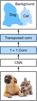
Here we describe the basic design of the fully convolutional network model. As shown in Figure 20.11.1, this model first uses a CNN to extract image features, then transforms the number of channels into the number of classes via a \(1\times 1\) convolutional layer, and finally transforms the height and width of the feature maps to those of the input image via the transposed convolution introduced in Section 20.10. As a result, the model output has the same height and width as the input image, where the output channel contains the predicted classes for the input pixel at the same spatial position.
Below, we use a ResNet model pretrained on the ImageNet dataset to extract image features and denote the model instance as pretrained_net. The last few layers of this model include a global average pooling layer and a fully connected layer: they are not needed in the fully convolutional network.
pretrained_net = torchvision.models.resnet18(
    weights=torchvision.models.ResNet18_Weights.DEFAULT)
list(pretrained_net.children())[-3:]
[Sequential(
(0): BasicBlock(
(conv1): Conv2d(256, 512, kernel_size=(3, 3), stride=(2, 2), padding=(1, 1), bias=False)
(bn1): BatchNorm2d(512, eps=1e-05, momentum=0.1, affine=True, track_running_stats=True)
(relu): ReLU(inplace=True)
(conv2): Conv2d(512, 512, kernel_size=(3, 3), stride=(1, 1), padding=(1, 1), bias=False)
(bn2): BatchNorm2d(512, eps=1e-05, momentum=0.1, affine=True, track_running_stats=True)
(downsample): Sequential(
(0): Conv2d(256, 512, kernel_size=(1, 1), stride=(2, 2), bias=False)
(1): BatchNorm2d(512, eps=1e-05, momentum=0.1, affine=True, track_running_stats=True)
)
)
(1): BasicBlock(
(conv1): Conv2d(512, 512, kernel_size=(3, 3), stride=(1, 1), padding=(1, 1), bias=False)
(bn1): BatchNorm2d(512, eps=1e-05, momentum=0.1, affine=True, track_running_stats=True)
(relu): ReLU(inplace=True)
(conv2): Conv2d(512, 512, kernel_size=(3, 3), stride=(1, 1), padding=(1, 1), bias=False)
(bn2): BatchNorm2d(512, eps=1e-05, momentum=0.1, affine=True, track_running_stats=True)
)
),
AdaptiveAvgPool2d(output_size=(1, 1)),
Linear(in_features=512, out_features=1000, bias=True)]# Note: keras.applications does not bundle a ResNet-18; it only ships
# ResNet-50/101/152. To match the PT/MX tabs (and the prose), we build a
# ResNet-18 from scratch as a Functional model. Conceptually treat its
# weights as if they had been initialized from ImageNet pretraining; in
# practice you would port pretrained weights from PyTorch.
def _resnet_block(x, num_channels, strides=1, use_1x1conv=False):
y = keras.layers.Conv2D(num_channels, 3, strides=strides,
padding='same', use_bias=False)(x)
y = keras.layers.BatchNormalization()(y)
y = keras.layers.ReLU()(y)
y = keras.layers.Conv2D(num_channels, 3, strides=1,
padding='same', use_bias=False)(y)
y = keras.layers.BatchNormalization()(y)
if use_1x1conv:
x = keras.layers.Conv2D(num_channels, 1, strides=strides,
use_bias=False)(x)
x = keras.layers.BatchNormalization()(x)
return keras.layers.ReLU()(y + x)
inputs = keras.Input(shape=(None, None, 3))
x = keras.layers.Conv2D(64, 7, strides=2, padding='same',
use_bias=False)(inputs)
x = keras.layers.BatchNormalization()(x)
x = keras.layers.ReLU()(x)
x = keras.layers.MaxPool2D(pool_size=3, strides=2, padding='same')(x)
x = _resnet_block(x, 64)
x = _resnet_block(x, 64)
x = _resnet_block(x, 128, strides=2, use_1x1conv=True)
x = _resnet_block(x, 128)
x = _resnet_block(x, 256, strides=2, use_1x1conv=True)
x = _resnet_block(x, 256)
x = _resnet_block(x, 512, strides=2, use_1x1conv=True)
features = _resnet_block(x, 512)
# Mirror the structure of torchvision.models.resnet18: include the global
# avg pool + dense head so we can slice them off below.
pooled = keras.layers.GlobalAveragePooling2D()(features)
logits = keras.layers.Dense(1000)(pooled)
pretrained_net = keras.Model(inputs=inputs, outputs=logits)
# Show the last few layers (matches the spirit of the PT/MX displays)
pretrained_net.layers[-3:][<ReLU name=re_lu_16, built=True>,
<GlobalAveragePooling2D name=global_average_pooling2d, built=True>,
<Dense name=dense, built=True>]pretrained_net = ResNet50.from_pretrained()
dummy = jnp.ones((1, 320, 480, 3))
print('Feature extractor output shape:',
pretrained_net.feature_map(dummy).shape)Feature extractor output shape: (1, 10, 15, 2048)pretrained_net = gluon.model_zoo.vision.resnet18_v2(pretrained=True)
pretrained_net.features[-3:], pretrained_net.output(HybridSequential(
(0): Activation(relu)
(1): GlobalAvgPool2D(size=(1, 1), stride=(1, 1), padding=(0, 0), ceil_mode=True, global_pool=True, pool_type=avg, layout=NCHW)
(2): Flatten
),
Dense(512 -> 1000, linear))Next, we create the fully convolutional network instance net. It copies all the pretrained convolutional layers in the ResNet except for the final global average pooling layer and the fully connected layer that are closest to the output.
net = nn.Sequential(*list(pretrained_net.children())[:-2])# Build the FCN feature extractor: all layers up to (but not including)
# the global average pooling and dense head — i.e., the full conv body.
# The last conv-block output (`features`) is the 1/32-resolution feature
# map; we use it as the new model output, dropping GAP + Dense.
net = keras.Model(inputs=pretrained_net.input, outputs=features)# `feature_map` omits the global average pooling and classification head.net = nn.HybridSequential()
for layer in pretrained_net.features[:-2]:
net.add(layer)Given an input with height and width of 320 and 480 respectively, the forward propagation of net reduces the input height and width to 1/32 of the original, namely 10 and 15.
X = torch.rand(size=(1, 3, 320, 480))
net(X).shape
torch.Size([1, 512, 10, 15])X = tf.random.uniform(shape=(1, 320, 480, 3))
net(X).shapeTensorShape([1, 10, 15, 512])X = jnp.ones((1, 320, 480, 3))
pretrained_net.feature_map(X).shape(1, 10, 15, 2048)X = np.random.uniform(size=(1, 3, 320, 480))
net(X).shape(1, 512, 10, 15)Next, we use a \(1\times 1\) convolutional layer to transform the number of output channels into the number of classes (21) of the Pascal VOC2012 dataset. Finally, we need to increase the height and width of the feature maps by 32 times to change them back to the height and width of the input image. Recall how to calculate the output shape of a convolutional layer in Section 6.3. Since \((320-64+16\times2+32)/32=10\) and \((480-64+16\times2+32)/32=15\), we construct a transposed convolutional layer with stride of \(32\), setting the height and width of the kernel to \(64\), the padding to \(16\). In general, we can see that for stride \(s\), padding \(s/2\) (assuming \(s/2\) is an integer), and the height and width of the kernel \(2s\), the transposed convolution will increase the height and width of the input by \(s\) times.
num_classes = 21
net.add_module('final_conv', nn.Conv2d(512, num_classes, kernel_size=1))
net.add_module('transpose_conv', nn.ConvTranspose2d(num_classes, num_classes,
                                    kernel_size=64, padding=16, stride=32))
num_classes = 21
# 1x1 conv to reduce channels to num_classes
final_conv = keras.layers.Conv2D(num_classes, kernel_size=1,
kernel_initializer='glorot_uniform')
# Transposed conv: stride=32, kernel=64, padding='same' upsamples 32x
# (for input height/width divisible by 32, output equals input spatial size)
transpose_conv = keras.layers.Conv2DTranspose(
num_classes, kernel_size=64, strides=32, padding='same', use_bias=False)
inputs = net.input
x = net.output
x = final_conv(x)
x = transpose_conv(x)
fcn_net = keras.Model(inputs=inputs, outputs=x)
print('FCN output shape:', fcn_net(tf.random.uniform((1, 320, 480, 3))).shape)FCN output shape: (1, 320, 480, 21)num_classes = 21
class FCN(nnx.Module):
"""Fully Convolutional Network for semantic segmentation."""
def __init__(self, backbone, num_classes, *, rngs):
self.backbone = backbone
self.classifier = nnx.Conv(2048, num_classes, (1, 1), rngs=rngs)
self.upsample = nnx.ConvTranspose(
num_classes, num_classes, (64, 64), strides=32, padding='SAME',
use_bias=False, rngs=rngs)
def __call__(self, X):
X = self.backbone.feature_map(X)
return self.upsample(self.classifier(X))
net = FCN(pretrained_net, num_classes, rngs=nnx.Rngs(0))
print('FCN output shape:',
net(jnp.ones((1, 320, 480, 3))).shape)FCN output shape: (1, 320, 480, 21)num_classes = 21
net.add(nn.Conv2D(num_classes, kernel_size=1),
nn.Conv2DTranspose(
num_classes, kernel_size=64, padding=16, strides=32))20.11.2 Initializing Transposed Convolutional Layers
We already know that transposed convolutional layers can increase the height and width of feature maps. In image processing, we may need to scale up an image, i.e., upsampling. Bilinear interpolation is one of the commonly used upsampling techniques. It is also often used for initializing transposed convolutional layers.
To explain bilinear interpolation, say that given an input image we want to calculate each pixel of the upsampled output image. In order to calculate the pixel of the output image at coordinate \((x, y)\), first map \((x, y)\) to coordinate \((x', y')\) on the input image, for example, according to the ratio of the input size to the output size. Note that the mapped \(x'\) and \(y'\) are real numbers. Then, find the four pixels closest to coordinate \((x', y')\) on the input image. Finally, the pixel of the output image at coordinate \((x, y)\) is calculated based on these four closest pixels on the input image and their relative distance from \((x', y')\).
Upsampling of bilinear interpolation can be implemented by the transposed convolutional layer with the kernel constructed by the following bilinear_kernel function. Due to space limitations, we only provide the implementation of the bilinear_kernel function below without discussions on its algorithm design.
def bilinear_kernel(in_channels, out_channels, kernel_size):
    factor = (kernel_size + 1) // 2
    if kernel_size % 2 == 1:
        center = factor - 1
    else:
        center = factor - 0.5
    og = (torch.arange(kernel_size).reshape(-1, 1),
          torch.arange(kernel_size).reshape(1, -1))
    filt = (1 - torch.abs(og[0] - center) / factor) * \
           (1 - torch.abs(og[1] - center) / factor)
    weight = torch.zeros((in_channels, out_channels,
                          kernel_size, kernel_size))
    weight[range(in_channels), range(out_channels), :, :] = filt
    return weight
def bilinear_kernel(in_channels, out_channels, kernel_size):
factor = (kernel_size + 1) // 2
if kernel_size % 2 == 1:
center = factor - 1
else:
center = factor - 0.5
og = (np.arange(kernel_size).reshape(-1, 1),
np.arange(kernel_size).reshape(1, -1))
filt = (1 - np.abs(og[0] - center) / factor) * \
(1 - np.abs(og[1] - center) / factor)
# Keras Conv2DTranspose uses HWIO kernel format (height, width, out, in)
weight = np.zeros((kernel_size, kernel_size, out_channels, in_channels),
dtype=np.float32)
for i in range(min(in_channels, out_channels)):
weight[:, :, i, i] = filt
return weightdef bilinear_kernel(in_channels, out_channels, kernel_size):
factor = (kernel_size + 1) // 2
if kernel_size % 2 == 1:
center = factor - 1
else:
center = factor - 0.5
og = (np.arange(kernel_size).reshape(-1, 1),
np.arange(kernel_size).reshape(1, -1))
filt = (1 - np.abs(og[0] - center) / factor) * \
(1 - np.abs(og[1] - center) / factor)
# Flax uses HWIO format for ConvTranspose kernels
weight = np.zeros((kernel_size, kernel_size, in_channels, out_channels))
for i in range(min(in_channels, out_channels)):
weight[:, :, i, i] = filt
return jnp.array(weight)def bilinear_kernel(in_channels, out_channels, kernel_size):
factor = (kernel_size + 1) // 2
if kernel_size % 2 == 1:
center = factor - 1
else:
center = factor - 0.5
og = (np.arange(kernel_size).reshape(-1, 1),
np.arange(kernel_size).reshape(1, -1))
filt = (1 - np.abs(og[0] - center) / factor) * \
(1 - np.abs(og[1] - center) / factor)
weight = np.zeros((in_channels, out_channels, kernel_size, kernel_size))
weight[range(in_channels), range(out_channels), :, :] = filt
return np.array(weight)Let’s experiment with upsampling of bilinear interpolation that is implemented by a transposed convolutional layer. We construct a transposed convolutional layer that doubles the height and weight, and initialize its kernel with the bilinear_kernel function.
conv_trans = nn.ConvTranspose2d(3, 3, kernel_size=4, padding=1, stride=2,
                                bias=False)
with torch.no_grad():
    conv_trans.weight.copy_(bilinear_kernel(3, 3, 4));
# Build a transposed conv layer with bilinear initialization to double H and W
bilinear_w = bilinear_kernel(3, 3, 4)
conv_trans = keras.layers.Conv2DTranspose(
3, kernel_size=4, strides=2, padding='same', use_bias=False,
kernel_initializer=tf.constant_initializer(bilinear_w))
# Build the layer by passing a dummy input
_ = conv_trans(tf.zeros((1, 1, 1, 3)))class BilinearConvTranspose(nnx.Module):
"""A transposed conv layer initialized with bilinear interpolation."""
def __init__(self, channels, kernel_size, strides, *, rngs):
self.layer = nnx.ConvTranspose(
channels, channels, (kernel_size, kernel_size), strides=strides,
padding='SAME', use_bias=False, rngs=rngs)
self.layer.kernel[...] = bilinear_kernel(
channels, channels, kernel_size)
def __call__(self, X):
return self.layer(X)
conv_trans = BilinearConvTranspose(3, 4, (2, 2), rngs=nnx.Rngs(0))conv_trans = nn.Conv2DTranspose(3, kernel_size=4, padding=1, strides=2)
conv_trans.initialize(init.Constant(bilinear_kernel(3, 3, 4)))Read the image X and assign the upsampling output to Y. In order to print the image, we need to adjust the position of the channel dimension.
img = torchvision.transforms.ToTensor()(d2l.Image.open('../img/catdog.jpg'))
X = img.unsqueeze(0)
Y = conv_trans(X)
out_img = Y[0].permute(1, 2, 0).detach()
img = np.array(Image.open('../img/catdog.jpg')).astype(np.float32) / 255
X = tf.expand_dims(tf.constant(img), axis=0) # NHWC
Y = conv_trans(X)
out_img = Y[0].numpy()img = np.array(Image.open('../img/catdog.jpg')).astype(np.float32) / 255
X = jnp.expand_dims(jnp.array(img), axis=0) # NHWC
Y = conv_trans(X)
out_img = np.array(Y[0])img = image.imread('../img/catdog.jpg')
X = np.expand_dims(img.astype('float32').transpose(2, 0, 1), axis=0) / 255
Y = conv_trans(X)
out_img = Y[0].transpose(1, 2, 0)As we can see, the transposed convolutional layer increases both the height and width of the image by a factor of two. Except for the different scales in coordinates, the image scaled up by bilinear interpolation and the original image printed in Section 20.3 look the same.
d2l.set_figsize()
print('input image shape:', img.permute(1, 2, 0).shape)
d2l.plt.imshow(img.permute(1, 2, 0));
print('output image shape:', out_img.shape)
d2l.plt.imshow(out_img);
input image shape: torch.Size([561, 728, 3])
output image shape: torch.Size([1122, 1456, 3])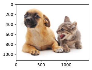
d2l.set_figsize()
print('input image shape:', img.shape)
d2l.plt.imshow(img);
print('output image shape:', out_img.shape)
d2l.plt.imshow(np.clip(out_img, 0, 1));
input image shape: (561, 728, 3)
output image shape: (1122, 1456, 3)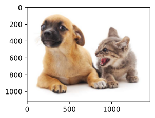
d2l.set_figsize()
print('input image shape:', img.shape)
d2l.plt.imshow(img);
print('output image shape:', out_img.shape)
d2l.plt.imshow(out_img);
input image shape: (561, 728, 3)
output image shape: (1122, 1456, 3)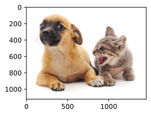
d2l.set_figsize()
print('input image shape:', img.shape)
d2l.plt.imshow(img.asnumpy());
print('output image shape:', out_img.shape)
d2l.plt.imshow(out_img.asnumpy());
input image shape: (561, 728, 3)
output image shape: (1122, 1456, 3)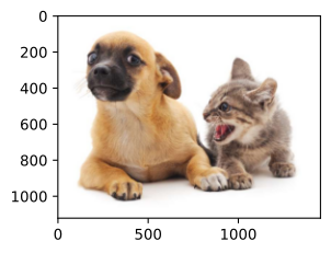
In a fully convolutional network, we initialize the transposed convolutional layer with upsampling of bilinear interpolation. For the \(1\times 1\) convolutional layer, we use Xavier initialization.
W = bilinear_kernel(num_classes, num_classes, 64)
net.transpose_conv.weight.data.copy_(W);
# Initialize the transpose conv kernel with bilinear upsampling weights.
# The 1x1 conv was already initialized with Glorot (Xavier) uniform above.
W = bilinear_kernel(num_classes, num_classes, 64)
# Find the Conv2DTranspose layer in fcn_net and set its weights
for layer in fcn_net.layers:
if isinstance(layer, keras.layers.Conv2DTranspose):
layer.set_weights([W])
break# Initialize the FCN with bilinear weights for the transposed conv layer
# and Xavier initialization for the 1x1 conv layer
W = bilinear_kernel(num_classes, num_classes, 64)
net.upsample.kernel[...] = WW = bilinear_kernel(num_classes, num_classes, 64)
net[-1].initialize(init.Constant(W))
net[-2].initialize(init=init.Xavier())20.11.3 Reading the Dataset
We read the semantic segmentation dataset as introduced in Section 20.9. The output image shape of random cropping is specified as \(320\times 480\): both the height and width are divisible by \(32\).
batch_size, crop_size = 32, (320, 480)
train_iter, test_iter = d2l.load_data_voc(batch_size, crop_size)
read 1114 examples
read 1078 examplesbatch_size, crop_size = 32, (320, 480)
train_iter, test_iter = d2l.load_data_voc(batch_size, crop_size)read 1114 examples
read 1078 examples# The NNX ResNet-50 is deeper than the ResNet-18 used in the PyTorch tab, so
# use a smaller minibatch while keeping the same crops and number of epochs.
batch_size, crop_size = 4, (320, 480)
train_iter, test_iter = d2l.load_data_voc(batch_size, crop_size)read 1114 examples
read 1078 examplesbatch_size, crop_size = 32, (320, 480)
train_iter, test_iter = d2l.load_data_voc(batch_size, crop_size)read 1114 examples
read 1078 examples20.11.4 Training
Now we can train our constructed fully convolutional network. The loss function and accuracy calculation here are not essentially different from those in image classification of earlier chapters. Because we use the output channel of the transposed convolutional layer to predict the class for each pixel, the channel dimension is specified in the loss calculation. In addition, the accuracy is calculated based on correctness of the predicted class for all the pixels.
def loss(inputs, targets):
    return F.cross_entropy(inputs, targets, reduction='none').mean(1).mean(1)

num_epochs, lr, wd, devices = 5, 0.001, 1e-3, d2l.try_all_gpus()
trainer = torch.optim.SGD(net.parameters(), lr=lr, weight_decay=wd)
d2l.train_ch13(net, train_iter, test_iter, loss, trainer, num_epochs, devices)
loss 0.411, train acc 0.870, test acc 0.851
351.0 examples/sec on [device(type='cuda', index=0)]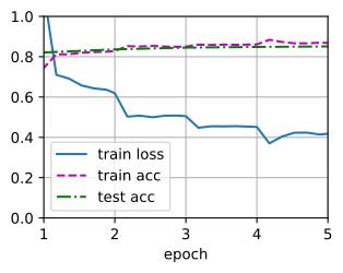
# Loss: SparseCategoricalCrossentropy over per-pixel logits (NHWC -> NHW).
# Full fine-tuning of the entire network (backbone + head) to match the
# PyTorch tab.
num_epochs, lr, wd = 5, 0.001, 1e-3
fcn_net.compile(
    optimizer=keras.optimizers.SGD(learning_rate=lr, weight_decay=wd),
    loss=keras.losses.SparseCategoricalCrossentropy(from_logits=True),
    metrics=['accuracy'],
    # Keras may otherwise select XLA automatically. For this unusually large
    # transposed convolution, XLA's cuDNN autotuning can take tens of minutes
    # before the first training step and offers no benefit to this example.
    jit_compile=False)
fcn_net.fit(train_iter, epochs=num_epochs, validation_data=test_iter,
            verbose=2)
Epoch 1/5
34/34 - 44s - 1s/step - accuracy: 0.3790 - loss: 2.5847 - val_accuracy: 0.7193 - val_loss: 2.6590
Epoch 2/5
34/34 - 10s - 297ms/step - accuracy: 0.7040 - loss: 1.5470 - val_accuracy: 0.7288 - val_loss: 2.0669
Epoch 3/5
34/34 - 9s - 274ms/step - accuracy: 0.7104 - loss: 1.4708 - val_accuracy: 0.7287 - val_loss: 1.6975
Epoch 4/5
34/34 - 9s - 279ms/step - accuracy: 0.7121 - loss: 1.4293 - val_accuracy: 0.7290 - val_loss: 1.5018
Epoch 5/5
34/34 - 10s - 280ms/step - accuracy: 0.7119 - loss: 1.4044 - val_accuracy: 0.7283 - val_loss: 1.4144<keras.src.callbacks.history.History at 0x74b1fc18f230>num_epochs, lr, wd = 5, 0.001, 1e-3
def parameter_labels(params):
return jax.tree_util.tree_map_with_path(
lambda path, _: ('head' if any(
getattr(p, 'key', None) in ('classifier', 'upsample')
for p in path) else 'backbone'), params)
optimizer = nnx.Optimizer(
net, optax.multi_transform(
{'head': optax.chain(optax.add_decayed_weights(wd),
optax.sgd(lr * 10)),
'backbone': optax.chain(optax.add_decayed_weights(wd),
optax.sgd(lr))},
parameter_labels),
wrt=nnx.Param)
eval_net = nnx.view(net, use_running_average=True, raise_if_not_found=False)
@nnx.jit
def train_step(model, optimizer, X, Y):
def loss_fn(model):
logits = model(X)
loss = optax.softmax_cross_entropy_with_integer_labels(logits, Y)
return loss.mean(), logits
(loss, logits), grads = nnx.value_and_grad(loss_fn, has_aux=True)(model)
optimizer.update(model, grads)
correct = (jnp.argmax(logits, axis=-1) == Y).sum()
return loss, correct
@nnx.jit
def eval_step(model, X, Y):
logits = model(X)
losses = optax.softmax_cross_entropy_with_integer_labels(logits, Y)
correct = (jnp.argmax(logits, axis=-1) == Y).sum()
return losses.sum(), correct
for epoch in range(num_epochs):
loss_terms, correct_terms, num_pixels = [], [], 0
for X, Y in train_iter:
X = jnp.transpose(jnp.array(X), (0, 2, 3, 1))
Y = jnp.array(Y)
loss, correct = train_step(net, optimizer, X, Y)
loss_terms.append(loss * Y.size)
correct_terms.append(correct)
num_pixels += Y.size
val_loss_terms, val_correct_terms, val_pixels = [], [], 0
for X, Y in test_iter:
X = jnp.transpose(jnp.array(X), (0, 2, 3, 1))
Y = jnp.array(Y)
val_loss, val_correct = eval_step(eval_net, X, Y)
val_loss_terms.append(val_loss)
val_correct_terms.append(val_correct)
val_pixels += Y.size
loss_sum = float(jnp.stack(loss_terms).sum())
correct = int(jnp.stack(correct_terms).sum())
val_loss_sum = float(jnp.stack(val_loss_terms).sum())
val_correct = int(jnp.stack(val_correct_terms).sum())
print(f'epoch {epoch + 1}, loss {loss_sum / num_pixels:.3f}, '
f'pixel acc {correct / num_pixels:.3f}, '
f'val loss {val_loss_sum / val_pixels:.3f}, '
f'val pixel acc {val_correct / val_pixels:.3f}')epoch 1, loss 1.621, pixel acc 0.706, val loss 1.201, val pixel acc 0.731
epoch 2, loss 1.143, pixel acc 0.737, val loss 1.091, val pixel acc 0.749
epoch 3, loss 1.030, pixel acc 0.755, val loss 0.971, val pixel acc 0.762
epoch 4, loss 0.940, pixel acc 0.772, val loss 0.905, val pixel acc 0.778
epoch 5, loss 0.866, pixel acc 0.787, val loss 0.836, val pixel acc 0.792num_epochs, lr, wd, devices = 5, 0.001, 1e-3, d2l.try_all_gpus()
loss = gluon.loss.SoftmaxCrossEntropyLoss(axis=1)
net.reset_ctx(devices)
trainer = gluon.Trainer(net.collect_params(), 'sgd',
{'learning_rate': lr, 'wd': wd})
d2l.train_ch13(net, train_iter, test_iter, loss, trainer, num_epochs, devices)loss 0.376, train acc 0.880, test acc 0.847
164.5 examples/sec on [gpu(0)]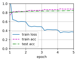
20.11.5 Prediction
When predicting, we need to standardize the input image in each channel and transform the image into the four-dimensional input format required by the CNN.
def predict(img):
    net.eval()
    X = test_iter.dataset.normalize_image(img).unsqueeze(0)
    with torch.no_grad():
        pred = net(X.to(devices[0])).argmax(dim=1)
    return pred.reshape(pred.shape[1], pred.shape[2])
def predict(img):
rgb_mean = np.array([0.485, 0.456, 0.406], dtype=np.float32)
rgb_std = np.array([0.229, 0.224, 0.225], dtype=np.float32)
X = (img.astype(np.float32) / 255 - rgb_mean) / rgb_std
X = tf.expand_dims(tf.constant(X), axis=0) # NHWC
pred = fcn_net(X, training=False) # (1, H, W, num_classes)
return tf.reshape(tf.argmax(pred, axis=-1), pred.shape[1:3])def predict(img):
rgb_mean = np.array([0.485, 0.456, 0.406])
rgb_std = np.array([0.229, 0.224, 0.225])
X = (img.astype(np.float32) / 255 - rgb_mean) / rgb_std
X = jnp.expand_dims(jnp.array(X), axis=0) # NHWC
pred = nnx.view(net, use_running_average=True,
raise_if_not_found=False)(X)
return jnp.argmax(pred, axis=-1).reshape(pred.shape[1], pred.shape[2])def predict(img):
X = test_iter._dataset.normalize_image(img)
X = np.expand_dims(X.transpose(2, 0, 1), axis=0)
pred = net(X.as_in_ctx(devices[0])).argmax(axis=1)
return pred.reshape(pred.shape[1], pred.shape[2])To visualize the predicted class of each pixel, we map the predicted class back to its label color in the dataset.
def label2image(pred):
    colormap = torch.tensor(d2l.VOC_COLORMAP, device=devices[0])
    X = pred.long()
    return colormap[X, :]
def label2image(pred):
colormap = tf.constant(d2l.VOC_COLORMAP, dtype=tf.uint8)
X = tf.cast(pred, tf.int32)
return tf.gather(colormap, X)def label2image(pred):
colormap = jnp.array(d2l.VOC_COLORMAP, dtype=jnp.uint8)
X = pred.astype(jnp.int32)
return colormap[X, :]def label2image(pred):
colormap = np.array(d2l.VOC_COLORMAP, ctx=devices[0], dtype='uint8')
X = pred.astype('int32')
return colormap[X, :]Images in the test dataset vary in size and shape. Since the model uses a transposed convolutional layer with stride of 32, when the height or width of an input image is indivisible by 32, the output height or width of the transposed convolutional layer will deviate from the shape of the input image. In order to address this issue, we can crop multiple rectangular areas with height and width that are integer multiples of 32 in the image, and perform forward propagation on the pixels in these areas separately. Note that the union of these rectangular areas needs to completely cover the input image. When a pixel is covered by multiple rectangular areas, the average of the transposed convolution outputs in separate areas for this same pixel can be input to the softmax operation to predict the class.
For simplicity, we only read a few larger test images, and crop a \(320\times480\) area for prediction starting from the upper-left corner of an image. For these test images, we print their cropped areas, prediction results, and ground-truth row by row.
voc_dir = d2l.download_extract('voc2012', 'VOCdevkit/VOC2012')
test_images, test_labels = d2l.read_voc_images(voc_dir, False)
n, imgs = 4, []
for i in range(n):
    crop_rect = (0, 0, 320, 480)
    X = torchvision.transforms.functional.crop(test_images[i], *crop_rect)
    pred = label2image(predict(X))
    imgs += [X.permute(1,2,0), pred.cpu(),
             torchvision.transforms.functional.crop(
                 test_labels[i], *crop_rect).permute(1,2,0)]
d2l.show_images(imgs[::3] + imgs[1::3] + imgs[2::3], 3, n, scale=2);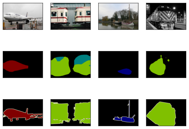
voc_dir = d2l.download_extract('voc2012', 'VOCdevkit/VOC2012')
test_images, test_labels = d2l.read_voc_images(voc_dir, False)
n, imgs = 4, []
for i in range(n):
    # Crop HWC arrays: top=0, left=0, height=320, width=480
    X = test_images[i][:320, :480, :]
    pred = label2image(predict(X))
    label_crop = test_labels[i][:320, :480, :]
    imgs += [X, pred.numpy(), label_crop]
d2l.show_images(imgs[::3] + imgs[1::3] + imgs[2::3], 3, n, scale=2);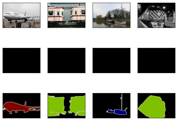
voc_dir = d2l.download_extract('voc2012', 'VOCdevkit/VOC2012')
test_images, test_labels = d2l.read_voc_images(voc_dir, False)
n, imgs = 4, []
for i in range(n):
    # Crop HWC arrays: top=0, left=0, height=320, width=480
    X = test_images[i][:320, :480, :]
    pred = label2image(predict(X))
    label_crop = test_labels[i][:320, :480, :]
    imgs += [X, np.array(pred), label_crop]
d2l.show_images(imgs[::3] + imgs[1::3] + imgs[2::3], 3, n, scale=2);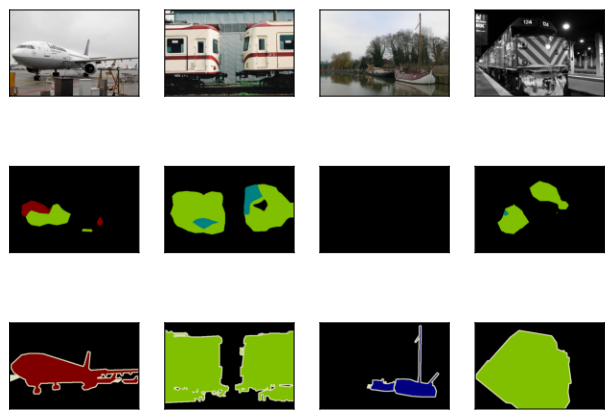
voc_dir = d2l.download_extract('voc2012', 'VOCdevkit/VOC2012')
test_images, test_labels = d2l.read_voc_images(voc_dir, False)
n, imgs = 4, []
for i in range(n):
    crop_rect = (0, 0, 480, 320)
    X = image.fixed_crop(test_images[i], *crop_rect)
    pred = label2image(predict(X))
    imgs += [X, pred, image.fixed_crop(test_labels[i], *crop_rect)]
d2l.show_images(imgs[::3] + imgs[1::3] + imgs[2::3], 3, n, scale=2);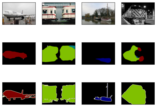
20.11.6 Summary
- The fully convolutional network first uses a CNN to extract image features, then transforms the number of channels into the number of classes via a \(1\times 1\) convolutional layer, and finally transforms the height and width of the feature maps to those of the input image via the transposed convolution.
- In a fully convolutional network, we can use upsampling of bilinear interpolation to initialize the transposed convolutional layer.
20.11.7 Exercises
- If we use Xavier initialization for the transposed convolutional layer in the experiment, how does the result change?
- Can you further improve the accuracy of the model by tuning the hyperparameters?
- Predict the classes of all pixels in test images.
- The original fully convolutional network paper also uses outputs of some intermediate CNN layers (Long et al. 2015). Try to implement this idea.