from scipy import optimize
from scipy.stats import norm37.4 Test Functions and Transport
A model whose samples miss the data learns nothing from an f-divergence. On disjoint supports every member of that family is a constant (Section 37.3.1.2), and a constant has no gradient. The verdict rested on two point masses, the extreme case. Real distributions have spread: two Gaussians overlap everywhere, because their tails never reach zero. Does a little overlap bring the gradient back? The f-divergences left a second complaint as well. They need the ratio \(p/q\), which samples do not supply, so a critic had to be trained before anything could be measured (Section 37.3.4). Can two samples be compared with no critic at all?
We can settle the first question with numbers. Let the data be \(P = \mathcal{N}(0, 1)\) and the model \(Q = \mathcal{N}(d, 1)\), the same bell curve \(d\) standard deviations away, with \(d\) the model’s one parameter. After the imports, a cell evaluates the five comparisons of Table 37.3.1 on this pair, each with its slope in \(d\), the gradient that the model receives. Its formulas are derived in this section and the last; for now, read only the output, which we shall call the opening table.
def js(d, x=np.linspace(-12, 20, 6401)):
    """JS divergence of N(0, 1) and N(d, 1) by quadrature on the grid x."""
    log_p, log_q = norm.logpdf(x), norm.logpdf(x, loc=d)
    log_m = np.logaddexp(log_p, log_q) - math.log(2)    # log of the mixture
    terms = np.exp(log_p) * (log_p - log_m) + np.exp(log_q) * (log_q - log_m)
    return terms.sum() * (x[1] - x[0]) / 2

comparisons = {                       # N(0, 1) against N(d, 1), RBF ell = 1
    'KL': lambda d: d ** 2 / 2,
    'JS': js,
    'TV': lambda d: 2 * norm.cdf(d / 2) - 1,
    'MMD^2': lambda d: 2 / math.sqrt(3) * (1 - math.exp(-d ** 2 / 6)),
    'W1': lambda d: d}
h = 1e-3                              # step of the central difference
print('   d' + ''.join(f'{name:>8s} {"slope":>7s}' for name in comparisons))
for d in (0.5, 1.0, 2.0, 4.0, 8.0):
    print(f'{d:4.1f}' + ''.join(
        f'{f(d):8.3f} {(f(d + h) - f(d - h)) / (2 * h):7.1e}'
        for f in comparisons.values()))
d KL slope JS slope TV slope MMD^2 slope W1 slope
0.5 0.125 5.0e-01 0.030 1.2e-01 0.197 3.9e-01 0.047 1.8e-01 0.500 1.0e+00
1.0 0.500 1.0e+00 0.111 2.0e-01 0.383 3.5e-01 0.177 3.3e-01 1.000 1.0e+00
2.0 2.000 2.0e+00 0.337 2.2e-01 0.683 2.4e-01 0.562 4.0e-01 2.000 1.0e+00
4.0 8.000 4.0e+00 0.633 6.9e-02 0.954 5.4e-02 1.074 1.1e-01 4.000 1.0e+00
8.0 32.000 8.0e+00 0.693 2.0e-04 1.000 1.3e-04 1.155 7.2e-05 8.000 1.0e+00At half a standard deviation all five slopes lie between \(0.1\) and \(1\), and any of the comparisons would train the model. At \(d = 8\) the Jensen–Shannon divergence reads \(0.693\) and total variation \(1.000\), the constants \(\log 2\) and \(1\) of the point masses, and both slopes are near \(10^{-4}\). Overlap in the tails does not help. The KL divergence keeps a slope, \(d\) itself, but only because a Gaussian model has a density at every data point; a model whose samples lie on a thin surface has none. That leaves the two comparisons that kept moving for the point masses. \(\textrm{MMD}^2\) grows at first and has stalled by \(d = 8\), at \(1.155\) with a slope below \(10^{-4}\). \(W_1\) equals \(d\), with slope \(1\) at every distance.
Neither is built from the ratio \(p/q\). MMD compares how \(P\) and \(Q\) average a class of functions; samples can estimate averages, and the class decides how far the comparison sees. \(W_1\) asks how far mass must travel to turn one distribution into the other, and it turns out to be a comparison of averages too. Two results stand out. Over a fixed set of features the comparison of averages has a closed form, with no second network to train. And the cost of moving mass equals the largest gap in averages over functions of slope at most one, the theorem behind the Wasserstein GAN of Section 16.2. \(P\) is the data and \(Q\) the model, as before, and the examples are on the line.
37.4.1 Integral Probability Metrics and MMD
37.4.1.1 Classes of Test Functions
Total variation is a metric, and still it went flat in the opening table. Its second form shows why, and what to change: total variation is the largest disagreement between \(P\) and \(Q\) about the probability of any event \(A\) (Section 37.3.3), \(\textrm{TV}(P, Q) = \sup_A |P(A) - Q(A)|\). The probability of an event is the average of its indicator function, so total variation is a supremum, over a class of functions, of the difference between two averages. Nothing obliges us to use indicators. For a class \(\mathcal{G}\) of test functions \(g\), the integral probability metric (IPM) (Müller 1997) is
\[ \textrm{IPM}_{\mathcal{G}}(P, Q) = \sup_{g \in \mathcal{G}} \,\big( \mathbb{E}_{x \sim P}[g(x)] - \mathbb{E}_{x \sim Q}[g(x)] \big). \tag{37.4.1}\]
The class \(\mathcal{G}\) is a panel of auditors, and the IPM reports the largest gap in averages that any auditor in the panel can find. Our classes contain \(-g\) along with every \(g\), so the gap is never negative and is the same in both directions; whether it vanishes only for \(P = Q\), as the word metric promises, depends on the class. The critic of Section 37.3.4 was an auditor too. In its bound, \(D_f(P\|Q) \geq \mathbb{E}_P[T] - \mathbb{E}_Q[f^*(T)]\) for every function \(T\), the conjugate \(f^*\) keeps an unrestricted critic in check. An IPM averages \(g\) itself under both distributions, so nothing restrains \(g\) except membership in \(\mathcal{G}\), and everything depends on the class.
Three classes matter to us. Functions with \(|g| \leq \tfrac{1}{2}\) give total variation again: an indicator minus \(\tfrac12\) is such a function, the constant cancels in the difference, and \(g = \tfrac12\,\textrm{sign}(p - q)\) attains the supremum. Functions that are linear in a fixed set of features give the maximum mean discrepancy (MMD) (Gretton et al. 2012), which we build next. Functions of slope at most one give the Wasserstein distance of Section 37.4.2.
Why not take the largest class every time? A class has to meet two requirements, and size works against the first: averages over a sample must track averages over the distribution. Samples estimate expectations directly, with no density ratio, but a panel that is too large finds gaps that are not there. Two samples of \(1{,}000\) points from the same continuous distribution share no point, so the indicator of the first sample has mean \(1\) on it and \(0\) on the other: the empirical total variation is \(1\) whatever the distributions are. A class must be small or smooth enough to exclude such functions.
The second requirement is that the gap keep growing as the distributions move apart, and for that the class needs functions that grow. Total variation has none: its test functions are bounded, so its gap cannot exceed \(1\). The largest disagreement is about the event \(\{p > q\}\), which for the two Gaussians of the opening is the half-line \(x < d/2\). Its two probabilities give \(\textrm{TV} = \Phi(d/2) - \Phi(-d/2) = 2\Phi(d/2) - 1\), where \(\Phi\) is the cumulative distribution function (CDF) of the standard normal. This is \(0.954\) at \(d = 4\) and within \(10^{-4}\) of \(1\) at \(d = 8\). Once an indicator separates the two bell curves almost perfectly, moving them further apart changes nothing. Total variation fails both requirements, and we shall hold the next two classes to them.
37.4.1.2 Mean Features and Kernels
We build a better class from the smallest panel up, and try each stage on one pair: \(\mathcal{N}(0, 1)\) against \(\mathcal{N}(0, 4)\), which differ in spread and not in mean. First, take linear test functions \(g(x) = w\, x\) with \(|w| \leq 1\). Then \(\mathbb{E}_P g - \mathbb{E}_Q g = w\,(\mathbb{E}_P X - \mathbb{E}_Q X)\), and the supremum is \(|\mathbb{E}_P X - \mathbb{E}_Q X|\): the IPM over linear functions is the difference of the means. It cannot see a change of spread, and on our pair it reports \(0\).
Second, add a feature. Take the feature vector \(\boldsymbol{\varphi}(x) = (x, x^2)\) and the test functions \(g(x) = \mathbf{w}^\top \boldsymbol{\varphi}(x)\) with \(\|\mathbf{w}\| \leq 1\), and write \(\mathbf{m}_P = \mathbb{E}_P[\boldsymbol{\varphi}(x)]\) for the mean feature of \(P\). Then \(\mathbb{E}_P g - \mathbb{E}_Q g = \mathbf{w}^\top(\mathbf{m}_P - \mathbf{m}_Q)\), and by the Cauchy–Schwarz inequality the largest value of a linear function on the unit ball is the norm of its coefficient vector:
\[ \textrm{MMD}(P, Q) = \sup_{\|\mathbf{w}\| \leq 1} \mathbf{w}^\top(\mathbf{m}_P - \mathbf{m}_Q) = \|\mathbf{m}_P - \mathbf{m}_Q\|. \tag{37.4.2}\]
MMD is the distance between the mean features, and the supremum has gone. On our pair the mean features are \((0, 1)\) and \((0, 4)\), so \(\textrm{MMD}^2 = 0^2 + 3^2 = 9\): means and second moments are now both compared.
Third, we expand the squared norm. A product of two means is the mean of a product over independent draws, so \(\|\mathbf{m}_P\|^2 = \mathbb{E}\langle\boldsymbol{\varphi}(x), \boldsymbol{\varphi}(x')\rangle\) for independent \(x, x'\) from \(P\). With independent \(y, y'\) from \(Q\) as well, \(\|\mathbf{m}_P - \mathbf{m}_Q\|^2 = \mathbb{E}\langle\boldsymbol{\varphi}(x), \boldsymbol{\varphi}(x')\rangle + \mathbb{E}\langle\boldsymbol{\varphi}(y), \boldsymbol{\varphi}(y')\rangle - 2\,\mathbb{E}\langle\boldsymbol{\varphi}(x), \boldsymbol{\varphi}(y)\rangle\). Only inner products of features appear. We call \(k(x, x') = \langle \boldsymbol{\varphi}(x), \boldsymbol{\varphi}(x')\rangle\) the kernel and obtain
\[ \textrm{MMD}^2(P, Q) = \mathbb{E}_{x, x' \sim P}[k(x, x')] + \mathbb{E}_{y, y' \sim Q}[k(y, y')] - 2\, \mathbb{E}_{x \sim P, y \sim Q}[k(x, y)]. \tag{37.4.3}\]
The first two terms measure similarity within each distribution and the third similarity across the two. If draws from \(P\) and \(Q\) interleave, the three terms cancel; if they form separate clumps, the within terms exceed the across term. The features of the first step have the linear kernel \(k(x, x') = x x'\), and those of the second the quadratic kernel \(x x' + x^2 x'^2\).
The quadratic kernel still has a blind spot: two distributions with equal means and equal variances are at distance zero. We could add \(x^3\), then \(x^4\), and never finish. The fourth step therefore chooses the kernel directly, as a measure of similarity, and never writes the features down. The RBF kernel \(k(x, x') = e^{-(x - x')^2/(2\ell^2)}\) calls two points similar when they lie within about a length scale \(\ell\) of each other. It is an inner product of features all the same. It factors as \(e^{-x^2/(2\ell^2)}\, e^{-x'^2/(2\ell^2)}\, e^{x x'/\ell^2}\), and the power series of the last factor writes it as an inner product of infinitely many features \(\varphi_j(x) = x^j e^{-x^2/(2\ell^2)} / (\ell^j \sqrt{j!})\), \(j = 0, 1, 2, \ldots\), damped monomials of every order with weights that decrease quickly. The panel now has infinitely many auditors, and its verdict is still three averages. In \(\mathbb{R}^n\) the squared difference in the kernel becomes a squared norm and nothing else changes.
No blind spot is left. With the RBF kernel, \(\textrm{MMD}(P, Q) = 0\) only if \(P = Q\) (Gretton et al. 2012), so this MMD is a metric. A kernel with this property is called characteristic; the linear and quadratic kernels are not.
For Gaussians the RBF averages can be computed by hand. For \(Z \sim \mathcal{N}(\mu, s^2)\), a Gaussian integral gives
\[ \mathbb{E}\big[e^{-Z^2/(2\ell^2)}\big] = \Big(1 + \frac{s^2}{\ell^2}\Big)^{-1/2} \exp\!\Big(-\frac{\mu^2}{2(\ell^2 + s^2)}\Big), \tag{37.4.4}\]
and the difference of two independent Gaussians is Gaussian with the variances added. On our pair at \(\ell = 1\) the three differences \(x - x'\), \(y - y'\) and \(x - y\) have mean zero and variances \(2\), \(8\) and \(5\), so \(\textrm{MMD}^2 = 3^{-1/2} + 9^{-1/2} - 2 \cdot 6^{-1/2} \approx 0.094\). For the two Gaussians of the opening the same integral gives \(\tfrac{2}{\sqrt{3}}\big(1 - e^{-d^2/6}\big)\), the \(\textrm{MMD}^2\) column of the opening table (Exercise 1a). For the point masses of Table 37.3.1 there is nothing to average, and Equation 37.4.3 gives \(1 + 1 - 2k(0, d) = 2 - 2e^{-d^2/2}\), the fourth row of that table. In both formulas only the cross term depends on \(d\), and it is gone within a few length scales. The gap stops growing, and the second requirement is not met. An RBF auditor is smooth, and it is nearsighted.
37.4.1.3 Estimation from Samples
The first requirement is where a kernel does well. From samples, each expectation in Equation 37.4.3 becomes an average over pairs. The unbiased estimator (Gretton et al. 2012) leaves out the pairs of a point with itself, which would bias the within terms upward. We apply it to \(N = 1{,}000\) draws from \(\mathcal{N}(0, 1)\) and as many from \(\mathcal{N}(0, 4)\) under the linear, quadratic and RBF kernels, for which we have just found \(0\), \(9\) and \(0.094\). With the RBF kernel we also compare the first sample with a second one from \(\mathcal{N}(0, 1)\), where the answer is \(0\), and with one from \(\mathcal{N}(0.5, 1)\), where the opening table says \(0.047\). What the mathematics does not supply is the size of the sampling error.
def mmd2_unbiased(x, y, k):
    """Unbiased MMD^2 between samples x and y for the kernel k(a, b)."""
    kxx = k(x[:, None], x[None, :])
    kyy = k(y[:, None], y[None, :])
    n, m = len(x), len(y)
    return ((kxx.sum() - np.trace(kxx)) / (n * (n - 1))
            + (kyy.sum() - np.trace(kyy)) / (m * (m - 1))
            - 2 * k(x[:, None], y[None, :]).mean())

linear = lambda a, b: a * b                         # features phi(x) = x
quadratic = lambda a, b: a * b + a ** 2 * b ** 2    # features (x, x^2)
rbf = lambda a, b: np.exp(-(a - b) ** 2 / 2)        # RBF kernel, ell = 1

rng = np.random.default_rng()
n = 1000
x_p = rng.standard_normal(n)                # P = N(0, 1)
y_var = 2 * rng.standard_normal(n)          # N(0, 4)
y_same = rng.standard_normal(n)             # N(0, 1) again
y_shift = rng.standard_normal(n) + 0.5      # N(0.5, 1)
for name, y, k, pop in [
        ('linear,    N(0,1) vs N(0,4)', y_var, linear, 0.0),
        ('quadratic, N(0,1) vs N(0,4)', y_var, quadratic, 9.0),
        ('RBF,       N(0,1) vs N(0,4)', y_var, rbf,
         3 ** -0.5 + 9 ** -0.5 - 2 * 6 ** -0.5),
        ('RBF,       N(0,1) vs N(0,1)', y_same, rbf, 0.0),
        ('RBF,       N(0,1) vs N(0.5,1)', y_shift, rbf,
         2 / np.sqrt(3) * (1 - np.exp(-1 / 24)))]:
    print(f'{name:30s} MMD^2 = {mmd2_unbiased(x_p, y, k):+.4f}  '
f'(population {pop:.4f})')linear, N(0,1) vs N(0,4) MMD^2 = -0.0033 (population 0.0000)
quadratic, N(0,1) vs N(0,4) MMD^2 = +10.2618 (population 9.0000)
RBF, N(0,1) vs N(0,4) MMD^2 = +0.1180 (population 0.0942)
RBF, N(0,1) vs N(0,1) MMD^2 = +0.0001 (population 0.0000)
RBF, N(0,1) vs N(0.5,1) MMD^2 = +0.0351 (population 0.0471)linear, N(0,1) vs N(0,4) MMD^2 = -0.0026 (population 0.0000)
quadratic, N(0,1) vs N(0,4) MMD^2 = +8.0798 (population 9.0000)
RBF, N(0,1) vs N(0,4) MMD^2 = +0.0971 (population 0.0942)
RBF, N(0,1) vs N(0,1) MMD^2 = +0.0025 (population 0.0000)
RBF, N(0,1) vs N(0.5,1) MMD^2 = +0.0534 (population 0.0471)linear, N(0,1) vs N(0,4) MMD^2 = +0.0142 (population 0.0000)
quadratic, N(0,1) vs N(0,4) MMD^2 = +8.3040 (population 9.0000)
RBF, N(0,1) vs N(0,4) MMD^2 = +0.0873 (population 0.0942)
RBF, N(0,1) vs N(0,1) MMD^2 = -0.0004 (population 0.0000)
RBF, N(0,1) vs N(0.5,1) MMD^2 = +0.0546 (population 0.0471)linear, N(0,1) vs N(0,4) MMD^2 = -0.0029 (population 0.0000)
quadratic, N(0,1) vs N(0,4) MMD^2 = +7.8546 (population 9.0000)
RBF, N(0,1) vs N(0,4) MMD^2 = +0.0929 (population 0.0942)
RBF, N(0,1) vs N(0,1) MMD^2 = +0.0010 (population 0.0000)
RBF, N(0,1) vs N(0.5,1) MMD^2 = +0.0501 (population 0.0471)The linear kernel reports a value near zero because the means agree. Its estimate is the squared difference of the two sample means, less an estimate of the variance of that difference, about \((1 + 4)/1{,}000 = 0.005\). It therefore cannot fall much below \(-0.005\), while about one run in twenty exceeds \(+0.015\). The quadratic kernel reports about \(9\), give or take \(3\); its estimate involves fourth powers and is noisy. The RBF kernel reports about \(0.094\), give or take \(0.03\), and for the shifted pair about \(0.047\), typically within \(0.02\), an error that can reach a third of the value. Between the two samples of \(\mathcal{N}(0, 1)\) the RBF estimate is far steadier, within a few thousandths of zero and sometimes below it, because the errors of the three averages then cancel to first order. Where the indicators found a gap of \(1\) between two samples of one distribution, the kernel finds none.
The RBF estimator measures the size of a difference poorly and detects its presence well, and this makes it a two-sample test: from \(1{,}000\) points, a value of a few hundredths is strong evidence that the samples differ in distribution. No critic was trained and no density was evaluated.
37.4.1.4 The Witness
An IPM is a supremum, so one may ask which auditor found the gap. For MMD the supremum in Equation 37.4.2 is attained by \(\mathbf{w}^\star \propto \mathbf{m}_P - \mathbf{m}_Q\), and the corresponding test function, the witness, \(g^\star(x) \propto \langle \mathbf{m}_P - \mathbf{m}_Q, \boldsymbol{\varphi}(x)\rangle = \mathbb{E}_P[k(x, X)] - \mathbb{E}_Q[k(x, Y)]\), needs only kernel evaluations. For the shifted pair, \(\mathcal{N}(0, 1)\) against \(\mathcal{N}(0.5, 1)\), the two densities are mirror images about \(x = 0.25\), so the witness of the two distributions changes sign there. We estimate the witness by sample means on a grid and plot it with the two densities. The cell also prints \(\mathbb{E}_P g - \mathbb{E}_Q g\) for the unscaled witness \(g = \langle \mathbf{m}_P - \mathbf{m}_Q, \boldsymbol{\varphi}\rangle\). This gap is \(\|\mathbf{m}_P - \mathbf{m}_Q\|^2\), which is \(\textrm{MMD}^2\) once more, estimated this time with the self-pairs included.
g = lambda s: (rbf(s[:, None], x_p[None, :]).mean(axis=1)    # the unscaled
               - rbf(s[:, None], y_shift[None, :]).mean(axis=1))  # witness
grid = np.linspace(-4.0, 4.5, 400)
witness = g(grid)
print(f'witness changes sign at x = {grid[np.argmax(witness < 0)]:.2f}')
print(f'E_P g - E_Q g = {g(x_p).mean() - g(y_shift).mean():.4f}')
d2l.plot(grid, [witness / np.abs(witness).max(), norm.pdf(grid),
                norm.pdf(grid, loc=0.5)], 'x', '',
         legend=['witness (scaled)', 'p = N(0, 1)', 'q = N(0.5, 1)'],
figsize=(5, 3))witness changes sign at x = 0.35
E_P g - E_Q g = 0.0360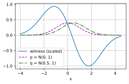
witness changes sign at x = 0.24
E_P g - E_Q g = 0.0542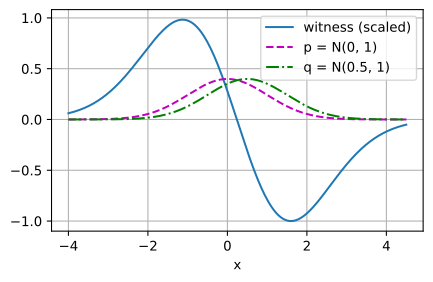
witness changes sign at x = 0.22
E_P g - E_Q g = 0.0554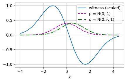
witness changes sign at x = 0.35
E_P g - E_Q g = 0.0509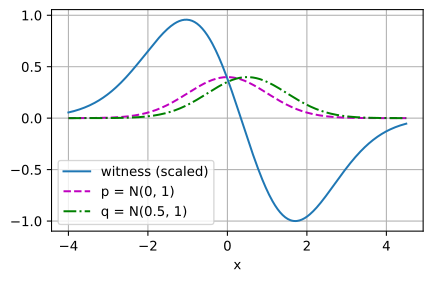
The witness is positive where \(P\) has more mass and negative where \(Q\) has more. It changes sign near \(x = 0.25\); with \(1{,}000\) points per sample the crossing moves by a tenth or two from draw to draw. The printed gap agrees with the last line of the previous output, the unbiased estimate for the same two samples, to about \(0.001\), and the difference is the self-pairs.
The ends of the plot say more than the crossing. A model that lowers the gap moves each of its samples uphill on the test function, so the slope of the test function at a sample is the push which that sample receives. The witness is steep between the two bell curves, and a few length scales away it levels off toward zero. A model sample out there is told nothing. This is the \(\textrm{MMD}^2\) column of the opening table, seen from one sample.
MMD with a fixed kernel therefore serves twice: as a two-sample test, and as a loss on which a model is trained without an adversary (Li et al. 2015). The kernel inception distance by which generated images are scored is the unbiased estimate of the previous subsection, applied to image features with a cubic kernel (Section 16.5). The length scale has to be chosen, and a poor choice is costly: at \(\ell = 1\) the slope at \(d = 8\) was \(7 \times 10^{-5}\) (Exercise 1b tries longer scales). Common practice sets \(\ell\) to the median distance between sample points, or adds RBF kernels of several length scales, as Section 16.2 does when it trains the model of a GAN, its generator, on MMD.
37.4.2 Optimal Transport and the Wasserstein Distance
One column of the opening table never went flat. \(W_1\) kept its slope because it measures distance itself, which the f-divergences ignore and a kernel sees only nearby: \(\delta_{0.01}\) is near \(\delta_0\) because its mass need only move \(0.01\). The idea is old. In 1781 Gaspard Monge asked how a heap of soil can be moved into a pit of the same volume with the least work, and the least work is a measure of how far the heap is from the pit.
37.4.2.1 Transport Plans
Take two distributions on the points \(0, 1, \ldots, 5\) of the line, with \(P\) mostly on the left and \(Q\) mostly on the right, as in the top left panel of Figure 37.4.1. To turn \(P\) into \(Q\) we must say how much mass travels from each source \(x\) to each destination \(y\). Such a transport plan is a joint distribution \(\gamma\) of pairs \((x, y)\) whose marginals are \(P\) and \(Q\): what leaves each \(x\) is what \(P\) has there, and what arrives at each \(y\) is what \(Q\) needs. A plan is also called a coupling of \(P\) and \(Q\). The Wasserstein-1 distance, also called the earth mover’s distance, is the least total of mass times distance over all plans. Writing \(\Pi(P, Q)\) for the set of plans, for \(P\) and \(Q\) on \(\mathbb{R}^n\) with finite first moments,
\[ W_1(P, Q) = \inf_{\gamma \in \Pi(P, Q)} \mathbb{E}_{(x, y) \sim \gamma}\big[ \|x - y\| \big]. \tag{37.4.5}\]
The \(1\) in the name is the power of the distance; the second power comes later. Between the point masses \(\delta_0\) and \(\delta_d\) the only plan moves all mass from \(0\) to \(d\), so \(W_1(\delta_0, \delta_d) = |d|\), with gradient \(\pm 1\) for \(d \neq 0\). For the two Gaussians of the opening, shifting every point by \(d\) is a plan of cost \(d\), and none is cheaper, because \(\mathbb{E}_\gamma|x - y| \geq |\mathbb{E}_\gamma[x - y]| = d\) for every plan. In both cases \(W_1\) is the distance itself, the training signal that the f-divergences lack.

37.4.2.2 Kantorovich–Rubinstein Duality
As a recipe for computation the definition is discouraging: it optimizes over joint distributions, which are hard even to parameterize from samples. On finitely many points it is at least a familiar kind of problem, a linear program. The unknowns are the entries of the plan, and the cost and the constraints on the marginals are linear in them. A linear program has a dual, a maximization over multipliers for its constraints (Section 35.7.1). The dual of transport optimizes over a single function, and it is the reason \(W_1\) matters to deep learning.
Proposition (Kantorovich–Rubinstein duality). For distributions \(P\) and \(Q\) on \(\mathbb{R}^n\) with finite first moments,
\[ W_1(P, Q) = \sup_{\|g\|_{\textrm{Lip}} \leq 1} \big( \mathbb{E}_{x \sim P}[g(x)] - \mathbb{E}_{y \sim Q}[g(y)] \big), \tag{37.4.6}\]
where the supremum runs over all 1-Lipschitz functions \(g\), those with \(|g(x) - g(y)| \leq \|x - y\|\) for all \(x, y\).
An infimum over plans has become a supremum over one function: \(W_1\) is the IPM Equation 37.4.1 over test functions of slope at most \(1\), the third of our classes. Such an auditor cannot jump, so it cannot pick out the points of a sample as an indicator does. It can climb without limit, however, and that is what the second requirement asked for. For the two Gaussians of the opening take \(g(x) = -x\). Its averages are \(0\) under \(P\) and \(-d\) under \(Q\), a gap of \(d\), which is \(W_1\), so no auditor of slope one does better. Its slope is the same at every model sample, however far from the data the sample lies, and uphill on \(g\) is the way to the data.
A network can represent such a function, and the WGAN (Arjovsky et al. 2017) trains this dual, with a neural critic in the role of \(g\) that is constrained to be approximately 1-Lipschitz. Section 16.2 sets this critic beside the other adversarial losses, and Section 16.4 treats the gradient penalties that enforce the constraint. What an approximately Lipschitz critic reports is, of course, no longer exactly \(W_1\).
37.4.2.3 Transport on the Line
We prove the duality only on the line, where the proof also yields a closed form and transport needs no optimization at all; Peyré and Cuturi (2019) give the general proof. The idea is to count crossings. At a point \(t\), \(P\) has a fraction \(F_P(t)\) of its mass at or to the left of \(t\) and \(Q\) has \(F_Q(t)\), so any plan must carry at least \(|F_P(t) - F_Q(t)|\) of mass across \(t\). A parcel moved from \(x\) to \(y\) crosses every \(t\) between them, so its distance \(|x - y|\) is the length of the set of points it crosses, and the total cost is the mass crossing each \(t\), integrated over \(t\).
Proposition (\(W_1\) on the line). For distributions \(P\) and \(Q\) on \(\mathbb{R}\) with CDFs \(F_P\), \(F_Q\) and finite first moments,
\[ W_1(P, Q) = \int_{-\infty}^{\infty} \lvert F_P(t) - F_Q(t) \rvert \, dt = \sup_{\|g\|_{\textrm{Lip}} \leq 1} \big( \mathbb{E}_P[g] - \mathbb{E}_Q[g] \big), \tag{37.4.7}\]
so Kantorovich–Rubinstein duality holds on the line.
Proof. Step 1: every plan costs at least the area. For \((X, Y) \sim \gamma\), \(|X - Y| = \int \mathbf{1}(t \textrm{ lies between } X \textrm{ and } Y)\, dt\). The integrand is non-negative, so expectation and integral may be exchanged:
\[ \mathbb{E}_\gamma|X - Y| = \int \Big( \gamma(X \leq t < Y) + \gamma(Y \leq t < X) \Big)\, dt \geq \int \big| \gamma(X \leq t < Y) - \gamma(Y \leq t < X) \big|\, dt. \]
The step that is not routine is the difference inside the last integral. Add and subtract \(\gamma(X \leq t, Y \leq t)\): then \(\gamma(X \leq t < Y) - \gamma(Y \leq t < X) = \gamma(X \leq t) - \gamma(Y \leq t) = F_P(t) - F_Q(t)\), because the marginals of \(\gamma\) are \(P\) and \(Q\). So every plan costs at least \(\int |F_P - F_Q|\).
Step 2: one plan costs exactly the area. Send quantile to quantile: the lowest tenth of \(P\) goes to the lowest tenth of \(Q\), and so on upward. In symbols, let \(U\) be uniform on \((0, 1)\) and set \(X = F_P^{-1}(U)\), \(Y = F_Q^{-1}(U)\), with the quantile function \(F^{-1}(\lambda) = \inf\{x : F(x) \geq \lambda\}\) for \(\lambda \in (0, 1)\), which satisfies \(F^{-1}(\lambda) \leq t\) exactly when \(\lambda \leq F(t)\). This is a plan, because \(\Pr(X \leq t) = \Pr(U \leq F_P(t)) = F_P(t)\) and likewise for \(Y\). We call it the monotone plan, since \(X\) and \(Y\) rise together. Then \(\gamma(X \leq t < Y) = \Pr\big(F_Q(t) < U \leq F_P(t)\big)\) and \(\gamma(Y \leq t < X) = \Pr\big(F_P(t) < U \leq F_Q(t)\big)\). At least one of the two is zero: the monotone plan never carries mass both ways across a point. The inequality of Step 1 is therefore an equality for this plan, and the least cost over plans equals the area.
Step 3: no test function beats any plan. This is weak duality, and it holds in any dimension. For a 1-Lipschitz \(g\) and a plan \(\gamma\), \(g(x) - g(y) \leq \|x - y\|\) at every pair, and taking the expectation under \(\gamma\) gives \(\mathbb{E}_P[g] - \mathbb{E}_Q[g] \leq \mathbb{E}_\gamma\|x - y\|\) (compare the weak duality of Section 35.7.1).
Step 4: one test function attains the area. It suffices to consider \(g(x) = g(0) + \int_0^x g'(t)\, dt\) with \(|g'| \leq 1\): every such \(g\) is 1-Lipschitz, and Step 3 already bounds all the others. The constant \(g(0)\) cancels in \(\mathbb{E}_P[g] - \mathbb{E}_Q[g]\). Writing \(\int_0^X g'(t)\,dt = \int_0^{\infty} g'(t)\, \mathbf{1}(X > t)\, dt - \int_{-\infty}^0 g'(t)\, \mathbf{1}(X \leq t)\, dt\) and swapping expectation and integral (Fubini’s theorem from Section 34.6, which the finite first moments justify),
\[ \mathbb{E}_P[g] - \mathbb{E}_Q[g] = \int_{-\infty}^{\infty} g'(t)\, \big( F_Q(t) - F_P(t) \big)\, dt. \]
The choice \(g'(t) = \textrm{sign}\big(F_Q(t) - F_P(t)\big)\) makes the right side equal to the area. Together, the supremum over test functions is at least the area (Step 4) and at most the least cost over plans (Step 3), which equals the area (Steps 1 and 2). \(\blacksquare\)
On the line, then, \(W_1\) is the area between the two CDFs, and for two samples of equal size it is the mean absolute difference of the sorted values (Exercise 4a). It is rather surprising that a linear program should collapse this far. We watch it happen once, on the six points of Figure 37.4.1. Between neighboring points the two CDFs differ by \(0.25\), \(0.35\), \(0.5\), \(0.35\) and \(0.25\), which sum to \(1.7\), the shaded area in the figure. The cell computes \(W_1\) three times. It adds up the five gaps. It solves the linear program over plans, where a plan is a \(6 \times 6\) matrix with row sums \(p\) and column sums \(q\). And it builds the monotone plan of Step 2, in which each route carries the overlap of two quantile intervals, and adds up its cost. The last line of the output compares the plan that the linear program returned with the monotone plan.
atoms = np.array([0.0, 1.0, 2.0, 3.0, 4.0, 5.0])
p_w = np.array([0.30, 0.20, 0.25, 0.10, 0.10, 0.05])
q_w = np.array([0.05, 0.10, 0.10, 0.25, 0.20, 0.30])

F_p, F_q = np.cumsum(p_w), np.cumsum(q_w)
w1_cdf = np.sum(np.abs(F_p - F_q)[:-1] * np.diff(atoms))

C = np.abs(atoms[:, None] - atoms[None, :])      # cost matrix |x_i - y_j|
n_atoms = len(atoms)
A_eq = np.zeros((2 * n_atoms, n_atoms * n_atoms))
for i in range(n_atoms):
    A_eq[i, i * n_atoms:(i + 1) * n_atoms] = 1   # row sums    = p
    A_eq[n_atoms + i, i::n_atoms] = 1            # column sums = q
res = optimize.linprog(C.ravel(), A_eq=A_eq,
                       b_eq=np.concatenate([p_w, q_w]), method='highs')
plan_lp = res.x.reshape(n_atoms, n_atoms)
# Monotone plan (Step 2): source i holds the quantiles (F_p[i-1], F_p[i]],
# destination j holds (F_q[j-1], F_q[j]]; route i -> j carries their overlap
lo_p, lo_q = F_p - p_w, F_q - q_w
mono = np.clip(np.minimum(F_p[:, None], F_q[None, :])
               - np.maximum(lo_p[:, None], lo_q[None, :]), 0, None)
print(f'W1 from the CDF gaps     : {w1_cdf:.4f}')
print(f'W1 from the LP           : {res.fun:.4f}')
print(f'cost of the monotone plan: {np.sum(mono * C):.4f}')
print(f'LP plan = monotone plan  : {np.allclose(plan_lp, mono)}, '
      f'mass the LP plan moves leftward: {np.tril(plan_lp, -1).sum():.2f}')
W1 from the CDF gaps : 1.7000
W1 from the LP : 1.7000
cost of the monotone plan: 1.7000
LP plan = monotone plan : False, mass the LP plan moves leftward: 0.00All three computations give \(W_1 = 1.7\): one sum over five gaps replaces a \(36\)-variable linear program. The last line is the unexpected one. The linear program did not return the monotone plan. It returned another plan of the same cost, which also moves no mass to the left.
The optimal plan is not unique here, then, and the reason is simple. \(F_P \geq F_Q\) at every point, so no mass has to move left, and for a plan that moves mass only rightward \(|x - y| = y - x\). Its cost is then the difference of the two means, \(3.35 - 1.65 = 1.7\), whatever else the plan does. The monotone plan, the one drawn in the figure, is one of many optimal plans.
Two tools that we meet elsewhere measure transport with the square of the distance: the Fréchet inception distance, the other score for generated images (Section 16.5), and the minibatch pairing of flow matching, which matches noise to data by the plan of least squared distance (Section 38.6). The Wasserstein-2 distance squares the distance before averaging and takes the square root afterwards, \(W_2(P, Q) = \big(\inf_{\gamma} \mathbb{E}_\gamma \|x - y\|^2\big)^{1/2}\). Under the squared cost two ribbons that cross always cost more than the same two uncrossed, so on the line the monotone plan is the only optimum (Exercise 4d). Between two Gaussians on the line with means \(\mu_1, \mu_2\) and standard deviations \(\sigma_1, \sigma_2\) it gives \(W_2^2 = (\mu_1 - \mu_2)^2 + (\sigma_1 - \sigma_2)^2\) (Exercise 6a). The Fréchet inception distance is the same expression for Gaussians fitted to image features, with covariance matrices in place of the variances.
37.4.2.4 Entropic Regularization and Sinkhorn Iterations
This subsection can be skipped on a first reading. Off the line there is in general no CDF formula, and the linear program has \(N^2\) variables for \(N\) points on each side. The standard remedy is entropic regularization (Cuturi 2013): we add the term \(\varepsilon \sum_{ij} \gamma_{ij} (\log \gamma_{ij} - 1)\) to the transport cost \(\sum_{ij} \gamma_{ij} C_{ij}\), for a cost matrix \(\mathbf{C}\) and a regularizer \(\varepsilon > 0\). On plans, \(\sum_{ij}\gamma_{ij} = 1\), so the added term is \(-\varepsilon\) times the entropy of \(\gamma\) plus a constant; it penalizes plans that concentrate on few routes. With it, transport became usable as a loss in deep learning, and generative models are trained on the regularized cost directly (Genevay et al. 2018).
The regularized problem can be solved almost in closed form. Its Lagrangian, as in Section 35.7.1, adds a multiplier \(\xi_i\) for each row-sum constraint \(\sum_j \gamma_{ij} = p_i\) and \(\zeta_j\) for each column-sum constraint \(\sum_i \gamma_{ij} = q_j\). Setting its derivative in \(\gamma_{ij}\) to zero gives \(C_{ij} + \varepsilon \log \gamma_{ij} - \xi_i - \zeta_j = 0\), so \(\gamma_{ij} = e^{-(C_{ij} - \xi_i - \zeta_j)/\varepsilon}\): a route carries mass according to how far its cost exceeds \(\xi_i + \zeta_j\), in units of \(\varepsilon\). In matrix form,
\[ \boldsymbol{\gamma}_\varepsilon = \textrm{diag}(\mathbf{a})\, \mathbf{K}\, \textrm{diag}(\mathbf{b}), \qquad \mathbf{K} = e^{-\mathbf{C}/\varepsilon} \textrm{ (entrywise)}, \tag{37.4.8}\]
with positive scalings \(\mathbf{a} = e^{\boldsymbol{\xi}/\varepsilon}\) and \(\mathbf{b} = e^{\boldsymbol{\zeta}/\varepsilon}\). The regularized plan is the Gibbs kernel \(\mathbf{K}\) (a matrix of positive weights, unrelated to the kernels of MMD), rescaled row by row and column by column. Only the scalings are unknown, and each half of the constraints determines one of them. With \(\mathbf{b}\) fixed, \(\mathbf{a} = \mathbf{p} / (\mathbf{K}\mathbf{b})\) (entrywise) makes the row sums equal to \(\mathbf{p}\). With \(\mathbf{a}\) fixed, \(\mathbf{b} = \mathbf{q} / (\mathbf{K}^\top \mathbf{a})\) makes the column sums equal to \(\mathbf{q}\).
The Sinkhorn iterations alternate these two updates, first \(\mathbf{b}\) and then \(\mathbf{a}\). After the second update the row sums are right, and we stop once the column sums agree with \(\mathbf{q}\) to within \(10^{-9}\) as well. Each iteration costs two matrix-vector products, so the iterations run well on a GPU and can be differentiated through. We report the entropic cost, the transport cost \(\sum_{ij} (\gamma_\varepsilon)_{ij} C_{ij}\) of the regularized plan without the entropy term. As \(\varepsilon \to 0\) it approaches the unregularized optimum, but the iterations converge ever more slowly (Peyré and Cuturi 2019), and the entries of \(\mathbf{K}\) underflow, so practical code iterates on \(\log \mathbf{a}\) and \(\log \mathbf{b}\) (Exercise 7b).
To see how small \(\varepsilon\) must be, and what a small \(\varepsilon\) takes, we use the squared cost \(C_{ij} = (x_i - x_j)^2\) on the six-point example, for which the monotone plan of Figure 37.4.1 is the only optimum and its ten routes cost \(W_2^2 = 3.5\). The cell checks this value with the linear program and runs Sinkhorn at three values of \(\varepsilon\). For each it prints the number of iterations, the entropic cost, and the number of routes that carry more than \(10^{-3}\) of mass.
def sinkhorn(p, q, C, eps, tol=1e-9, max_iters=10 ** 6):
    """Entropic OT by Sinkhorn iterations, stopped once the column sums are
    within tol of q (L1); returns the plan, its cost and the iterations."""
    K = np.exp(-C / eps)                         # the Gibbs kernel
    a = np.ones_like(p)
    for it in range(1, max_iters + 1):
        b = q / (K.T @ a)                        # match the column sums
        a = p / (K @ b)                          # match the row sums ...
        if np.abs(b * (K.T @ a) - q).sum() < tol:  # ... columns still right?
            break
    plan = a[:, None] * K * b[None, :]
    return plan, np.sum(plan * C), it

C2 = (atoms[:, None] - atoms[None, :]) ** 2      # squared cost (x_i - y_j)^2
res2 = optimize.linprog(C2.ravel(), A_eq=A_eq,
                        b_eq=np.concatenate([p_w, q_w]), method='highs')
print(f'squared cost, LP optimum : {res2.fun:.5f}')
plans, eps_values = [], (2.0, 0.5, 0.1)
for eps in eps_values:
    plan, cost, iters = sinkhorn(p_w, q_w, C2, eps)
    plans.append(plan)
    print(f'epsilon = {eps}: {iters:6d} iterations, entropic cost = '
          f'{cost:.5f}, routes above 1e-3 = {(plan > 1e-3).sum()}')
d2l.show_heatmaps(d2l.tensor(np.stack(plans)[None]), 'destination j',
                  'source i', titles=[f'epsilon = {e}' for e in eps_values],
figsize=(9, 2.8), cmap='Blues')squared cost, LP optimum : 3.50000
epsilon = 2.0: 47 iterations, entropic cost = 4.06489, routes above 1e-3 = 25
epsilon = 0.5: 186 iterations, entropic cost = 3.56963, routes above 1e-3 = 14
epsilon = 0.1: 154325 iterations, entropic cost = 3.50002, routes above 1e-3 = 10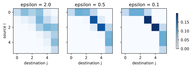
squared cost, LP optimum : 3.50000
epsilon = 2.0:     47 iterations, entropic cost = 4.06489, routes above 1e-3 = 25
epsilon = 0.5:    186 iterations, entropic cost = 3.56963, routes above 1e-3 = 14
epsilon = 0.1: 154325 iterations, entropic cost = 3.50002, routes above 1e-3 = 10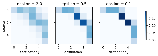
squared cost, LP optimum : 3.50000
epsilon = 2.0:     47 iterations, entropic cost = 4.06489, routes above 1e-3 = 25
epsilon = 0.5:    186 iterations, entropic cost = 3.56963, routes above 1e-3 = 14
epsilon = 0.1: 154325 iterations, entropic cost = 3.50002, routes above 1e-3 = 10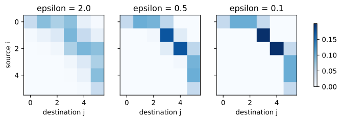
squared cost, LP optimum : 3.50000
epsilon = 2.0:     47 iterations, entropic cost = 4.06489, routes above 1e-3 = 25
epsilon = 0.5:    186 iterations, entropic cost = 3.56963, routes above 1e-3 = 14
epsilon = 0.1: 154325 iterations, entropic cost = 3.50002, routes above 1e-3 = 10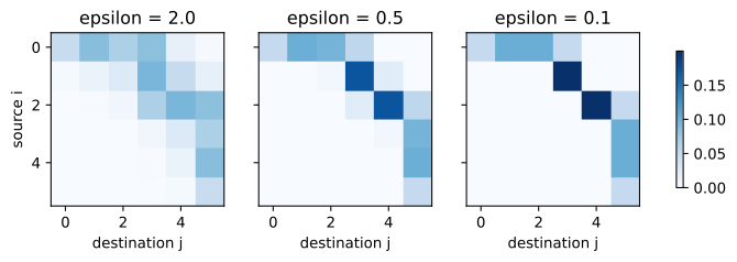
The linear program agrees on \(3.5\). At \(\varepsilon = 2\) the plan spreads each source’s mass over several destinations (\(25\) of the \(36\) routes carry more than \(10^{-3}\)), and its cost, \(4.06\), is well above the optimum. At \(\varepsilon = 0.5\) the plan has \(14\) routes and costs \(3.57\). At \(\varepsilon = 0.1\) only the ten routes of the monotone plan remain, and the cost, \(3.50002\), lies above the optimum by \(2 \times 10^{-5}\). In the heat maps a broad band sharpens into a staircase. The yardstick for \(\varepsilon\) is the difference in cost between competing routes, which is of order \(1\) on this grid, and a tenth of it was small enough.
The iteration counts show what this accuracy takes. About \(50\) iterations were enough at \(\varepsilon = 2\) and about \(190\) at \(\varepsilon = 0.5\), but \(\varepsilon = 0.1\) needed some \(150{,}000\). Between the last two runs \(\varepsilon\) fell fivefold and the work grew \(800\) times. Sinkhorn iterations are fast only as long as the plan may stay blurred (Exercise 8b measures the growth).
37.4.3 Fixed Kernels and Trained Critics
MMD and \(W_1\) divide the two requirements between them. The class behind a fixed kernel is small. MMD costs three averages, and the error of its estimate from \(N\) points is of order \(N^{-1/2}\) in any dimension (Gretton et al. 2012), but it sees only a few length scales. The functions of slope at most one see at every distance, which is what a model far from its data needs. They cannot jump, and yet in many dimensions they are still a very large class: between two samples in dimension \(n > 2\) the error of \(W_1\) is of order \(N^{-1/n}\) (Weed and Bach 2019). In \(100\) dimensions, halving that error takes \(2^{100}\) times the data. Nobody estimates \(W_1\) that way. A critic network searches a far smaller class than all functions of slope one, and Sinkhorn iterations serve where the problem is small.
Kernel and critic alike begin by drawing samples from the model. For some models that is the expensive step, and Section 37.5 asks what can be compared without it.
37.4.4 Summary
A little overlap does not bring the gradient back: for two unit Gaussians eight standard deviations apart, the Jensen–Shannon divergence and total variation have slopes near \(10^{-4}\). An integral probability metric compares instead how \(P\) and \(Q\) average a class of test functions, and the class decides both whether samples can estimate the gap and how far the comparison sees. Functions that are linear in fixed features give MMD, the distance between mean features: it is three kernel averages, which samples estimate with no critic, and it is blind beyond a few length scales. Functions of slope at most one give \(W_1\), the least mass times distance that turns one distribution into the other, which keeps a slope of one at every separation and is what the critic of a Wasserstein GAN estimates. On the line \(W_1\) is the area between the CDFs; elsewhere it needs a trained critic or, for small problems, Sinkhorn iterations on an entropically regularized plan.
37.4.5 Exercises
[code] MMD in closed form. Use the Gaussian integral Equation 37.4.4 for the RBF kernel with length scale \(\ell\), with \(P = \mathcal{N}(0, 1)\) and \(Q = \mathcal{N}(d, 1)\).
- Show that \(\textrm{MMD}^2 = \frac{2\ell}{\sqrt{\ell^2 + 2}} \big(1 - e^{-d^2/(2(\ell^2 + 2))}\big)\), and check that \(\ell = 1\) gives the \(\textrm{MMD}^2\) column of the opening table. Which length scale maximizes \(\textrm{MMD}^2\) for small shifts \(d\)? What happens as \(\ell \to 0\) and as \(\ell \to \infty\)?
- Evaluate the slope in \(d\) at \(d = 8\) for \(\ell = 1\), \(4\) and \(16\). What do the three values say about the length scale for a model that starts far from its data?
[code] Sampling error of the MMD estimate. At \(\ell = 1\) and \(d = 0.5\) the closed form \(\tfrac{2}{\sqrt{3}}\big(1 - e^{-d^2/6}\big)\) gives \(0.047\).
- Recompute
mmd2_unbiasedwith the RBF kernel on \(200\) fresh pairs of samples drawn likex_pandy_shift, withn = 250and withn = 1000, and compare the mean and the standard deviation of the estimates with the closed form. How does the standard deviation scale with the sample size? Is the value that your run of the MMD experiment printed within the spread? - Repeat for pairs drawn like
x_pandy_same. The standard deviation now scales differently. How, and why does this help a test of \(P = Q\)?
- Recompute
Rescaling and the data-processing inequality. An f-divergence is \(D_f(P\|Q) = \mathbb{E}_{x \sim Q}[f(p(x)/q(x))]\) for a convex \(f\) with \(f(1) = 0\), and it satisfies the data-processing inequality \(D_f(P\kappa \,\|\, Q\kappa) \leq D_f(P\|Q)\) for every channel \(\kappa\), that is, for every deterministic or random map applied to both distributions (Section 37.3.3.3). Apply the map \(x \mapsto 2x\) to both \(P\) and \(Q\).
- Show from the definition that no f-divergence changes under an invertible map, and that \(W_1\) doubles.
- Show that the RBF \(\textrm{MMD}^2\) at \(\ell = 1\) falls from \(0.047\) to \(0.036\) for \(\mathcal{N}(0, 1)\) against \(\mathcal{N}(0.5, 1)\), but rises from \(0.235\) to \(0.787\) for \(\delta_0\) against \(\delta_{0.5}\). Why does the data-processing inequality say nothing about MMD and \(W_1\)?
[code] One-dimensional transport. ● On the real line, \(W_1\) is the area between the CDFs Equation 37.4.7.
- For two empirical distributions on samples \(x_1, \ldots, x_N\) and \(y_1, \ldots, y_N\) of equal size, use the monotone plan of the proof to show that \(W_1 = \tfrac{1}{N} \sum_i |x_{(i)} - y_{(i)}|\), the mean absolute difference of the sorted values. Check this against the linear program of the six-point example on two random samples of size \(7\).
- Compute the sorted-sample \(W_1\) between
x_pandy_shiftand betweenx_pandy_sameof the MMD experiment. Then average it over \(20\) pairs of independent samples of size \(N\) from \(\mathcal{N}(0, 1)\), for \(N \in \{10^2, 10^3, 10^4\}\), and find the rate at which it decreases. The estimate is never negative. Why does this rule out unbiasedness when \(P = Q\)? - Change
q_wto \((0.40, 0.05, 0.05, 0.10, 0.10, 0.30)\), so that the two CDFs cross, and rerun the cell that computes \(W_1\). Build the test function \(g\) with \(g(0) = 0\) and slope \(\textrm{sign}\big(F_Q(t) - F_P(t)\big)\) between neighboring atoms, as in Step 4 of the proof, and check that \(\mathbb{E}_P[g] - \mathbb{E}_Q[g]\) equals the LP value. For every route \((i, j)\) that carries mass in the LP solutionplan_lp, compare \(g(x_i) - g(x_j)\) with \(|x_i - x_j|\). Why must the two agree on every such route for any optimal plan and any optimal test function? - Uniqueness under the squared cost. Suppose a plan moves mass from \(x\) to \(y'\) and from \(x'\) to \(y\), with \(x < x'\) and \(y < y'\), so that the two ribbons cross. Show that under the squared cost, sending the same mass from \(x\) to \(y\) and from \(x'\) to \(y'\) saves \(2(x' - x)(y' - y)\) per unit of mass, and deduce that the monotone plan is the only optimal one. What does the same exchange save under the cost \(|x - y|\) when all four moves go rightward? Find two ribbons that cross in
plan_lp, the plan that the linear program returned for the six-point example, and check your answer on them.
Optimal critics on the line. Step 4 of the proof of Equation 37.4.7 shows that a test function with slope \(g'(t) = \textrm{sign}\big(F_Q(t) - F_P(t)\big)\) attains \(W_1\).
- For \(P = \mathcal{N}(0, 1)\) and \(Q = \mathcal{N}(d, 1)\) with \(d > 0\), show that \(F_P > F_Q\) everywhere, so that Step 4 returns \(g(x) = -x\), the critic that the text found by inspection.
- For \(P = \mathcal{N}(0, 1)\) and \(Q = \mathcal{N}(0, 4)\), show that the two CDFs cross only at \(0\), that \(g(x) = -|x|\) is optimal, and that \(W_1 = \sqrt{2/\pi} \approx 0.80\). (For \(X \sim \mathcal{N}(0, \sigma^2)\), \(\mathbb{E}|X| = \sigma\sqrt{2/\pi}\).) The linear kernel reported \(0\) on this pair. Which way does the critic move the samples of \(Q\)?
- Let \(P = \tfrac12 \delta_0 + \tfrac12 \delta_3\) and \(Q = \tfrac12 \delta_1 + \tfrac12 \delta_3\). Find \(W_1(P, Q)\) and describe every optimal critic of the form used in Step 4. Then show in general that such a critic is optimal if and only if \(g'(t) = \textrm{sign}\big(F_Q(t) - F_P(t)\big)\) at almost every \(t\) with \(F_P(t) \neq F_Q(t)\), the points that mass has to cross, while its slope elsewhere is free.
- A WGAN critic is often trained with a penalty on \((|g'(x)| - 1)^2\) at points \(x\) between the data and the generated samples (Gulrajani et al. 2017). Explain this choice by (c). Which critics are optimal when \(P = Q\), and which of them does the penalty prefer? Section 16.4 shows what follows for training.
[code] \(W_2\) between Gaussians and the Fréchet distance. On the line the monotone plan \(X = F_P^{-1}(U)\), \(Y = F_Q^{-1}(U)\) is optimal for the squared cost.
- Show that for \(P = \mathcal{N}(\mu_1, \sigma_1^2)\) and \(Q = \mathcal{N}(\mu_2, \sigma_2^2)\) the monotone plan is \(Y = \mu_2 + (\sigma_2/\sigma_1)(X - \mu_1)\), and deduce that \(W_2^2(P, Q) = (\mu_1 - \mu_2)^2 + (\sigma_1 - \sigma_2)^2\). With the same plan, recover \(W_1 = |\mu_1 - \mu_2|\) for equal variances, the \(W_1\) column of the opening table.
- Let both standard deviations be \(\sigma\) and the means \(d\) apart. Then \(W_2^2 = d^2\) for every \(\sigma\), while the KL divergence between the two Gaussians is \(d^2/(2\sigma^2)\). What do the two report as \(\sigma \to 0\), when the Gaussians become the point masses of Table 37.3.1?
- In \(\mathbb{R}^n\) the squared \(W_2\) between \(\mathcal{N}(\boldsymbol{\mu}_1, \boldsymbol{\Sigma}_1)\) and \(\mathcal{N}(\boldsymbol{\mu}_2, \boldsymbol{\Sigma}_2)\) is the squared Fréchet distance \(\|\boldsymbol{\mu}_1 - \boldsymbol{\mu}_2\|^2 + \textrm{tr}\big(\boldsymbol{\Sigma}_1 + \boldsymbol{\Sigma}_2 - 2\,(\boldsymbol{\Sigma}_1^{1/2} \boldsymbol{\Sigma}_2 \boldsymbol{\Sigma}_1^{1/2})^{1/2}\big)\) (Dowson and Landau 1982). Check that it reduces to (a) for \(n = 1\) and, for diagonal covariance matrices, to the sum of (a) over the coordinates. Prove the diagonal case directly: the squared cost is a sum over coordinates, so no plan costs less than the sum of the coordinatewise optima, and the monotone plans of the coordinates together attain it.
- The Fréchet inception distance fits a Gaussian to each of two feature distributions and reports the squared Fréchet distance between the fits. Let \(P\) be the mixture \(0.7\,\mathcal{N}(-2, 0.6^2) + 0.3\,\mathcal{N}(2, 0.6^2)\) and \(Q = \mathcal{N}(-0.8, 3.72)\), which has the same mean and variance. What is the Fréchet distance between the two fits? Estimate \(W_2^2(P, Q)\) from \(10^5\) sorted draws of each (you should find about \(0.63\)). What does a Fréchet distance of zero certify, and what does it not?
[code] Entropic transport and Sinkhorn divergences. ●● Regularize the transport LP of the six-point example by the divergence from the independent plan,
\[ \textrm{OT}_\varepsilon(P, Q) = \min_{\gamma}\, \sum_{i, j} \gamma_{ij} C_{ij} + \varepsilon\, D_{\textrm{KL}}\big(\gamma \,\|\, p\, q^\top\big), \]
where \(\gamma\) ranges over the plans with row sums \(p\) and column sums \(q\).
- Show that \(D_{\textrm{KL}}(\gamma \,\|\, p\, q^\top) = -H(\gamma) + H(P) + H(Q)\) for every such plan, where \(H\) denotes the entropy, so that
sinkhornreturns the minimizer. Show that \(\textrm{OT}_\varepsilon(P, Q) \to \sum_{i, j} p_i q_j C_{ij}\) as \(\varepsilon \to \infty\), and that \(\textrm{OT}_\varepsilon(P, P) > 0\) for every \(\varepsilon > 0\) unless \(P\) is a point mass. With \(C_{ij} = |x_i - x_j|\), show that the distributions \(P\) on the atoms that minimize the limit \(\sum_{i, j} p_i q_j C_{ij}\) put all their mass on medians of \(Q\), forq_wthe atoms \(3\) and \(4\). What would a model trained on \(\textrm{OT}_\varepsilon\) with a large \(\varepsilon\) learn? - The Sinkhorn divergence \(S_\varepsilon(P, Q) = \textrm{OT}_\varepsilon(P, Q)
- \tfrac{1}{2} \textrm{OT}_\varepsilon(P, P)
- \tfrac{1}{2} \textrm{OT}_\varepsilon(Q, Q)\) removes this bias (Genevay et al. 2018; Feydy et al. 2019). Compute \(S_\varepsilon(P, Q)\) for
p_wandq_wwith the absolute costCat \(\varepsilon \in \{10^{-3}, 10^{-2}, \ldots, 10^3\}\). At \(\varepsilon = 10^{-3}\) the entries of \(\mathbf{K}\) underflow, so carry out the Sinkhorn updates on \(\log \mathbf{a}\) and \(\log \mathbf{b}\) there, withscipy.special.logsumexp. Check that \(S_\varepsilon\) approaches \(W_1\) as \(\varepsilon \to 0\) and \(\tfrac{1}{2} \mathcal{E}(P, Q)\) as \(\varepsilon \to \infty\), where \(\mathcal{E}(P, Q) = 2\mathbb{E}|X - Y| - \mathbb{E}|X - X'| - \mathbb{E}|Y - Y'|\) is the energy distance (Székely and Rizzo 2013), the expression Equation 37.4.3 with \(-|x - y|\) in place of the kernel. Derive the second limit from (a).
- Show that \(D_{\textrm{KL}}(\gamma \,\|\, p\, q^\top) = -H(\gamma) + H(P) + H(Q)\) for every such plan, where \(H\) denotes the entropy, so that
[code] Sinkhorn iterations at small \(\varepsilon\). ● Use
sinkhorn,p_wandq_wof the six-point example.- Stopping early. Call
sinkhornwith the squared costC2at \(\varepsilon = 0.1\) andmax_iters=5000, so that the loop ends before the column sums have settled. The cost that it returns is below the optimum \(3.5\). Print the column sums of the returned matrix minusq_w. Which destinations receive too little, and why does that lower the cost? Why can no matrix with row sumsp_wand column sumsq_wcost less than \(3.5\)? - The number of iterations. Count the iterations that
sinkhornneeds withC2at \(\varepsilon \in \{2, 1, 0.5, 0.3, 0.2, 0.15, 0.1\}\), and plot the logarithm of the count against \(1/\varepsilon\). What kind of growth do the points at small \(\varepsilon\) show, and what count does it predict for \(\varepsilon = 0.05\)? - Ties. Under the absolute cost
Cevery plan that moves mass only rightward is optimal forp_wandq_w. RunsinkhornwithCat \(\varepsilon = 0.1\) and \(0.02\). How many routes carry mass? Show that the limit plan has the form \(\gamma_{ij} = a_i b_j\) for \(j \geq i\) and \(0\) otherwise. On plans the regularizer is \(-\varepsilon\) times the entropy plus a constant. Use this to explain why the limit is the plan of largest entropy among the optimal plans.
- Stopping early. Call