%matplotlib inline
from d2l import torch as d2l
import numpy as np26.4 Constrained Optimization and Duality
Constraints appear in projected and clipped updates, trust regions, support vector machines, and regularization. This section develops equality and inequality constraints, the Karush–Kuhn–Tucker conditions, projected gradient descent, Lagrangian duality, and strong duality (Boyd and Vandenberghe 2004). Worked examples derive the SVM dual, solve a water-filling problem by bisection, and exhibit a nonconvex duality gap.
At an unconstrained minimum the gradient vanishes. At a constrained minimum it may be nonzero, but no feasible infinitesimal direction can decrease the objective. Lagrange multipliers, the KKT conditions, and fixed points of projected gradient descent express this condition for different constraint sets.
We lean on Section 25.2 (gradients, level sets, and the tangency condition used below), Section 26.1 (stationarity and the descent lemma), and Section 26.3 (convex sets and functions, required for KKT sufficiency and strong duality). The standard reference is Boyd and Vandenberghe (2004), chapter 5; Nocedal and Wright (2006) gives the numerical view. The code in this section is plain NumPy, because the algorithms have compact NumPy implementations; we load the d2l module once for plotting.
%matplotlib inline
from d2l import tensorflow as d2l
import numpy as np%matplotlib inline
from d2l import jax as d2l
import numpy as np%matplotlib inline
from d2l import mxnet as d2l
import numpy as np26.4.1 Equality Constraints and Lagrange Multipliers
26.4.1.1 Feasible Directions at an Equality-Constrained Minimum
Consider the simplest constrained problem: minimize a smooth \(f : \mathbb{R}^n \to \mathbb{R}\) over the surface defined by one smooth equality constraint,
\[ \min_{\mathbf{x}}\; f(\mathbf{x}) \quad \textrm{subject to} \quad g(\mathbf{x}) = 0. \]
The geometric argument requires the regularity condition \(\nabla g(\mathbf{x}^\star)\ne\mathbf{0}\). It ensures that the feasible set is locally a smooth surface with a well-defined tangent space. Without it, the tangency conclusion may fail; an adjacent counterexample follows the proposition.
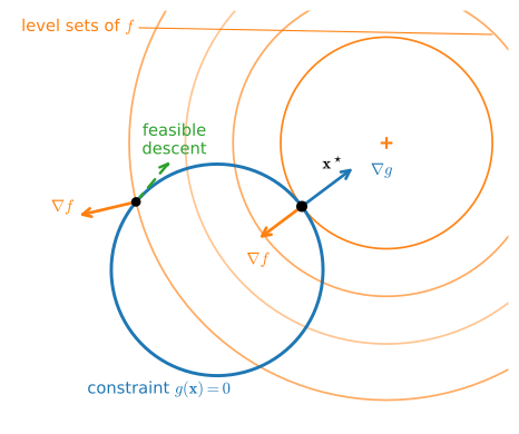
Section 25.2 supplies the geometric interpretation: the admissible moves from a feasible point are, to first order, directions tangent to the surface \(\{g = 0\}\), and at a regular constrained optimum the level set of \(f\) is tangent to the constraint surface. Figure 26.4.1 shows why tangency is forced. At a feasible point where a level curve of \(f\) crosses the constraint curve, the gradient \(\nabla f\) has a nonzero component along the constraint, so moving along the constraint opposite that component decreases \(f\) while staying feasible. A feasible descent direction exists, and the point cannot be optimal. Only where the level curve is tangent to the constraint does every feasible direction become neutral to first order, and tangency of the curves is parallelism of their normals: \(\nabla f\) must be a multiple of \(\nabla g\).
Proposition (Lagrange condition). Let \(f\) and \(g\) be continuously differentiable, and let \(\mathbf{x}^\star\) be a local minimum of \(f\) on \(\{\mathbf{x} : g(\mathbf{x}) = 0\}\) at which \(\nabla g(\mathbf{x}^\star) \neq \mathbf{0}\). Then there is a unique scalar \(\nu^\star\), called the Lagrange multiplier, such that
\[ \nabla f(\mathbf{x}^\star) + \nu^\star\,\nabla g(\mathbf{x}^\star) = \mathbf{0}. \tag{26.4.1}\]
Proof. The first-order feasible directions at \(\mathbf{x}^\star\) are the tangent directions \(\mathbf{v}\) with \(\nabla g(\mathbf{x}^\star)^\top\mathbf{v} = 0\). Because \(\nabla g(\mathbf{x}^\star) \neq \mathbf{0}\), the implicit function theorem (stated in Section 25.3.4.6, and taken on faith at this chapter’s level of rigor) makes the feasible set a genuine smooth surface near \(\mathbf{x}^\star\): every such \(\mathbf{v}\) is the velocity of some curve \(\mathbf{x}(t)\) that stays on the surface with \(\mathbf{x}(0) = \mathbf{x}^\star\), \(\dot{\mathbf{x}}(0) = \mathbf{v}\). Since \(\mathbf{x}^\star\) minimizes \(f\) along each such curve, and the curve can be traversed in both directions \(\pm\mathbf{v}\), the derivative at \(t = 0\) must vanish rather than merely be nonnegative:
\[ \left.\frac{d}{dt} f(\mathbf{x}(t))\right|_{t=0} = \nabla f(\mathbf{x}^\star)^\top \mathbf{v} = 0 \quad\textrm{for every } \mathbf{v} \perp \nabla g(\mathbf{x}^\star). \]
So \(\nabla f(\mathbf{x}^\star)\) is orthogonal to the entire tangent hyperplane \(\{\mathbf{v} : \nabla g^\top\mathbf{v} = 0\}\), whose orthogonal complement is the line spanned by \(\nabla g(\mathbf{x}^\star)\) (Section 24.1). Hence \(\nabla f(\mathbf{x}^\star) = -\nu^\star \nabla g(\mathbf{x}^\star)\) for exactly one scalar \(\nu^\star\). \(\blacksquare\)
This is the tangency condition of Section 25.2, which wrote it as \(\nabla f = \lambda\,\nabla g\); the two conventions agree with \(\nu = -\lambda\), and the plus sign here is the one the Lagrangian below makes natural.
The hypothesis \(\nabla g(\mathbf{x}^\star) \neq \mathbf{0}\) is called a constraint qualification, and it can fail. Minimize \(f(\mathbf{x}) = x_1\) subject to \(g(\mathbf{x}) = x_1^2 + x_2^2 = 0\): the feasible set is the single point \(\mathbf{0}\), which is therefore the minimum, yet \(\nabla f(\mathbf{0}) = (1, 0)\) while \(\nabla g(\mathbf{0}) = \mathbf{0}\): no multiplier exists. The constraint set has collapsed to a point, the “surface” is not a surface, so the tangent-space argument does not apply. Invoking multipliers therefore requires verifying that the constraint gradients do not degenerate at the optimum.
26.4.1.2 The Lagrangian
The two optimality requirements (parallel gradients and feasibility) combine into stationarity of a single function of more variables, the Lagrangian
\[ \mathcal{L}(\mathbf{x}, \nu) = f(\mathbf{x}) + \nu\, g(\mathbf{x}), \tag{26.4.2}\]
since
\[ \nabla_{\mathbf{x}} \mathcal{L} = \nabla f + \nu \nabla g = \mathbf{0} \qquad\textrm{and}\qquad \frac{\partial \mathcal{L}}{\partial \nu} = g(\mathbf{x}) = 0 \]
are exactly Equation 26.4.1 and the constraint. The constrained problem in \(\mathbf{x}\) is represented as an unconstrained stationarity problem in \((\mathbf{x}, \nu)\); the multiplier is a coordinate of the optimality condition. With several equality constraints \(h_j(\mathbf{x}) = 0\), \(j = 1, \ldots, p\), each gets its own multiplier, \(\mathcal{L} = f + \sum_j \nu_j h_j\), and the same argument (now requiring the \(\nabla h_j(\mathbf{x}^\star)\) to be linearly independent) puts \(\nabla f(\mathbf{x}^\star)\) in the span of the constraint gradients: the objective’s gradient is balanced by a combination of the constraint normals, with nothing left over along any feasible direction.
26.4.1.3 Worked Example: Closest Point on a Hyperplane
Minimize \(f(\mathbf{x}) = \mathbf{x}^\top\mathbf{x}\) subject to \(h(\mathbf{x}) = \mathbf{a}^\top\mathbf{x} - b = 0\): the point of a hyperplane nearest the origin. Stationarity of \(\mathcal{L} = \mathbf{x}^\top\mathbf{x} + \nu(\mathbf{a}^\top\mathbf{x} - b)\) gives \(2\mathbf{x} + \nu\mathbf{a} = \mathbf{0}\), so \(\mathbf{x} = -\tfrac{\nu}{2}\mathbf{a}\): the solution lies along the normal \(\mathbf{a}\). Feasibility fixes the scale, \(\nu^\star = -2b/\|\mathbf{a}\|^2\), hence
\[ \mathbf{x}^\star = \frac{b}{\|\mathbf{a}\|^2}\,\mathbf{a}, \]
recovering the projection formula of Section 24.1. The multiplier also has a sensitivity interpretation: the optimal value is \(p^\star(b) = b^2/\|\mathbf{a}\|^2\), and \(\partial p^\star / \partial b = 2b/\|\mathbf{a}\|^2 = -\nu^\star\). The multiplier measures the derivative of the optimal value with respect to the constraint parameter; this is called a shadow price. The general result appears in Section 26.4.4.
26.4.2 Inequality Constraints and the KKT Conditions
26.4.2.1 Active and Inactive Constraints
Most constraints in practice are one-sided: a norm at most \(r\), a probability at least \(0\), a budget not exceeded. Consider
\[ \min_{\mathbf{x}}\; f(\mathbf{x}) \quad \textrm{subject to} \quad g_i(\mathbf{x}) \le 0,\; i = 1, \ldots, m. \]
At the optimum each inequality is in one of two regimes. Either \(g_i(\mathbf{x}^\star) < 0\): the constraint is inactive, the optimum lies strictly inside its region, and locally the constraint might as well not exist. Or \(g_i(\mathbf{x}^\star) = 0\): the constraint is active and behaves like an equality, and contributes to first-order stationarity.
A worked example shows both regimes at once. Project a point onto a ball: minimize \(\tfrac12\|\mathbf{x} - \mathbf{x}_0\|^2\) subject to \(g(\mathbf{x}) = \tfrac12(\|\mathbf{x}\|^2 - r^2) \le 0\). Stationarity of \(\mathcal{L} = \tfrac12\|\mathbf{x} - \mathbf{x}_0\|^2 + \lambda g(\mathbf{x})\) gives \((\mathbf{x} - \mathbf{x}_0) + \lambda\mathbf{x} = \mathbf{0}\), i.e. \(\mathbf{x} = \mathbf{x}_0 / (1 + \lambda)\): the constrained solution is a radial rescaling of the input vector. If \(\|\mathbf{x}_0\| \le r\) the constraint is inactive, \(\lambda^\star = 0\) and \(\mathbf{x}^\star = \mathbf{x}_0\); if \(\|\mathbf{x}_0\| > r\) it is active, \(\|\mathbf{x}^\star\| = r\) forces \(\lambda^\star = \|\mathbf{x}_0\|/r - 1 > 0\), and
\[ \mathbf{x}^\star = \frac{\mathbf{x}_0}{\max\left(1,\; \|\mathbf{x}_0\|/r\right)}. \]
Gradient clipping applies this projection to the update vector (Pascanu et al. 2013). And note the sign of the active multiplier: \(\lambda^\star > 0\), never negative. The nonnegativity of an inequality multiplier distinguishes it from an unrestricted equality multiplier and enforces the orientation of the active constraint normal.
26.4.2.2 The Karush–Kuhn–Tucker Conditions
Assembling the general problem with both kinds of constraints,
\[ \min_{\mathbf{x}}\; f(\mathbf{x}) \quad \textrm{subject to} \quad g_i(\mathbf{x}) \le 0,\; i = 1, \ldots, m, \qquad h_j(\mathbf{x}) = 0,\; j = 1, \ldots, p, \tag{26.4.3}\]
the Lagrangian acquires a multiplier per constraint,
\[ \mathcal{L}(\mathbf{x}, \boldsymbol{\lambda}, \boldsymbol{\nu}) = f(\mathbf{x}) + \sum_{i=1}^m \lambda_i\, g_i(\mathbf{x}) + \sum_{j=1}^p \nu_j\, h_j(\mathbf{x}), \qquad \lambda_i \ge 0, \tag{26.4.4}\]
and the first-order optimality conditions are the four Karush–Kuhn–Tucker (KKT) conditions (Karush 1939; Kuhn and Tucker 1951):
\[ \begin{aligned} &\textrm{stationarity:} && \nabla f(\mathbf{x}^\star) + \textstyle\sum_i \lambda_i^\star \nabla g_i(\mathbf{x}^\star) + \sum_j \nu_j^\star \nabla h_j(\mathbf{x}^\star) = \mathbf{0}, \\ &\textrm{primal feasibility:} && g_i(\mathbf{x}^\star) \le 0, \qquad h_j(\mathbf{x}^\star) = 0, \\ &\textrm{dual feasibility:} && \lambda_i^\star \ge 0, \\ &\textrm{complementary slackness:} && \lambda_i^\star\, g_i(\mathbf{x}^\star) = 0 \quad \textrm{for every } i. \end{aligned} \tag{26.4.5}\]
Stationarity balances the objective and constraint gradients; primal feasibility restates the constraints; dual feasibility requires nonnegative inequality multipliers. The fourth, complementary slackness, says that for each constraint, at least one of \(\lambda_i^\star\) and \(g_i(\mathbf{x}^\star)\) is zero: a constraint is either active (\(g_i = 0\), multiplier free to be positive) or priced at zero (\(\lambda_i = 0\), constraint slack and locally irrelevant). It identifies the active set: in a KKT solution, zero and nonzero multipliers indicate which constraints contribute to stationarity. In the ball projection, complementary slackness is precisely the case split we did by hand.
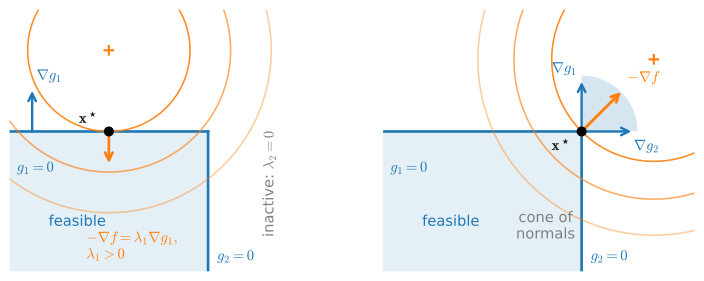
Figure 26.4.2 draws stationarity plus dual feasibility: at the optimum, \(-\nabla f\) is a nonnegative combination of the active constraints’ outward normals. Equivalently, it belongs to the normal cone generated by the active constraints; inactive constraints contribute nothing.
How strong are these conditions? In general they are necessary: multipliers satisfying Equation 26.4.5 exist at any local minimum that satisfies a constraint qualification (the standard one, LICQ, asks the active constraints’ gradients to be linearly independent, the inequality analogue of \(\nabla g \neq \mathbf{0}\) above); see Nocedal and Wright (2006), chapter 12, for the proof. They are not sufficient: a non-convex problem can have KKT points that are saddles or maxima (Exercise 3). Under convexity, the conditions are also sufficient, as the following proof shows.
Proposition (KKT sufficiency under convexity). In problem Equation 26.4.3, let \(f\) and every \(g_i\) be convex and differentiable and every \(h_j\) affine. If \((\mathbf{x}^\star, \boldsymbol{\lambda}^\star, \boldsymbol{\nu}^\star)\) satisfies the KKT conditions Equation 26.4.5, then \(\mathbf{x}^\star\) is a global minimum.
Proof. The function \(\varphi(\mathbf{x}) = \mathcal{L}(\mathbf{x}, \boldsymbol{\lambda}^\star, \boldsymbol{\nu}^\star)\) is convex: it is a nonnegative combination of convex functions plus affine terms (Section 26.3). Stationarity says \(\nabla\varphi(\mathbf{x}^\star) = \mathbf{0}\), so \(\mathbf{x}^\star\) is a global minimizer of \(\varphi\). Now take any feasible \(\mathbf{x}\). Since \(\lambda_i^\star \ge 0\), \(g_i(\mathbf{x}) \le 0\), and \(h_j(\mathbf{x}) = 0\),
\[ f(\mathbf{x}) \;\ge\; f(\mathbf{x}) + \sum_i \lambda_i^\star g_i(\mathbf{x}) + \sum_j \nu_j^\star h_j(\mathbf{x}) = \varphi(\mathbf{x}) \;\ge\; \varphi(\mathbf{x}^\star) = f(\mathbf{x}^\star), \]
where the last equality uses complementary slackness (\(\sum_i \lambda_i^\star g_i(\mathbf{x}^\star) = 0\)) and feasibility (\(h_j(\mathbf{x}^\star) = 0\)). \(\blacksquare\)
For convex problems, the KKT system is necessary (under a constraint qualification we will meet as Slater’s condition) and sufficient. This extends unconstrained first-order stationarity to constrained problems and is used in the examples below.
26.4.3 Projections and Projected Gradient Descent
The KKT conditions characterize optima; projection provides a corresponding algorithmic update. Take the ordinary gradient step, and if it leaves the feasible set, project to the nearest feasible point.
26.4.3.1 Projection onto a Convex Set
For a closed convex set \(C \subseteq \mathbb{R}^n\), the projection of \(\mathbf{y}\) onto \(C\) is the nearest feasible point,
\[ \Pi_C(\mathbf{y}) = \mathop{\mathrm{argmin}}_{\mathbf{x} \in C}\; \tfrac12 \|\mathbf{x} - \mathbf{y}\|^2. \]
A minimizer exists whenever \(C\) is nonempty: we may restrict the search to the intersection of \(C\) with a large closed ball around \(\mathbf{y}\), which is compact because \(C\) is closed, and the continuous objective attains its minimum there. It is unique because the objective is strictly convex. So \(\Pi_C\) is a well-defined map. Both examples we have computed are projections: onto a hyperplane in Section 26.4.1, onto a ball (the clipping formula) in Section 26.4.2.
Projections onto closed convex sets have a useful first-order characterization. The point \(\hat{\mathbf{x}} = \Pi_C(\mathbf{y})\) minimizes the convex function \(\tfrac12\|\mathbf{x} - \mathbf{y}\|^2\) over the convex set \(C\), and “no feasible descent” over a convex set takes an especially simple form: for any \(\mathbf{x} \in C\) the whole segment from \(\hat{\mathbf{x}}\) to \(\mathbf{x}\) is feasible, so the directional derivative along it must be nonnegative, giving \((\hat{\mathbf{x}} - \mathbf{y})^\top(\mathbf{x} - \hat{\mathbf{x}}) \ge 0\), i.e.
\[ \left(\mathbf{y} - \Pi_C(\mathbf{y})\right)^\top \left(\mathbf{x} - \Pi_C(\mathbf{y})\right) \;\le\; 0 \qquad \textrm{for all } \mathbf{x} \in C. \tag{26.4.6}\]
Geometrically: the residual \(\mathbf{y} - \Pi_C(\mathbf{y})\) makes an obtuse angle with every feasible direction; the set \(C\) lies entirely on the far side of the supporting hyperplane through \(\Pi_C(\mathbf{y})\) with normal \(\mathbf{y} - \Pi_C(\mathbf{y})\). The inequality is also sufficient: if \(\hat{\mathbf{x}} \in C\) satisfies it, apply the first-order convexity condition Equation 26.3.3 to \(\varphi(\mathbf{x}) = \tfrac12\|\mathbf{x} - \mathbf{y}\|^2\), whose gradient at \(\hat{\mathbf{x}}\) is \(\hat{\mathbf{x}} - \mathbf{y}\): for every \(\mathbf{x} \in C\), \(\varphi(\mathbf{x}) \ge \varphi(\hat{\mathbf{x}}) + (\hat{\mathbf{x}} - \mathbf{y})^\top(\mathbf{x} - \hat{\mathbf{x}}) \ge \varphi(\hat{\mathbf{x}})\), so \(\hat{\mathbf{x}} = \Pi_C(\mathbf{y})\). Thus Equation 26.4.6 characterizes the projection. This inequality implies nonexpansiveness, which is used in projected-method analysis.
Proposition (projections are nonexpansive). For a closed convex set \(C\) and all \(\mathbf{x}, \mathbf{y} \in \mathbb{R}^n\),
\[ \|\Pi_C(\mathbf{x}) - \Pi_C(\mathbf{y})\| \;\le\; \|\mathbf{x} - \mathbf{y}\|. \]
Proof. Write \(\mathbf{u} = \Pi_C(\mathbf{x})\), \(\mathbf{v} = \Pi_C(\mathbf{y})\). Apply Equation 26.4.6 twice: at \(\mathbf{x}\) with test point \(\mathbf{v}\), and at \(\mathbf{y}\) with test point \(\mathbf{u}\):
\[ (\mathbf{x} - \mathbf{u})^\top(\mathbf{v} - \mathbf{u}) \le 0, \qquad (\mathbf{y} - \mathbf{v})^\top(\mathbf{u} - \mathbf{v}) \le 0. \]
Adding them gives \((\mathbf{x} - \mathbf{y} - (\mathbf{u} - \mathbf{v}))^\top(\mathbf{v} - \mathbf{u}) \le 0\), which rearranges to
\[ \|\mathbf{u} - \mathbf{v}\|^2 \;\le\; (\mathbf{x} - \mathbf{y})^\top (\mathbf{u} - \mathbf{v}) \;\le\; \|\mathbf{x} - \mathbf{y}\|\, \|\mathbf{u} - \mathbf{v}\| \]
by the Cauchy–Schwarz inequality Equation 24.1.4; divide by \(\|\mathbf{u} - \mathbf{v}\|\) (the claim is trivial when it is zero). \(\blacksquare\)
Projection onto a convex set does not increase distances. For a nonconvex set, the projection can be multivalued or discontinuous; even a pair of points gives nearby inputs whose selected projections are far apart.
26.4.3.2 Projected Gradient Descent
Projected gradient descent (PGD) interleaves a gradient step with a projection:
\[ \mathbf{x}_{t+1} = \Pi_C\left(\mathbf{x}_t - \eta\, \nabla f(\mathbf{x}_t)\right). \tag{26.4.7}\]
For a nonempty closed convex set \(C\), a convex \(L\)-smooth objective, and \(\eta=1/L\), PGD has an \(O(1/k)\) objective-value rate (Nesterov 2018). Nonexpansiveness of the projection is part of that analysis. More generally, for differentiable \(f\), convex \(C\), and any \(\eta>0\), the fixed points of Equation 26.4.7 are exactly the first-order stationary points for the constrained problem. Indeed, \(\mathbf{x}^\star = \Pi_C(\mathbf{x}^\star - \eta \nabla f(\mathbf{x}^\star))\) holds iff plugging \(\mathbf{y} = \mathbf{x}^\star - \eta\nabla f(\mathbf{x}^\star)\) into Equation 26.4.6 does, which after cancelling \(\mathbf{x}^\star\) reads
\[ \nabla f(\mathbf{x}^\star)^\top (\mathbf{x} - \mathbf{x}^\star) \;\ge\; 0 \qquad \textrm{for all } \mathbf{x} \in C \]
This is the constrained first-order condition, reducing to \(\nabla f = \mathbf{0}\) when \(C = \mathbb{R}^n\). If \(f\) is convex, the condition is also sufficient for global optimality; if \(f\) is nonconvex, it certifies only stationarity. Under a constraint qualification such as Slater’s (introduced below), it is equivalent to the KKT conditions when \(C\) is described by convex inequalities. Convexity of \(C\) is also essential: for a nonconvex set the projection may be multivalued and the fixed-point equivalence can fail.
Non-negativity constraints use projection onto the orthant, and max-norm weight constraints project rows onto balls after the update. Gradient norm clipping also projects the gradient vector onto a ball, but is not generally PGD for a constraint on the parameters. PGD is practical whenever \(\Pi_C\) is cheap, which brings us to the projection behind sparse attention.
26.4.3.3 Projection onto the Simplex
The probability simplex \(\Delta = \{\mathbf{x} : \mathbf{x} \ge 0,\; \sum_i x_i = 1\}\) is where distributions live, and projecting onto it,
\[ \min_{\mathbf{x}}\; \tfrac12\|\mathbf{x} - \mathbf{y}\|^2 \quad \textrm{subject to} \quad \textstyle\sum_i x_i = 1, \;\; -x_i \le 0, \]
is a small quadratic program (QP: convex quadratic objective with affine constraints). The KKT conditions reduce its solution to finding one scalar. With multiplier \(\tau\) for the sum and \(\lambda_i \ge 0\) for each sign constraint, stationarity reads \(x_i - y_i + \tau - \lambda_i = 0\). Complementary slackness splits the coordinates: where \(x_i > 0\) we get \(\lambda_i = 0\) and \(x_i = y_i - \tau\); where \(x_i = 0\), dual feasibility \(\lambda_i = \tau - y_i \ge 0\) says exactly that \(y_i \le \tau\). Both cases combine as
\[ x_i^\star = \max(y_i - \tau,\, 0), \qquad \textrm{with } \tau \textrm{ set by } \sum_i \max(y_i - \tau,\, 0) = 1. \tag{26.4.8}\]
Every coordinate is shifted down by the same \(\tau\) and clipped at zero; the normalization condition determines the threshold. The left side of the \(\tau\)-equation is continuous, piecewise linear, and strictly decreasing where positive, so the threshold is unique and found by sorting: with \(u_1 \ge \cdots \ge u_n\) the sorted entries of \(\mathbf{y}\), the active set is a top-\(k\) prefix, and \(\tau = (\sum_{j \le k} u_j - 1)/k\) for the largest \(k\) keeping \(u_k > \tau\), an \(O(n \log n)\) algorithm (Held et al. 1974; Duchi et al. 2008). Applied to scores instead of a softmax, this map is exactly sparsemax (Martins and Astudillo 2016): unlike softmax it produces genuinely sparse attention weights, with complementary slackness determining which entries are zero. More broadly, attention itself can be read as a regularized argmax over the simplex: softmax arises from an entropy regularizer, and sparsemax from the squared Euclidean distance used here (Niculae and Blondel 2017). The cell below implements the sort-and-threshold projection, reconstructs all the multipliers, and checks every KKT residual numerically, plus a sanity check that no random feasible point does better.
def project_simplex(y):
    """Project y onto the probability simplex by sort-and-threshold."""
    u = np.sort(y)[::-1]                       # sorted descending
    css = np.cumsum(u) - 1.0                   # cumulative sums minus budget
    k = np.nonzero(u * np.arange(1, len(y) + 1) > css)[0][-1]
    tau = css[k] / (k + 1.0)                   # multiplier of sum(x) = 1
    return np.maximum(y - tau, 0.0), tau

rng = np.random.default_rng(0)
y = rng.normal(size=6)
x, tau = project_simplex(y)
lam = np.maximum(0.0, tau - y)                 # multipliers of x >= 0
print('x* =', x.round(4), ' sum =', f'{x.sum():.6f}')
print('KKT residuals: stationarity', f'{np.abs(x - y + tau - lam).max():.1e}',
      '| comp. slack', f'{np.abs(lam * x).max():.1e}',
      '| dual feas.', f'{lam.min():.1e}')
# Optimality check: x* beats 10^5 random feasible points
z = rng.exponential(size=(100000, len(y)))
z /= z.sum(axis=1, keepdims=True)              # random points on the simplex
print('f(x*) =', f'{0.5 * ((x - y)**2).sum():.6f}',
      '<= best random feasible', f'{(0.5 * ((z - y)**2).sum(axis=1)).min():.6f}')
x* = [0.0676 0. 0.5823 0.0467 0. 0.3034] sum = 1.000000
KKT residuals: stationarity 5.6e-17 | comp. slack 0.0e+00 | dual feas. 0.0e+00
f(x*) = 0.158962 <= best random feasible 0.162139The stationarity, complementary-slackness, and dual-feasibility residuals are at machine precision. Two of the six coordinates are exactly zero; their sign constraints are active and have strictly positive multipliers. The KKT case analysis yields the algorithm, and its residuals verify the solution.
26.4.4 The Dual Problem
26.4.4.1 The Lagrange Dual Function
So far, multipliers were unknowns solved alongside \(\mathbf{x}\). Duality treats them as optimization variables. Fix \((\boldsymbol{\lambda}, \boldsymbol{\nu})\) with \(\boldsymbol{\lambda} \succeq 0\) (elementwise, in the vector sense of the \(\succeq\) convention of Section 26.3) and minimize the Lagrangian Equation 26.4.4 over \(\mathbf{x}\) unconstrained:
\[ g(\boldsymbol{\lambda}, \boldsymbol{\nu}) = \inf_{\mathbf{x}}\; \mathcal{L}(\mathbf{x}, \boldsymbol{\lambda}, \boldsymbol{\nu}). \tag{26.4.9}\]
The infimum is over all of \(\mathbb{R}^n\) and need not be attained or even finite: for many multiplier values the Lagrangian is unbounded below and \(g(\boldsymbol{\lambda}, \boldsymbol{\nu}) = -\infty\). The dual problem below implicitly maximizes over the region where \(g\) is finite (its effective domain); in the SVM dual, this mechanism produces an equality constraint.
The Lagrange dual function has two properties that require no assumptions on \(f\), \(g_i\), or \(h_j\).
Proposition (the dual function is concave). For any primal problem, \(g(\boldsymbol{\lambda}, \boldsymbol{\nu})\) in Equation 26.4.9 is concave.
Proof. For each fixed \(\mathbf{x}\), the map \((\boldsymbol{\lambda}, \boldsymbol{\nu}) \mapsto \mathcal{L}(\mathbf{x}, \boldsymbol{\lambda}, \boldsymbol{\nu})\) is affine: the multipliers enter linearly. The dual function is the pointwise infimum of this family of affine functions, and a pointwise infimum of affine functions is concave: its hypograph (the set of points on or below its graph, the mirror image of the epigraph of Section 26.3) is the intersection of the half-spaces below the affine functions, an intersection of convex sets. \(\blacksquare\)
Proposition (weak duality). If \(\mathbf{x}\) is feasible for Equation 26.4.3 and \(\boldsymbol{\lambda} \succeq 0\), then \(g(\boldsymbol{\lambda}, \boldsymbol{\nu}) \le f(\mathbf{x})\). Consequently
\[ d^\star \;=\; \sup_{\boldsymbol{\lambda} \succeq 0,\, \boldsymbol{\nu}} g(\boldsymbol{\lambda}, \boldsymbol{\nu}) \;\le\; \inf_{\mathbf{x}\ \textrm{feasible}} f(\mathbf{x}) \;=\; p^\star. \tag{26.4.10}\]
Proof. For feasible \(\mathbf{x}\): each \(\lambda_i g_i(\mathbf{x}) \le 0\) (nonnegative times nonpositive) and each \(\nu_j h_j(\mathbf{x}) = 0\), so
\[ g(\boldsymbol{\lambda}, \boldsymbol{\nu}) \;\le\; \mathcal{L}(\mathbf{x}, \boldsymbol{\lambda}, \boldsymbol{\nu}) \;=\; f(\mathbf{x}) + \sum_i \lambda_i g_i(\mathbf{x}) + \sum_j \nu_j h_j(\mathbf{x}) \;\le\; f(\mathbf{x}). \]
Take the supremum over \((\boldsymbol{\lambda}, \boldsymbol{\nu})\) on the left and the infimum over feasible \(\mathbf{x}\) on the right. \(\blacksquare\)
The dual problem maximizes \(g\) over \(\boldsymbol{\lambda} \succeq 0\), and it is always a convex optimization problem (maximizing a concave function over a convex set), even when the primal is non-convex. Its optimal value \(d^\star\) is always a certified lower bound on the primal optimum. Every dual feasible point provides a certificate: if \((\boldsymbol{\lambda}, \boldsymbol{\nu})\) satisfies \(g(\boldsymbol{\lambda}, \boldsymbol{\nu}) = 17\), then there is no feasible \(\mathbf{x}\) with \(f(\mathbf{x}) < 17\). The difference \(p^\star - d^\star \ge 0\) is the duality gap between the primal and dual optimal values.
26.4.4.2 Strong Duality and Slater’s Condition
Slater’s condition gives a standard sufficient condition for a convex problem to have zero duality gap: it requires one strictly feasible point.
Proposition (Slater’s condition implies strong duality). Suppose the problem Equation 26.4.3 is convex (\(f\), \(g_i\) convex, \(h_j\) affine) and there exists a strictly feasible point: some \(\bar{\mathbf{x}}\) with \(g_i(\bar{\mathbf{x}}) < 0\) for all \(i\) and \(h_j(\bar{\mathbf{x}}) = 0\). Then \(d^\star = p^\star\), and the dual optimum is attained. The condition is due to Slater (1950); for the proof see Boyd and Vandenberghe (2004), section 5.3.2. In the refined form of the condition, strictness is required only of the non-affine \(g_i\): affine inequality constraints may hold with equality at \(\bar{\mathbf{x}}\).
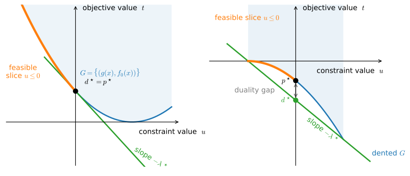
The geometric idea can be sketched without the proof. Map every \(\mathbf{x}\) to the pair \((g(\mathbf{x}), f(\mathbf{x}))\) of constraint value and objective value, and consider the resulting region in the plane (with one constraint, for drawing’s sake). The primal optimum \(p^\star\) is the lowest objective value in the left half-plane \(g \le 0\). Evaluating the dual function at \(\lambda\) amounts to lowering a line of slope \(-\lambda\) until it supports the region from below; its height at \(g = 0\) is \(g(\lambda)\), a lower bound on \(p^\star\): that is weak duality drawn as a picture. For a convex problem the region is convex (more precisely, the set of points above and to the right of it is), so some supporting line passes through the boundary point at \((0, p^\star)\); the granted fact of Section 26.3 supplies a supporting line at a boundary point of a convex set, the same fact that gives convex functions their subgradients. Slater’s strictly feasible point ensures that the region intersects the open left half-plane, ruling out a vertical supporting line, which no finite \(\lambda\) can represent. Then the touching line’s \(\lambda\) achieves \(g(\lambda) = p^\star\): strong duality. For non-convex problems, the boundary can be nonconvex, so every supporting line may pass below the point associated with \(p^\star\), producing a gap; Figure 26.4.3 shows both situations, and we compute an explicit nonconvex example at the end of this section.
Three consequences are useful. First, the dual may be the easier problem: fewer variables, simpler constraints (the SVM dual below has only sign constraints, where the primal couples all margins). Second, the dual certifies: any feasible dual point bounds your suboptimality, which is how solvers know when to stop. Third, when strong duality holds, the KKT conditions Equation 26.4.5 are satisfied by the primal–dual optimal pair, so solving the (convex) dual is solving the primal: recover \(\mathbf{x}^\star\) as the minimizer of \(\mathcal{L}(\cdot, \boldsymbol{\lambda}^\star, \boldsymbol{\nu}^\star)\). One more connection rounds out the toolkit: for linearly constrained problems the dual function is a convex conjugate in disguise. For \(\min f(\mathbf{x})\) s.t. \(A\mathbf{x} \preceq \mathbf{b}\), the Lagrangian is \(f(\mathbf{x}) + \boldsymbol{\lambda}^\top(A\mathbf{x} - \mathbf{b})\), and grouping the terms in \(\mathbf{x}\),
\[ \begin{aligned} g(\boldsymbol{\lambda}) &= \inf_{\mathbf{x}} \left[ f(\mathbf{x}) + (A^\top\boldsymbol{\lambda})^\top\mathbf{x} \right] - \mathbf{b}^\top\boldsymbol{\lambda} \\ &= -\sup_{\mathbf{x}} \left[ (-A^\top\boldsymbol{\lambda})^\top\mathbf{x} - f(\mathbf{x}) \right] - \mathbf{b}^\top\boldsymbol{\lambda} \\ &= -f^*(-A^\top\boldsymbol{\lambda}) - \mathbf{b}^\top\boldsymbol{\lambda}, \end{aligned} \]
with \(f^*\) the conjugate of Section 26.3.5.3. Tables of conjugates are tables of duals.
26.4.4.3 Duality as a Saddle Point
Strong duality has an equivalent formulation that also appears in several modern training objectives. The primal problem can be written in min–max form: for any \(\mathbf{x}\),
\[ \sup_{\boldsymbol{\lambda} \succeq 0,\, \boldsymbol{\nu}} \mathcal{L}(\mathbf{x}, \boldsymbol{\lambda}, \boldsymbol{\nu}) = \begin{cases} f(\mathbf{x}) & \textrm{if } \mathbf{x} \textrm{ is feasible}, \\ +\infty & \textrm{otherwise}, \end{cases} \]
since any violated constraint lets the corresponding multiplier drive the supremum to \(+\infty\), while for feasible \(\mathbf{x}\) the best the multipliers can do is vanish on every slack constraint. So \(p^\star = \inf_{\mathbf{x}} \sup_{\boldsymbol{\lambda} \succeq 0, \boldsymbol{\nu}} \mathcal{L}\) and, by definition, \(d^\star = \sup_{\boldsymbol{\lambda} \succeq 0, \boldsymbol{\nu}} \inf_{\mathbf{x}} \mathcal{L}\): weak duality is the universal inequality \(\sup \inf \le \inf \sup\), and strong duality says that the two optimization orders have equal values. This equality corresponds to a saddle point.
Proposition (strong duality is a saddle point). Suppose strong duality holds for Equation 26.4.3 with both optima attained, at a primal optimum \(\mathbf{x}^\star\) and a dual optimum \((\boldsymbol{\lambda}^\star, \boldsymbol{\nu}^\star)\). Then \((\mathbf{x}^\star, \boldsymbol{\lambda}^\star, \boldsymbol{\nu}^\star)\) is a saddle point of the Lagrangian: for all \(\mathbf{x}\) and all \(\boldsymbol{\lambda} \succeq 0\), \(\boldsymbol{\nu}\),
\[ \mathcal{L}(\mathbf{x}^\star, \boldsymbol{\lambda}, \boldsymbol{\nu}) \;\le\; \mathcal{L}(\mathbf{x}^\star, \boldsymbol{\lambda}^\star, \boldsymbol{\nu}^\star) \;\le\; \mathcal{L}(\mathbf{x}, \boldsymbol{\lambda}^\star, \boldsymbol{\nu}^\star). \tag{26.4.11}\]
Conversely, any saddle point of \(\mathcal{L}\) over \(\mathbf{x} \times (\boldsymbol{\lambda} \succeq 0, \boldsymbol{\nu})\) closes the duality gap, with saddle value \(p^\star = d^\star\).
Proof. Using the definitions and weak duality,
\[ d^\star = g(\boldsymbol{\lambda}^\star, \boldsymbol{\nu}^\star) = \inf_{\mathbf{x}} \mathcal{L}(\mathbf{x}, \boldsymbol{\lambda}^\star, \boldsymbol{\nu}^\star) \;\le\; \mathcal{L}(\mathbf{x}^\star, \boldsymbol{\lambda}^\star, \boldsymbol{\nu}^\star) \;\le\; f(\mathbf{x}^\star) = p^\star, \]
where the last inequality holds because \(\lambda_i^\star \ge 0\) and \(g_i(\mathbf{x}^\star) \le 0\) make every added term nonpositive. Strong duality makes every inequality in this chain an equality. Equality in the first inequality says \(\mathbf{x}^\star\) minimizes \(\mathcal{L}(\cdot, \boldsymbol{\lambda}^\star, \boldsymbol{\nu}^\star)\), the right half of Equation 26.4.11. Equality in the second forces \(\sum_i \lambda_i^\star g_i(\mathbf{x}^\star) = 0\) (complementary slackness, re-derived), whence for any \(\boldsymbol{\lambda} \succeq 0\) and \(\boldsymbol{\nu}\), \(\mathcal{L}(\mathbf{x}^\star, \boldsymbol{\lambda}, \boldsymbol{\nu}) = f(\mathbf{x}^\star) + \sum_i \lambda_i g_i(\mathbf{x}^\star) \le f(\mathbf{x}^\star) = \mathcal{L}(\mathbf{x}^\star, \boldsymbol{\lambda}^\star, \boldsymbol{\nu}^\star)\), the left half. For the converse, a saddle point gives
\[ \inf_{\mathbf{x}} \sup_{\boldsymbol{\lambda} \succeq 0,\, \boldsymbol{\nu}} \mathcal{L} \;\le\; \sup_{\boldsymbol{\lambda} \succeq 0,\, \boldsymbol{\nu}} \mathcal{L}(\mathbf{x}^\star, \boldsymbol{\lambda}, \boldsymbol{\nu}) = \mathcal{L}(\mathbf{x}^\star, \boldsymbol{\lambda}^\star, \boldsymbol{\nu}^\star) = \inf_{\mathbf{x}} \mathcal{L}(\mathbf{x}, \boldsymbol{\lambda}^\star, \boldsymbol{\nu}^\star) \;\le\; \sup_{\boldsymbol{\lambda} \succeq 0,\, \boldsymbol{\nu}} \inf_{\mathbf{x}} \mathcal{L}, \]
i.e. \(p^\star \le d^\star\); weak duality supplies the reverse inequality. \(\blacksquare\)
The saddle-point formulation also describes a family of minimax training objectives. Generative adversarial networks (Section 16.1) and adversarial training are \(\min_{\boldsymbol{\theta}} \max_{\boldsymbol{\phi}}\) problems in the same min–max form (Goodfellow et al. 2014; Madry et al. 2018), and equality between the \(\min\max\) and \(\max\min\) values holds when an appropriate saddle point exists. A duality gap separates these values. This formulation also underlies primal–dual methods, which descend in \(\mathbf{x}\) and ascend in \(\boldsymbol{\lambda}\) simultaneously, converging (for convex problems) to the saddle rather than to a minimum.
26.4.4.4 Sensitivity and Shadow Prices
Optimal multipliers \(\boldsymbol{\lambda}^\star\) quantify sensitivity to constraint perturbations, an interpretation used in economics, operations research, and machine learning. Perturb the constraints: for \(\mathbf{u} \in \mathbb{R}^m\) let
\[ p^\star(\mathbf{u}) = \inf\,\{ f(\mathbf{x}) : g_i(\mathbf{x}) \le u_i,\; h_j(\mathbf{x}) = 0 \}, \]
so \(p^\star(\mathbf{0})\) is our original optimum and \(u_i > 0\) relaxes constraint \(i\).
Proposition (multipliers are shadow prices). Suppose strong duality holds with dual optimum \((\boldsymbol{\lambda}^\star, \boldsymbol{\nu}^\star)\). Then for every \(\mathbf{u}\),
\[ p^\star(\mathbf{u}) \;\ge\; p^\star(\mathbf{0}) - \boldsymbol{\lambda}^{\star\top} \mathbf{u}, \tag{26.4.12}\]
and if \(p^\star(\cdot)\) is differentiable at \(\mathbf{0}\), then \(\lambda_i^\star = -\partial p^\star / \partial u_i\).
Proof. Let \(\mathbf{x}\) be feasible for the perturbed problem: \(g_i(\mathbf{x}) \le u_i\), \(h_j(\mathbf{x}) = 0\). Then
\[ p^\star(\mathbf{0}) = g(\boldsymbol{\lambda}^\star, \boldsymbol{\nu}^\star) \;\le\; f(\mathbf{x}) + \sum_i \lambda_i^\star g_i(\mathbf{x}) + \sum_j \nu_j^\star h_j(\mathbf{x}) \;\le\; f(\mathbf{x}) + \boldsymbol{\lambda}^{\star\top}\mathbf{u}, \]
using strong duality, the definition of \(g\) as an infimum, and \(\lambda_i^\star g_i(\mathbf{x}) \le \lambda_i^\star u_i\). Taking the infimum over all such \(\mathbf{x}\) gives \(p^\star(\mathbf{0}) \le p^\star(\mathbf{u}) + \boldsymbol{\lambda}^{\star\top}\mathbf{u}\), which is Equation 26.4.12. If \(p^\star\) is differentiable at \(\mathbf{0}\), then Equation 26.4.12 says the affine function \(p^\star(\mathbf{0}) - \boldsymbol{\lambda}^{\star\top}\mathbf{u}\) minorizes \(p^\star(\mathbf{u})\) and touches it at \(\mathbf{u} = \mathbf{0}\), so it is the tangent there, and matching gradients gives \(\nabla p^\star(\mathbf{0}) = -\boldsymbol{\lambda}^\star\). \(\blacksquare\)
The multiplier \(\lambda_i^\star\) is the shadow price of constraint \(i\): relaxing the constraint by one unit improves the optimum by approximately \(\lambda_i^\star\). Complementary slackness sets the multiplier of a slack constraint to zero; only binding constraints can have a positive multiplier. In the ball projection, \(\lambda^\star = \|\mathbf{x}_0\|/r - 1\) prices the radius; in the hyperplane example, \(-\nu^\star\) priced the offset \(b\); and in the water-filling problem below, the equality multiplier equals the marginal value of transmit power, as verified below by finite differences.
26.4.4.5 Weight Decay and Norm Constraints
Weight decay (Section 2.7) adds a penalty to the training loss,
\[ \min_{\mathbf{w}}\; L(\mathbf{w}) + \lambda \|\mathbf{w}\|^2 , \]
and the KKT formulation identifies that penalty as the Lagrangian of a norm constraint,
\[ \min_{\mathbf{w}}\; L(\mathbf{w}) \quad \textrm{subject to} \quad \|\mathbf{w}\|^2 \le r^2 . \]
Compare stationarity conditions. The penalized problem asks \(\nabla L(\mathbf{w}) + 2\lambda \mathbf{w} = \mathbf{0}\); the constrained problem’s KKT stationarity, with multiplier \(\lambda \ge 0\) on \(g(\mathbf{w}) = \|\mathbf{w}\|^2 - r^2\), asks \(\nabla L(\mathbf{w}) + 2\lambda \mathbf{w} = \mathbf{0}\): the same equation, with the weight-decay coefficient playing the multiplier’s role. For convex \(L\) the correspondence is exact in both directions: the minimizer \(\mathbf{w}_\lambda\) of the penalized problem is the solution of the constrained problem with budget \(r = \|\mathbf{w}_\lambda\|\) (it is feasible, and KKT sufficiency certifies it), and conversely any active budget \(r > 0\) with attained minimizer has a multiplier \(\lambda^\star(r)\) whose penalized problem returns the same point; this direction uses KKT necessity, which applies because Slater’s condition holds for every \(r > 0\) (\(\mathbf{w} = \mathbf{0}\) is strictly feasible). Sweeping \(\lambda\) and sweeping \(r\) trace the same regularization path, just parameterized differently. The shadow-price proposition gives \(\lambda^\star = -\partial p^\star / \partial (r^2)\), the marginal reduction in loss from an additional unit of squared-norm budget. When the weight budget is slack (the unregularized minimizer already satisfies \(\|\mathbf{w}\| \le r\)), complementary slackness prices it at \(\lambda^\star = 0\).
Two caveats. First, for the non-convex losses of deep networks the correspondence is local and heuristic, not exact: a stationary point of the penalized problem is a KKT point of the matching constrained problem, but without convexity KKT points need not be global minima and the two problems’ solution sets need not coincide; the same gap that separates \(p^\star\) from \(d^\star\) in the example below can separate the two formulations. Second, the same number has a third, statistical reading: Section 27.3 derives the penalty \(\lambda\|\mathbf{w}\|^2\) as the log of a Gaussian prior (MAP estimation). Thus \(\lambda\) can be interpreted as a Lagrange multiplier, a regularization coefficient, or a parameter of a prior distribution. The cell below verifies the equivalence numerically on ridge regression (\(L(\mathbf{w}) = \|A\mathbf{w} - \mathbf{b}\|^2\), convex, so the theorem applies in full): for each \(\lambda\) it solves the penalized problem in closed form, uses the resulting norm as the constrained problem’s budget \(r\), solves that by projected gradient descent onto the \(r\)-ball, and recovers the multiplier from the KKT stationarity residual:
rng = np.random.default_rng(3)
A, b = rng.normal(size=(30, 5)), rng.normal(size=30)
grad = lambda w: 2 * A.T @ (A @ w - b)           # gradient of L = |Aw - b|^2
step = 1.0 / (2 * np.linalg.eigvalsh(A.T @ A).max())
print(' lambda    r = |w_pen|   |w_con - w_pen|   recovered multiplier')
for lam in [0.1, 1.0, 10.0]:
    w_pen = np.linalg.solve(A.T @ A + lam * np.eye(5), A.T @ b)  # penalty form
    r = np.linalg.norm(w_pen)                    # its norm becomes the budget
    w = np.zeros(5)                              # constraint form: PGD, radius r
    for _ in range(5000):
        w -= step * grad(w)
        w *= min(1.0, r / np.linalg.norm(w))     # project onto the r-ball
    lam_rec = -(w @ grad(w)) / (2 * r * r)       # KKT: grad L + 2*lam*w = 0
    print(f'{lam:7.2f}  {r:11.4f}  {np.linalg.norm(w - w_pen):15.2e}  '
          f'{lam_rec:17.4f}')
lambda r = |w_pen| |w_con - w_pen| recovered multiplier
0.10 0.4460 9.23e-17 0.1000
1.00 0.4235 9.64e-17 1.0000
10.00 0.2840 5.55e-17 10.0000Three different decay strengths, and in every row the constrained solution matches the penalized one to \(10^{-16}\) while the multiplier recovered from the constrained problem’s own KKT residual reproduces \(\lambda\) to four decimals. Penalty and constraint give two parameterizations of the same convex solution family, and the multiplier connects them.
26.4.5 Worked Duals: SVM, Water-Filling, and an Explicit Gap
26.4.5.1 The Support Vector Machine Dual
The support-vector machine (Cortes and Vapnik 1995) is a standard example in which the dual exposes useful structure. Given linearly separable data \((\mathbf{x}_i, y_i)\) with labels \(y_i \in \{\pm 1\}\), the maximum-margin separating hyperplane \(\mathbf{w}^\top\mathbf{x} + b = 0\) solves
\[ \min_{\mathbf{w}, b}\; \tfrac12 \|\mathbf{w}\|^2 \quad \textrm{subject to} \quad y_i\,(\mathbf{w}^\top \mathbf{x}_i + b) \ge 1, \;\; i = 1, \ldots, n, \tag{26.4.13}\]
since, by the signed-distance formula of Section 24.1 (a point \(\mathbf{x}\) lies at distance \(|\mathbf{w}^\top\mathbf{x} + b| / \|\mathbf{w}\|\) from the hyperplane), the two margin hyperplanes \(\mathbf{w}^\top\mathbf{x} + b = \pm 1\) sit at distance \(1/\|\mathbf{w}\|\) on either side of the boundary, \(2/\|\mathbf{w}\|\) apart: minimizing \(\|\mathbf{w}\|\) is maximizing the margin. This is a convex QP with one inequality per data point; Slater holds for strictly separable data (scale any separating \((\mathbf{w}, b)\) up until all margins exceed \(1\)), so strong duality is guaranteed. Form the Lagrangian with multipliers \(\alpha_i \ge 0\),
\[ \mathcal{L}(\mathbf{w}, b, \boldsymbol{\alpha}) = \tfrac12\|\mathbf{w}\|^2 + \sum_i \alpha_i \left(1 - y_i(\mathbf{w}^\top\mathbf{x}_i + b)\right), \]
and compute the dual function \(g(\boldsymbol{\alpha}) = \inf_{\mathbf{w}, b} \mathcal{L}\). The Lagrangian is affine in \(b\), with coefficient \(-\sum_i \alpha_i y_i\): unless that coefficient vanishes, sending \(b\) to \(\pm\infty\) drives \(\mathcal{L}\) to \(-\infty\), so \(g(\boldsymbol{\alpha}) = -\infty\) whenever \(\sum_i \alpha_i y_i \neq 0\). This is the effective-domain mechanism promised at Equation 26.4.9: multipliers with \(\sum_i \alpha_i y_i \neq 0\) lie outside the dual function’s effective domain, so the vanishing condition reappears as the dual’s equality constraint. On that domain the \(b\)-term drops out of \(\mathcal{L}\) entirely, leaving a strictly convex quadratic in \(\mathbf{w}\) whose infimum is attained at its stationary point,
\[ \mathbf{w} = \sum_i \alpha_i y_i\, \mathbf{x}_i, \qquad\textrm{on the domain}\qquad \sum_i \alpha_i y_i = 0. \]
The weight vector is a combination of the data, with coefficients the multipliers. Substituting back yields the SVM dual:
\[ \max_{\boldsymbol{\alpha} \succeq 0,\ \sum_i \alpha_i y_i = 0}\;\; \sum_i \alpha_i \;-\; \tfrac12 \sum_{i,j} \alpha_i \alpha_j\, y_i y_j\, \mathbf{x}_i^\top \mathbf{x}_j. \tag{26.4.14}\]
Two consequences hold before any algorithm is chosen. Complementary slackness, \(\alpha_i (1 - y_i(\mathbf{w}^\top\mathbf{x}_i + b)) = 0\), says \(\alpha_i > 0\) only for points exactly on the margin: the support vectors, the active constraints of the active-set picture in Figure 26.4.2. All other points have \(\alpha_i = 0\) and do not contribute to the recovered weight vector. And the data enter Equation 26.4.14 only through inner products \(\mathbf{x}_i^\top\mathbf{x}_j\): replace them by a kernel evaluation \(k(\mathbf{x}_i, \mathbf{x}_j)\) and the resulting dual defines a nonlinear classifier, an option the primal formulation does not expose.
We can solve the dual using the preceding conditions. One simplification first: the equality constraint \(\sum_i \alpha_i y_i = 0\) entered only because the unpenalized offset \(b\) made the Lagrangian affine in one direction. If we instead fold the offset into the weights (append a constant feature, \(\tilde{\mathbf{x}}_i = (\mathbf{x}_i, 1)\) and \(\tilde{\mathbf{w}} = (\mathbf{w}, b)\), so the primal becomes \(\min \tfrac12\|\tilde{\mathbf{w}}\|^2\) subject to \(y_i \tilde{\mathbf{w}}^\top \tilde{\mathbf{x}}_i \ge 1\)), then the Lagrangian is strictly convex in every primal variable, its infimum is finite for every \(\boldsymbol{\alpha}\), the equality constraint never appears, and the dual feasible set is the plain nonnegative orthant \(\boldsymbol{\alpha} \succeq 0\), on which projection is a coordinate-wise clip. (One caveat in labeling: this variant also regularizes the offset, so its maximum-margin boundary can differ slightly from Equation 26.4.13’s; the duality structure is identical.) Writing \(Q_{ij} = y_i y_j \tilde{\mathbf{x}}_i^\top \tilde{\mathbf{x}}_j\), the dual is
\[ \max_{\boldsymbol{\alpha} \succeq 0}\;\; \mathbf{1}^\top \boldsymbol{\alpha} - \tfrac12 \boldsymbol{\alpha}^\top Q\, \boldsymbol{\alpha}, \]
a concave quadratic over the orthant, exactly the setting of Equation 26.4.7. Projected gradient ascent iterates \(\boldsymbol{\alpha} \leftarrow \max(\mathbf{0},\, \boldsymbol{\alpha} + \eta\,(\mathbf{1} - Q\boldsymbol{\alpha}))\) with \(\eta = 1/\lambda_{\max}(Q)\), the dual’s own descent-lemma step size. The cell below runs it on a small 2-D toy problem and then checks this section’s claims: the recovered \((\mathbf{w}^\star, b^\star)\) separates the data, complementary slackness holds to machine precision, and the dual value meets the primal value: strong duality, observed.
X = np.array([[1.0, 1.5], [2.0, 0.5], [2.5, 2.0], [1.5, 3.0],
              [-1.0, -0.5], [-2.0, 1.0], [-1.5, -2.0], [0.5, -1.5]])
y_pm = np.array([1.0, 1.0, 1.0, 1.0, -1.0, -1.0, -1.0, -1.0])
Xa = np.hstack([X, np.ones((len(X), 1))])     # fold the offset b into w
G = y_pm[:, None] * Xa
Q = G @ G.T                                   # Q_ij = y_i y_j x_i^T x_j
alpha = np.zeros(len(X))
eta = 1.0 / np.linalg.eigvalsh(Q).max()       # 1/L for the dual objective
for _ in range(5000):                         # projected gradient ascent
    alpha = np.maximum(0.0, alpha + eta * (1.0 - Q @ alpha))
w = G.T @ alpha                               # w* = sum_i alpha_i y_i x_i
margins = y_pm * (Xa @ w)
dual = alpha.sum() - 0.5 * alpha @ Q @ alpha
primal = 0.5 * w @ w
print('alpha* =', alpha.round(4))
print('w* =', w[:2].round(4), ' b* =', w[2].round(4),
      ' separates data:', bool((np.sign(Xa @ w) == y_pm).all()))
print('margins y_i (w^T x_i + b) =', margins.round(4))
print('KKT: comp. slack', f'{np.abs(alpha * (margins - 1.0)).max():.1e}',
      '| worst primal feas.', f'{(1.0 - margins).max():.1e}')
print(f'primal = {primal:.6f}, dual = {dual:.6f}, gap = {abs(primal - dual):.1e}')
alpha* = [0.1309 0.0732 0. 0. 0. 0.2442 0. 0.3885]
w* = [0.5714 0.5714] b* = -0.4286 separates data: True
margins y_i (w^T x_i + b) = [1. 1. 2.1429 2.1429 1.2857 1. 2.4286 1. ]
KKT: comp. slack 3.0e-16 | worst primal feas. 7.8e-16
primal = 0.418367, dual = 0.418367, gap = 4.4e-16The printout illustrates these properties. Four of the eight multipliers are strictly positive, and exactly those four points have margin \(1.0000\): the support vectors, whose margin equality follows from complementary slackness; the other four points sit at margins \(1.29\)–\(2.43\) with \(\alpha_i = 0\). The solution is exact enough to recognize: \(\mathbf{w}^\star = (\tfrac47, \tfrac47)\), \(b^\star = -\tfrac37\), with \(p^\star = d^\star = \tfrac{41}{98} \approx 0.418367\) and a primal–dual gap at \(10^{-16}\) after five thousand fixed-step projected-ascent iterations. The primal–dual gap therefore certifies optimality to machine precision. The printout also verifies an identity derived in Exercise 6: \(\sum_i \alpha_i^\star = \|\tilde{\mathbf{w}}^\star\|^2\) at the optimum, which is why the dual and primal values coincide line for line.
26.4.5.2 Water-Filling
The second dual has a closed-form solution with a standard geometric interpretation. A transmitter splits a power budget \(P\) across \(n\) independent channels; channel \(i\) has noise level \(n_i > 0\), and the achievable communication rate is \(\sum_i \log(1 + p_i / n_i)\) (Cover and Thomas 1999). The allocation problem,
\[ \max_{\mathbf{p}}\; \sum_{i=1}^n \log\left(1 + \frac{p_i}{n_i}\right) \quad \textrm{subject to} \quad \mathbf{p} \succeq 0, \;\; \sum_i p_i = P, \tag{26.4.15}\]
is convex (concave objective, affine constraints) with Slater trivially satisfied, so the KKT conditions characterize the global optimum. With multiplier \(\mu\) for the budget and \(\lambda_i \ge 0\) for \(p_i \ge 0\), stationarity reads
\[ \frac{1}{n_i + p_i} = \mu - \lambda_i. \]
On channels with \(p_i > 0\), complementary slackness sets \(\lambda_i\) to zero and forces \(n_i + p_i = 1/\mu\): the same constant for every active channel. On dry channels, \(p_i = 0\) requires \(\lambda_i = \mu - 1/n_i \ge 0\), i.e. \(n_i \ge 1/\mu\). Writing \(w = 1/\mu\) for that constant:
\[ p_i^\star = \max(w - n_i,\, 0), \qquad \textrm{with } w \textrm{ set by } \sum_i \max(w - n_i,\, 0) = P. \]
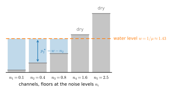
This is the water-filling solution: represent each channel as a basin with floor height \(n_i\) and allocate \(P\) units of water. As Figure 26.4.4 shows, the water settles at a common level \(w\), filling the deep (quiet) channels most, and never reaching basins whose floor is above the waterline. The level is the unique root of a continuous, nondecreasing, piecewise-linear function of \(w\), so bisection finds it. The threshold structure is the same KKT case split as the simplex projection’s \(\tau\), with a different objective.
The shadow-price proposition gives the multiplier its engineering meaning: \(\mu^\star = 1/w\) is the derivative of the optimal rate with respect to the power budget, which the cell checks by re-solving at \(P \pm 10^{-4}\).
noise = np.array([0.1, 0.4, 0.8, 1.6, 2.5])   # channel noise floors
P = 3.0                                       # total power budget

def water_fill(P, noise, steps=60):
    lo, hi = noise.min(), noise.min() + P     # bracket for the water level
    for _ in range(steps):                    # bisection on the level
        mid = 0.5 * (lo + hi)
        lo, hi = (mid, hi) if np.maximum(0, mid - noise).sum() < P else (lo, mid)
    level = 0.5 * (lo + hi)
    return level, np.maximum(0.0, level - noise)

level, p = water_fill(P, noise)
print('water level w =', f'{level:.6f}', ' p* =', p.round(4),
      ' total =', f'{p.sum():.6f}')
print('wet channels filled to common level:', (noise + p)[p > 0].round(6))
print('dry channels above the waterline:   ', bool((noise[p == 0] >= level).all()))
rate = lambda q: np.log(1.0 + q / noise).sum()
dP = 1e-4                                     # shadow price, two ways
mu = 1.0 / level
sens = (rate(water_fill(P + dP, noise)[1])
        - rate(water_fill(P - dP, noise)[1])) / (2 * dP)
print(f'mu = 1/w = {mu:.6f} vs finite-difference dU*/dP = {sens:.6f}')
water level w = 1.433333 p* = [1.3333 1.0333 0.6333 0. 0. ] total = 3.000000
wet channels filled to common level: [1.433333 1.433333 1.433333]
dry channels above the waterline: True
mu = 1/w = 0.697674 vs finite-difference dU*/dP = 0.697674The budget is met to ten digits, the three wet channels are filled to the identical level \(w = 1.4333\), the two channels with floors \(1.6\) and \(2.5\) stay dry exactly as dual feasibility demands, and the multiplier \(\mu = 1/w = 0.6977\) matches the finite-difference sensitivity of the optimal rate to the budget through six digits. Perturbing the constraint verifies this shadow-price interpretation.
26.4.5.3 An Explicit Duality Gap
Weak duality always holds, whereas strong duality need not. The following one-dimensional problem gives an explicit counterexample: on the interval \(x \in [0, 1]\),
\[ \min_x\; f_0(x) = -x^2 \quad \textrm{subject to} \quad f_1(x) = x - \tfrac12 \le 0. \]
The objective is concave (this is a non-convex problem) and the feasible region is \([0, \tfrac12]\), so the primal optimum is at the boundary: \(p^\star = f_0(\tfrac12) = -\tfrac14\). The dual function is computable by hand: \(\mathcal{L}(x, \lambda) = -x^2 + \lambda(x - \tfrac12)\) is concave in \(x\), so its minimum over \([0, 1]\) is at an endpoint, giving \(g(\lambda) = \min(-\lambda/2,\; \lambda/2 - 1)\): piecewise linear, concave (as it must be), and maximized at \(\lambda = 1\) with \(d^\star = -\tfrac12 < -\tfrac14 = p^\star\): a duality gap of exactly \(\tfrac14\). The cell verifies all of it numerically and plots the maximum of the dual function strictly below \(p^\star\).
xs = np.linspace(0.0, 1.0, 4001)              # the domain D = [0, 1]
f0, f1 = -xs**2, xs - 0.5                     # objective and constraint
p_star = f0[f1 <= 0.0].min()                  # primal optimum: -1/4
lams = np.linspace(0.0, 3.0, 601)
g = np.array([(f0 + lam * f1).min() for lam in lams])  # dual function
d_star, lam_star = g.max(), lams[g.argmax()]
print(f'p* = {p_star:.4f},  d* = {d_star:.4f} at lambda = {lam_star:.2f},'
      f'  gap = {p_star - d_star:.4f}')
print('weak duality g(lambda) <= p* everywhere:',
      bool((g <= p_star + 1e-12).all()))
d2l.plot(lams, [g, np.full_like(lams, p_star)], 'lambda', 'value',
legend=['dual function g(lambda)', 'primal optimum p*'])p* = -0.2500, d* = -0.5000 at lambda = 1.00, gap = 0.2500
weak duality g(lambda) <= p* everywhere: True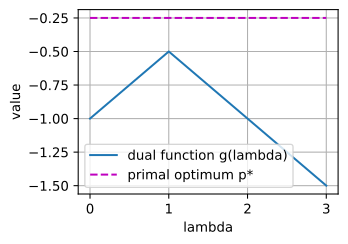
p* = -0.2500,  d* = -0.5000 at lambda = 1.00,  gap = 0.2500
weak duality g(lambda) <= p* everywhere: True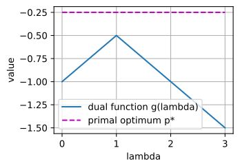
p* = -0.2500,  d* = -0.5000 at lambda = 1.00,  gap = 0.2500
weak duality g(lambda) <= p* everywhere: True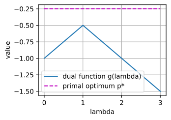
p* = -0.2500,  d* = -0.5000 at lambda = 1.00,  gap = 0.2500
weak duality g(lambda) <= p* everywhere: True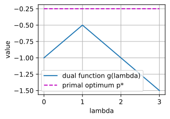
This example also shows that a strictly feasible point can exist (\(x = 0\) has \(f_1 = -\tfrac12 < 0\)), yet the gap is real: Slater’s condition certifies strong duality only for convex problems, and \(f_0 = -x^2\) is not convex. In the supporting-line picture of Figure 26.4.3, the nonconvex curve \(\{(f_1(x), f_0(x))\} = \{(u, -(u + \tfrac12)^2)\}\) admits no supporting line through its point at \(u = 0\), and the best available line (slope \(-1\), our \(\lambda^\star = 1\)) certifies only \(-\tfrac12\). For non-convex training problems, duals still give valid lower bounds (and are the engine of verification and relaxation methods), but the bound need not be tight.
26.4.5.4 Convexity and Duality Across Problem Classes
The examples above were all quadratic programs, but they sit inside a standard hierarchy of convex problem classes (Boyd and Vandenberghe 2004); each class corresponds to standard solver families:
| Class | Template | Machine-learning examples |
|---|---|---|
| LP (linear program) | linear \(f\), constraints \(A\mathbf{x} \preceq \mathbf{b}\) | \(\ell_1\) / \(\ell_\infty\) reformulations, optimal transport |
| QP (quadratic program) | convex quadratic \(f\), affine constraints | ridge, lasso, SVM dual, simplex projection, trust-region step |
| SOCP (second-order cone program) | cones \(\|A\mathbf{x} + \mathbf{b}\| \le \mathbf{c}^\top\mathbf{x} + d\) | max-norm weight constraints, robust losses |
| SDP (semidefinite program) | matrix variable \(X \succeq 0\), the semidefinite sense of \(\succeq\) (Section 26.3) | spectral-norm bounds, nuclear-norm relaxations |
Each class contains the previous (\(\mathrm{LP} \subseteq \mathrm{QP} \subseteq \mathrm{SOCP} \subseteq \mathrm{SDP}\)), and all are solvable to high accuracy in polynomial time by interior-point methods, which replace the constraints by a barrier and follow the smoothed problems’ solutions to the boundary (Boyd and Vandenberghe 2004; Nesterov 2018; Nocedal and Wright 2006). Training a deep network lies outside the hierarchy, since the composition of layers destroys convexity (Section 26.3); but many of its sub-problems are convex, where multipliers, KKT, and duality apply directly: projections, clipped updates, last-layer fits, and the trust-region step, which minimizes a local quadratic model of the objective within a ball around the current iterate (Nocedal and Wright 2006).
26.4.6 Summary
- A constrained optimum is a point with no feasible descent direction. For one equality constraint with \(\nabla g(\mathbf{x}^\star) \neq \mathbf{0}\) this forces \(\nabla f = -\nu \nabla g\); the Lagrangian \(\mathcal{L} = f + \nu g\) packages the condition and the constraint as joint stationarity.
- With inequalities, the KKT conditions govern: stationarity, primal and dual feasibility (\(\lambda_i \ge 0\)), and complementary slackness \(\lambda_i g_i = 0\), which finds the active set. KKT is necessary under a constraint qualification and sufficient for global optimality in convex problems.
- Projections onto nonempty closed convex sets are unique and nonexpansive. For convex \(L\)-smooth objectives, projected gradient descent with a suitable step has the usual \(O(1/k)\) value guarantee. Its fixed points satisfy constrained first-order stationarity; convexity of the objective is what upgrades stationarity to global optimality. The simplex projection is a KKT-derived sort-and-threshold (sparsemax).
- The dual function \(g(\boldsymbol{\lambda}, \boldsymbol{\nu}) = \inf_{\mathbf{x}} \mathcal{L}\) is always concave, and weak duality \(d^\star \le p^\star\) always holds: dual points are certificates. Slater’s condition (convexity plus a strictly feasible point) closes the gap; without convexity a gap can survive even with strictly feasible points.
- Strong duality is the same statement as a saddle point of the Lagrangian (\(\inf \sup = \sup \inf\)), which provides the basis for primal–dual methods and minimax objectives such as GANs and adversarial training. Weight decay is the central application: the penalty \(\lambda\|\mathbf{w}\|^2\) and the constraint \(\|\mathbf{w}\|^2 \le r^2\) share one KKT stationarity equation. Under convexity and suitable regularity, an active constraint and its optimal multiplier connect corresponding solutions; inactive constraints, zero multipliers, and nonunique solutions prevent a one-to-one correspondence. For deep networks the analogy is local and heuristic.
- Multipliers are shadow prices: \(\lambda_i^\star = -\partial p^\star/\partial u_i\) measures what relaxing constraint \(i\) is worth. It is \(1/w\) in water-filling, and it is why slack constraints have zero shadow price.
- The SVM dual (support vectors = active constraints, kernels via inner products) and water-filling (pour to a common level, bisection on the level) show the full pipeline; LP/QP/SOCP/SDP is the solver map for the convex sub-problems of deep learning.
26.4.7 Exercises
- Derive the Lagrange condition for two equality constraints: if \(\mathbf{x}^\star\) is a local minimum of \(f\) on \(\{h_1 = 0\} \cap \{h_2 = 0\}\) and \(\nabla h_1(\mathbf{x}^\star)\), \(\nabla h_2(\mathbf{x}^\star)\) are linearly independent, show \(\nabla f(\mathbf{x}^\star) \in \mathrm{span}\{\nabla h_1, \nabla h_2\}\) by the no-feasible-descent argument. Then revisit the counterexample (\(\min x_1\) s.t. \(x_1^2 + x_2^2 = 0\)) and identify exactly which step of your proof fails there.
- Maximize the entropy \(-\sum_i p_i \log p_i\) over the probability simplex using one multiplier for \(\sum_i p_i = 1\), and show the optimum is the uniform distribution. Where did you use that the \(p_i > 0\) constraints are inactive at the optimum? (Compare Section 26.3.3, which reaches the same conclusion through Jensen’s inequality.)
- Write all four KKT conditions for \(\min\, \tfrac12\|\mathbf{x} - \mathbf{x}_0\|^2\) s.t. \(\|\mathbf{x}\|^2 \le r^2\) and verify the clipping solution and \(\lambda^\star = \max(0, \|\mathbf{x}_0\|/r - 1)\). Then exhibit a one-dimensional non-convex problem with a KKT point that is a local maximum: necessity without sufficiency.
- Show that \(\mathbf{x}^\star\) is a fixed point of the projected gradient update Equation 26.4.7 with \(C = \{\mathbf{x} : \mathbf{x} \succeq 0\}\) if and only if for each coordinate either \(\partial f/\partial x_i = 0\) and \(x_i^\star \ge 0\), or \(\partial f/\partial x_i > 0\) and \(x_i^\star = 0\); then check this is precisely KKT for the constraints \(-x_i \le 0\).
- Prove from the definitions that the dual function of any primal problem is concave, and that weak duality holds (reproduce the proofs without looking). Then compute the dual of the equality-constrained QP \(\min\, \tfrac12\mathbf{x}^\top A \mathbf{x} - \mathbf{b}^\top\mathbf{x}\) s.t. \(C\mathbf{x} = \mathbf{d}\) with \(A \succ 0\) in closed form, and verify \(d^\star = p^\star\) by solving both sides for \(A = \mathrm{diag}(1, 2)\), \(\mathbf{b} = (1, 1)\), \(C = (1\;\; 1)\), \(d = 1\).
- For the offset-folded SVM dual \(\max_{\boldsymbol{\alpha} \succeq 0} \mathbf{1}^\top\boldsymbol{\alpha} - \tfrac12 \boldsymbol{\alpha}^\top Q \boldsymbol{\alpha}\), show that at the optimum \(\sum_i \alpha_i^\star = \|\tilde{\mathbf{w}}^\star\|^2\) where \(\tilde{\mathbf{w}}^\star = \sum_i \alpha_i^\star y_i \tilde{\mathbf{x}}_i\). (Hint: multiply the KKT stationarity condition \((\mathbf{1} - Q\boldsymbol{\alpha}^\star)_i = -\lambda_i^\star \le 0\) by \(\alpha_i^\star\), sum, and use complementary slackness.) Conclude that the dual optimal value equals \(\tfrac12\|\tilde{\mathbf{w}}^\star\|^2\), as the
#constrained-svm-dualcell observed numerically. - In water-filling Equation 26.4.15, show that the optimal rate \(U^\star(P)\) is concave and piecewise smooth in \(P\), that the water level \(w(P)\) is piecewise linear and increasing, and that the shadow price \(\mu = 1/w\) therefore decreases with the budget: diminishing returns. At which values of \(P\) (for the noise floors in the
#constrained-water-fillingcell) does the slope change, and why? - Rerun the duality-gap demo with the objective \(f_0(x) = +x^2\) in place of \(-x^2\) (everything else unchanged). Compute \(p^\star\) and \(d^\star\) by hand and numerically, and explain in terms of Slater’s condition why the gap is now zero.
26.4.8 Discussions
These methods connect directly to applications in the main book. The penalty form of regularization (add \(\lambda\|\mathbf{w}\|^2\) to the loss) and the constraint form (minimize the loss subject to \(\|\mathbf{w}\|^2 \le r^2\)) are linked precisely by the Lagrangian: the weight-decay coefficient of Section 2.7 is the multiplier of the norm constraint, and sweeping one traces out the solutions of the other. Projections support gradient clipping and constrained updates, and the simplex projection is sparsemax. Within this part, the section leans on Section 26.3 (convexity, the conjugate) and Section 26.1 (descent lemma, rates), and its conditioning consequences continue in Section 26.5.