%matplotlib inline
from d2l import torch as d2l
import numpy as np
import torch
import torchvision
d2l.use_svg_display()27.7 Naive Bayes
The naive Bayes classifier estimates a probabilistic model from counts and predicts with Bayes’ rule. Its conditional-independence assumption reduces a high-dimensional density estimate to separate estimates for each feature. This section derives the classifier, applies it to handwritten digits, and evaluates its errors and calibration. A bootstrap interval quantifies uncertainty in its accuracy.
%matplotlib inline
from d2l import tensorflow as d2l
import numpy as np
import tensorflow as tf
d2l.use_svg_display()%matplotlib inline
from d2l import jax as d2l
import numpy as np
import tensorflow as tf
d2l.use_svg_display()%matplotlib inline
from d2l import mxnet as d2l
from mxnet import gluon, npx
from mxnet import np as mnp
import numpy as np
npx.set_np()
d2l.use_svg_display()27.7.1 Bayes’ Rule for Classification
A classifier maps an example \(\mathbf{x}\in\mathbb{R}^d\) to a label \(y\in\{1,\ldots,K\}\). A probabilistic classifier estimates the posterior \(p(y\mid\mathbf{x})\) and predicts its most probable label:
\[\hat{y} = \mathop{\mathrm{argmax}}_y \, p(y\mid\mathbf{x}). \tag{27.7.1}\]
An unconstrained table for \(p(y\mid\mathbf{x})\) is impractical in high dimensions. With \(d\) binary features there are \(2^d\) possible inputs, so the table grows exponentially and most entries receive little or no data. For an MNIST image, \(d=784\).
Bayes’ rule Equation 27.1.16 expresses this posterior in terms of a class-conditional distribution, the generative direction:
\[\hat{y} = \mathop{\mathrm{argmax}}_y \, p(y\mid\mathbf{x}) = \mathop{\mathrm{argmax}}_y \, \frac{p(\mathbf{x}\mid y)\,p(y)}{p(\mathbf{x})} = \mathop{\mathrm{argmax}}_y \, p(\mathbf{x}\mid y)\,p(y). \tag{27.7.2}\]
The denominator \(p(\mathbf{x})\) is independent of \(y\) and therefore does not affect the maximizing label. Hence \(p(y\mid\mathbf{x})\propto p(\mathbf{x}\mid y)p(y)\). If normalized posterior probabilities are needed, divide these class scores by their sum.
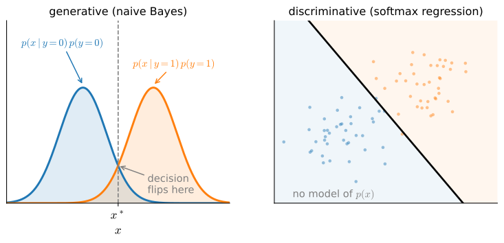
A generative classifier models the class-conditional distribution \(p(\mathbf{x}\mid y)\) and the prior \(p(y)\), then applies Bayes’ rule. A discriminative classifier, such as logistic regression or the softmax classifier in Section 3.1, models \(p(y\mid\mathbf{x})\) directly and need not specify the input distribution.
For the models studied by Ng and Jordan (2002), a generative classifier can approach its asymptotic error with fewer examples, while a discriminative model can attain a lower asymptotic error. This comparison depends on the model and data distribution; neither ordering is universal. Naive Bayes is a simple generative classifier. Figure 27.7.1 compares the two approaches.
This reformulation alone does not reduce the number of parameters: \(p(\mathbf{x}\mid y)\) is still a distribution over \(2^d\) binary patterns. The probability chain rule (Section 27.1) gives
\[p(\mathbf{x}\mid y) = p(x_1\mid y)\,p(x_2\mid x_1, y)\cdots p(x_d\mid x_1,\ldots,x_{d-1}, y), \tag{27.7.3}\]
The later factors depend on increasingly long feature histories, so the unrestricted model still requires exponentially many parameters.
27.7.1.1 The Naive Assumption
Naive Bayes assumes that the features are jointly conditionally independent given the label. Pairwise conditional independence is insufficient when \(d>2\); the required assumption factorizes the complete conditional distribution into one-feature marginals:
\[p(\mathbf{x}\mid y) = \prod_{i=1}^d p(x_i\mid y). \tag{27.7.4}\]
For binary features, an unrestricted class-conditional distribution has \(2^d-1\) free probabilities per class. The factorization uses only \(d\) Bernoulli parameters per class, plus \(K-1\) class-prior parameters. This is the computational and statistical benefit of the assumption.
As a graphical model the factorization is a star: the label \(y\) is a parent of each feature, with no edges among features (Figure 27.7.2, left). Pixel data retain substantial conditional dependence after the digit label is known, as illustrated by the additional feature edges in the right panel.
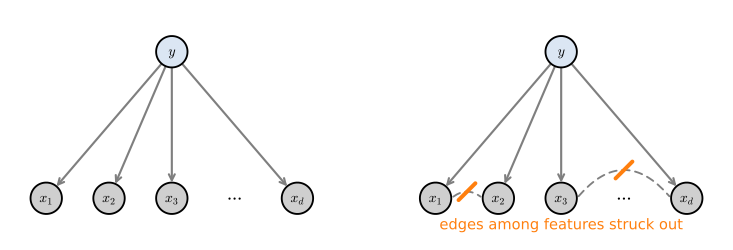
For MNIST this assumption is inaccurate: neighboring pixels remain correlated within a digit class. Nevertheless, classification depends on the ordering of class scores, not on every estimated probability being accurate. Naive Bayes can therefore classify well even when its posterior probabilities are poorly calibrated (Domingos and Pazzani 1997).
Substituting Equation 27.7.4 into the Bayes classifier gives the naive Bayes rule (Maron 1961):
\[\hat{y} = \mathop{\mathrm{argmax}}_y \; p(y) \prod_{i=1}^d p(x_i\mid y). \tag{27.7.5}\]
27.7.1.2 Computation in Log Space
Equation Equation 27.7.5 multiplies \(d\) numbers in \([0,1]\). For \(d=784\), these products can be extremely small. In the MNIST experiment below, 99.1% of the single-precision class scores underflow to zero. Even in float64, the nonzero products range from about \(10^{-26}\) to \(10^{-323}\).
The logarithm is strictly increasing, so it preserves the maximizing class and turns products into sums. Applying it to Equation 27.7.5 yields the stable log-space rule discussed in Section 26.5:
\[\hat{y} = \mathop{\mathrm{argmax}}_y \; \log p(y) + \sum_{i=1}^d \log p(x_i\mid y). \tag{27.7.6}\]
Each class score is now a sum of 785 finite log probabilities rather than a product prone to underflow. Prediction requires a table of precomputed log probabilities and a sequence of additions.
For a binary feature, \(\log p(x_i\mid y)=x_i\log p(x_i=1\mid y)+(1-x_i)\log p(x_i=0\mid y)\). Therefore Equation 27.7.6 becomes
\[\log p(y) + \sum_{i=1}^d \Bigl[ x_i \log p(x_i{=}1\mid y) + (1-x_i)\log p(x_i{=}0\mid y) \Bigr],\]
which is affine in \(\mathbf{x}\), a constant plus a weighted sum of the pixels (Bishop 2006). Thus Bernoulli naive Bayes has class scores \(\mathbf{w}_y\cdot\mathbf{x}+b_y\), and every pairwise decision boundary is a hyperplane. Multinomial naive Bayes is similarly affine in feature counts. These models have the same boundary form as softmax regression, although their parameters are estimated from class-conditional counts rather than by directly optimizing conditional likelihood.
This linear-boundary conclusion does not hold for every naive Bayes likelihood. With Gaussian features, the class score contains \(-(x_i-\mu_{iy})^2/(2\sigma_{iy}^2)\). If the variance of feature \(i\) is shared across classes, its \(x_i^2\) term cancels when two class scores are compared and the boundary is linear. With class-specific variances, the quadratic terms do not cancel, and the boundary is generally quadratic.
27.7.2 Parameter Estimation from Counts
Naive Bayes estimates the class prior \(p(y)\) and the feature likelihoods \(p(x_i\mid y)\). For the categorical and Bernoulli models considered here, their maximum-likelihood estimates are empirical frequencies.
If class \(y\) occurs \(n_y\) times among \(n=\sum_y n_y\) examples, then \(\hat p(y)=n_y/n\). For a binary feature, \(\hat p(x_i=1\mid y)\) is the fraction of class-\(y\) examples in which feature \(i\) is one. We store these values in an array \(P_{xy}\), represented below as one \(28\times28\) grid per class. The complementary probability is \(\hat p(x_i=0\mid y)=1-\hat p(x_i=1\mid y)\).
One hazard remains. If feature \(i\) is never on for class \(y\) in the training set, the MLE is \(\hat p(x_i=1\mid y)=0\), and a single such feature at test time annihilates the whole product in Equation 27.7.5 (and sends Equation 27.7.6 to \(-\infty\)). The cure is Laplace smoothing (Laplace 1814): add a pseudocount, estimating \(p(x_i=1\mid y)\) as \((n_{iy}+1)/(n_y+2)\) rather than \(n_{iy}/n_y\), where \(n_{iy}\) counts the class-\(y\) examples with feature \(i\) on and the \(+2\) covers the two outcomes a binary pixel can take; a categorical feature with \(v\) possible values gets \(+1\) on each value’s count and \(+v\) in the denominator, so the smoothed probabilities still sum to one (the text models at the end of this section smooth the same way, with \(+|V|\) for a vocabulary \(V\)). The pseudocount has a Bayesian justification: \((n_{iy}+1)/(n_y+2)\) is the posterior mean of the Bernoulli parameter under a uniform \(\mathrm{Beta}(1,1)\) prior, Laplace’s rule of succession, as Section 27.3.4.2 derives (along with the numerically coincident, but conceptually distinct, \(\mathrm{Beta}(2,2)\) MAP estimate it is often conflated with).
For continuous features, Gaussian naive Bayes models each feature within each class by a univariate Gaussian (Section 27.2). Training estimates a mean and variance for each class–feature pair, and the log-space score sums Gaussian log densities. In the experiment below we instead threshold pixel intensities into binary features. This produces a simpler model but discards grayscale information.
27.7.3 A Worked Example: MNIST Digits
MNIST contains \(28\times28\) grayscale images of handwritten digits (LeCun et al. 1998). We threshold each pixel at half intensity, so \(x_i\in\{0,1\}\) records whether it is active. The training and test splits are converted to NumPy arrays: X has shape (n, 28, 28) and Y contains integer labels. Subsequent estimation uses only NumPy counts.
def load(train):
    ds = torchvision.datasets.MNIST(root='../data', train=train, download=True)
    X = np.floor(ds.data.numpy() / 128).astype('float32')
    return X, ds.targets.numpy()

X, Y = load(train=True)
X_test, Y_test = load(train=False)
X.shape, Y.shape
((60000, 28, 28), (60000,))(X, Y), (X_test, Y_test) = tf.keras.datasets.mnist.load_data()
X = np.floor(X / 128).astype('float32')
X_test = np.floor(X_test / 128).astype('float32')
X.shape, Y.shape((60000, 28, 28), (60000,))(X, Y), (X_test, Y_test) = tf.keras.datasets.mnist.load_data()
X = np.floor(X / 128).astype('float32')
X_test = np.floor(X_test / 128).astype('float32')
X.shape, Y.shape((60000, 28, 28), (60000,))def binarize(data, label):
return mnp.floor(data.astype('float32') / 128).squeeze(axis=-1), label
train = gluon.data.vision.MNIST(train=True).transform(binarize)
test = gluon.data.vision.MNIST(train=False).transform(binarize)
X, Y = (a.asnumpy() for a in train[:])
X_test, Y_test = (a.asnumpy() for a in test[:])
X.shape, Y.shape((60000, 28, 28), (60000,))27.7.3.1 Estimating the Model
Training is two counts, done in NumPy. The prior \(\hat p(y)\) is the class frequency; the likelihood array \(P_{xy}\) holds, for each class, the Laplace-smoothed fraction of its images in which each pixel is inked. Prediction will then work in log space. The per-class for y in range(10) loop below is written for clarity, one class at a time; an idiomatic vectorized form would replace it with np.bincount(Y) for the class counts and a one-hot matrix multiply onehot(Y).T @ X for the per-class pixel sums.
n_y = np.array([(Y == y).sum() for y in range(10)])
P_y = n_y / n_y.sum()                                  # class prior, p(y)

n_x = np.stack([X[Y == y].sum(axis=0) for y in range(10)])
P_xy = (n_x + 1) / (n_y + 2).reshape(10, 1, 1)         # Laplace-smoothed p(x_i=1|y)
P_y
array([0.09871667, 0.11236667, 0.0993 , 0.10218333, 0.09736667,
0.09035 , 0.09863333, 0.10441667, 0.09751667, 0.09915 ])Each class’s slice of \(P_{xy}\) is a \(28\times 28\) image of per-pixel “on” probabilities for one digit: a picture of what the model believes a class looks like. Plotting all ten shows ghostly averaged digits: this is the entire learned model.
d2l.show_images([P_xy[y] for y in range(10)], 2, 5,
                titles=[str(y) for y in range(10)]);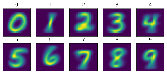
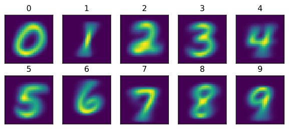
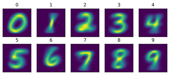
The blur is the naive assumption made visible: the model knows each pixel’s marginal firing rate but nothing about how pixels co-occur, so every sharp stroke smears into an average.
27.7.3.2 Classifying and Evaluating
Prediction sums log-likelihoods per Equation 27.7.6. We precompute \(\log P_{xy}\), \(\log(1-P_{xy})\), and \(\log P_y\), then score a batch of images at once: a pixel that is on contributes \(\log P_{xy}\), a pixel that is off contributes \(\log(1-P_{xy})\), and the prior is added in. The winning class is the \(\mathrm{argmax}\). Before reporting the accuracy, the cell also puts numbers to the underflow story that motivated log space, by checking what the raw products of Equation 27.7.5 would have done in single and double precision.
log_P_xy, log_P_xy_neg = np.log(P_xy), np.log(1 - P_xy)
log_P_y = np.log(P_y)

def scores(X):                       # log p(y) + sum_i log p(x_i|y), per class
    X = X.reshape(-1, 1, 28, 28)                       # (m, 1, 28, 28)
    return (X * log_P_xy + (1 - X) * log_P_xy_neg).reshape(
        len(X), 10, -1).sum(axis=2) + log_P_y

def predict(X):
    return scores(X).argmax(axis=1)

s = scores(X_test)                   # measure what the raw products would do
print(f'float32 underflow: {(np.exp(s.astype(np.float32)) == 0).mean():.1%}'
      f' of class scores; smallest float64 survivor'
      f' = 1e{int(s[np.exp(s) > 0].min() / np.log(10))}')
float((predict(X_test) == Y_test).mean()) # Test accuracyfloat32 underflow: 99.1% of class scores; smallest float64 survivor = 1e-3230.8427float32 underflow: 99.1% of class scores; smallest float64 survivor = 1e-3230.8427float32 underflow: 99.1% of class scores; smallest float64 survivor = 1e-3230.8427float32 underflow: 99.4% of class scores; smallest float64 survivor = 1e-3070.8427Naive Bayes reaches about \(84\%\) accuracy, compared with \(10\%\) for random guessing. Its ten averaged templates cannot represent dependence among pixels, which limits performance on images. Modern neural classifiers model these dependencies and obtain substantially lower error rates.
Images are in fact the hard case for the naive assumption, because adjacent pixels are so tightly coupled. Its canonical home is the opposite regime: bag-of-words text classification, where each feature records whether a given word appears in a document (the Bernoulli event model; the multinomial variant counts occurrences instead) (Manning et al. 2008). There the independence story comes far closer to holding, though it is still not literally true: the presence of any one word out of a vocabulary of tens of thousands says comparatively little about the presence of most others, whereas neighboring pixels almost always agree. The same counting-and-argmax recipe therefore makes naive Bayes a strong, famously cheap baseline for topic labelling and spam filtering, which it dominated for decades (Sahami et al. 1998).
27.7.3.3 Calibration
Three questions remain about the accuracy number, and a generative classifier with a knowingly false assumption is exactly the model to ask them of: how precise is the \(84.27\%\); which mistakes make up the missing \(16\%\); and can the model’s own confidence be trusted? Each takes a few lines.
First, precision. The test accuracy is an estimate computed from \(10{,}000\) random test examples, so it carries a standard error, and the bootstrap of Section 27.5 delivers it exactly as promised there: resample the test indices with replacement, recompute the accuracy on each resample, and read off the spread.
rng = np.random.default_rng(0)
correct = (predict(X_test) == Y_test)                  # per-example 0/1 outcomes
idx = rng.integers(0, len(correct), (1000, len(correct)))  # resampled test sets
boot = correct[idx].mean(axis=1)                       # one accuracy per resample
lo, hi = np.percentile(boot, [2.5, 97.5])
print(f'test accuracy = {correct.mean():.4f}, '
      f'bootstrap 95% CI = ({lo:.4f}, {hi:.4f})')
test accuracy = 0.8427, bootstrap 95% CI = (0.8354, 0.8496)The error bar spans about \(\pm0.7\) accuracy points: the “\(84.27\%\)” is really “\(84.3\%\pm0.7\)”, and the third decimal is noise. One caution about comparisons: this interval quantifies the uncertainty in our model’s accuracy, not the gap to a competitor. Deciding whether another model on the same test set is genuinely better calls for a paired comparison (bootstrap the accuracy difference example by example, or use McNemar’s test); because the two models’ errors are correlated, a competitor whose accuracy falls inside our interval can still be significantly better. Second, the mistakes. A confusion matrix tallies predictions against truth, one row per true digit and one column per predicted digit, and turns the flat error rate into structure.
conf = np.zeros((10, 10), dtype=int)
np.add.at(conf, (Y_test, predict(X_test)), 1)          # tally (true, predicted)
off = conf - np.diag(np.diag(conf))                    # errors only
worst = np.dstack(np.unravel_index(
    np.argsort(off, axis=None)[::-1], (10, 10)))[0][:4]
print('most confused true->predicted:',
      ', '.join(f'{t}->{p} ({off[t, p]})' for t, p in worst))
d2l.plt.imshow(conf, cmap='Blues')
d2l.plt.xlabel('predicted digit')
d2l.plt.ylabel('true digit')
d2l.plt.colorbar();most confused true->predicted: 4->9 (138), 5->3 (106), 8->3 (68), 7->9 (67)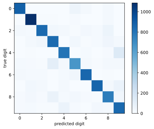
most confused true->predicted: 4->9 (138), 5->3 (106), 8->3 (68), 7->9 (67)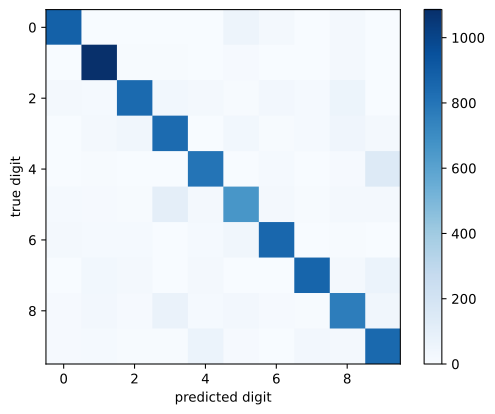
most confused true->predicted: 4->9 (138), 5->3 (106), 8->3 (68), 7->9 (67)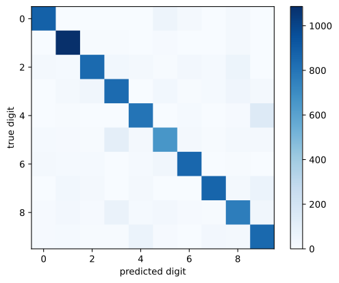
most confused true->predicted: 4->9 (138), 5->3 (106), 8->3 (68), 7->9 (67)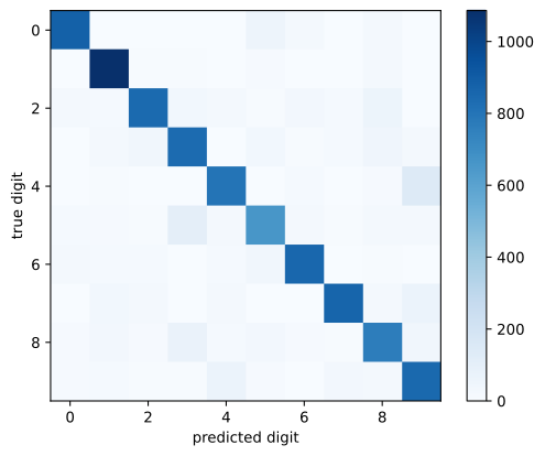
The errors are anything but uniform: the model’s worst failures are \(4\to9\), \(5\to3\), \(8\to3\), and \(7\to9\) (the reverse confusion \(9\to4\) sits just below the printed four). These are largely the digit pairs whose learned templates, plotted above, overlap the most: the most-overlapping pair is indeed the top confusion \(4/9\), though the correspondence is loose rather than exact, as Exercise 6 lets you check. A \(4\) and a \(9\) differ mainly in whether the top strokes close into a loop, a fact carried by the joint behavior of a handful of neighboring pixels; a model that sees only per-pixel marginals is structurally blind to it. The confusion matrix is the independence assumption’s failure map.
Third, the confidence. The class scores determine a genuine posterior: since each score \(s_y(\mathbf x)\) is the logarithm of the Bayes-rule numerator \(p(\mathbf x\mid y)\,p(y)\), exponentiating and normalizing restores the dropped denominator, so \(p(y\mid\mathbf x) = \exp(s_y(\mathbf x))/\sum_{y'}\exp(s_{y'}(\mathbf x))\), a softmax of the scores (Exercise 4 works this out). The model therefore announces a probability along with each predicted digit. A model is calibrated if its announced probabilities match empirical frequencies: among predictions made with confidence \(c\), a fraction \(c\) should be correct. We predicted early in this section that multiplying \(784\) falsely-independent factors would leave the model badly miscalibrated; the cell below checks, binning the test examples by their maximum posterior and comparing the claimed confidence with the achieved accuracy in each bin, the tabular form of a reliability diagram, the standard name for this diagnostic. (The softmax is evaluated in its subtract-the-max stable form from Section 26.5.2.)
s = scores(X_test)
post = np.exp(s - s.max(axis=1, keepdims=True))        # softmax, stably
post /= post.sum(axis=1, keepdims=True)
conf_max = post.max(axis=1)                            # claimed confidence
print(f'mean claimed confidence = {conf_max.mean():.3f},   '
      f'actual accuracy = {correct.mean():.3f}')
for a, b in zip([0.0, 0.9, 0.99, 0.999], [0.9, 0.99, 0.999, 1.0]):
    m = (conf_max > a) & (conf_max <= b)
    print(f'confidence in ({a}, {b}]: {m.sum():5d} examples,  '
          f'claimed {conf_max[m].mean():.4f},  achieved {correct[m].mean():.4f}')
mean claimed confidence = 0.986, actual accuracy = 0.843
confidence in (0.0, 0.9]: 447 examples, claimed 0.7229, achieved 0.3736
confidence in (0.9, 0.99]: 455 examples, claimed 0.9606, achieved 0.4747
confidence in (0.99, 0.999]: 406 examples, claimed 0.9960, achieved 0.5640
confidence in (0.999, 1.0]: 8692 examples, claimed 1.0000, achieved 0.8991On average the model claims \(98.6\%\) confidence while delivering \(84.3\%\) accuracy, and the miscalibration is worst where the claims are strongest: \(87\%\) of all test examples land in the top bin, where the model asserts essentially \(100\%\) certainty yet is right only \(89.9\%\) of the time, and every other bin overstates itself too, with examples announced at \(72\%\) confidence being correct barely \(37\%\) of the time. (The ordering still carries signal, since accuracy does rise with confidence bin, but the probabilities themselves are grossly inflated.) This is exactly what the log-space picture predicts. Each of the \(784\) pixels contributes its log-likelihood ratio to the score as if it were independent evidence, so correlated pixels get counted many times over and the score gaps between classes grow far beyond what the evidence supports: the median gap between the best and second-best class score on the test set is about \(30\) nats (natural-log units; Section 28.2 makes the unit precise), and since \(e^{-30}\approx 10^{-13}\) that already pushes the softmax to \(0\) or \(1\); gaps of hundreds of nats occur only between the best and worst classes. The same failure extends well past naive Bayes: modern neural classifiers trained to low loss are overconfident in the same direction, though to a smaller degree (Guo et al. 2017), which is why the reliability check you just ran, confidence binned against accuracy, is a standard diagnostic for any classifier whose probabilities you intend to consume.
27.7.4 Summary
- Bayes’ rule recasts classification generatively: \(p(y\mid\mathbf{x}) \propto p(\mathbf{x}\mid y)\,p(y)\), predicting the label that maximizes the numerator.
- As a generative model it estimates \(p(\mathbf{x}\mid y)\,p(y)\), the mirror image of a discriminative model like softmax regression, which estimates \(p(y\mid\mathbf{x})\) directly. Sample-efficiency and asymptotic-error comparisons depend on the model families and which assumptions match the data.
- For binary features, the conditional-independence factorization \(p(\mathbf{x}\mid y)=\prod_i p(x_i\mid y)\) replaces \(2^d-1\) class-conditional parameters per class by \(d\). Classification can remain useful even when the resulting probabilities are inaccurate.
- Working in log space avoids the underflow of multiplying hundreds of probabilities. Bernoulli and multinomial naive Bayes have scores affine in their chosen features and therefore linear decision boundaries; Gaussian naive Bayes with class-dependent variances generally has quadratic boundaries.
- Training is maximum likelihood by counting: class priors and per-feature frequencies. Laplace smoothing, \((n_{iy}+1)/(n_y+2)\) for a binary feature, is the posterior mean under a uniform prior (Section 27.3.4.2) and keeps every log-probability finite.
- On MNIST it learns ten averaged digit templates. Conditional dependence and binarization limit this model; sparse bag-of-words text is a common domain in which naive Bayes remains a useful baseline.
- The \(84.27\%\) carries a bootstrap error bar of about \(\pm 0.7\) points; the confusion matrix localizes the failures in template-overlapping pairs like \(4/9\) and \(5/3\); and the model is severely miscalibrated, claiming \(98.6\%\) mean confidence while delivering \(84.3\%\) accuracy, because falsely independent factors double-count correlated evidence. Bin confidence against accuracy (a reliability diagram) before trusting any classifier’s probabilities.
27.7.5 Exercises
- Consider the dataset \(\{(0,0),(0,1),(1,0),(1,1)\}\) with labels given by the XOR of the two coordinates, \(\{0,1,1,0\}\). Compute the naive Bayes estimates \(p(y)\) and \(p(x_i\mid y)\). Does the classifier separate the points? If not, which assumption is violated?
- Suppose we omitted Laplace smoothing and, at test time, an example contained a feature value never observed for some class in training. What would the model’s log-score for that class be, and why?
- The naive Bayes classifier is a special case of a Bayesian network, in which dependencies among random variables are encoded by a graph (see Koller and Friedman (2009)). Explain why adding an explicit edge between the two inputs of the XOR model would let it classify the points correctly.
- The discussion after Equation 27.7.6 showed that each class score of the binary model is affine, \(s_y(\mathbf{x}) = \mathbf{w}_y\cdot\mathbf{x} + b_y\). Derive the exact posterior by normalizing: show that \(p(y\mid\mathbf{x}) = \exp(s_y(\mathbf{x}))\,/\sum_{y'} \exp(s_{y'}(\mathbf{x}))\), and recognize the softmax. Conclude that naive Bayes produces posteriors of exactly the functional form that softmax regression (Section 3.1) fits directly; the two classifiers differ only in how the weights \(\mathbf{w}_y, b_y\) are set. (With two classes, you recover logistic regression.)
- Generalize the smoothing in the training cell to a pseudocount \(\alpha\), estimating \(p(x_i{=}1\mid y)\) as \((n_{iy}+\alpha)/(n_y+2\alpha)\), and report the MNIST test accuracy for \(\alpha\in\{0,1,10\}\). Explain what you observe at \(\alpha=0\): beyond the \(-\infty\) log-probabilities of exercise 2, what does the scoring code compute when a pixel with \(\hat p(x_i{=}1\mid y)=0\) is off in a test image? (Recall that \(0\cdot(-\infty)\) is NaN in floating point.)
- Check the template-overlap explanation of the confusion matrix: flatten the ten smoothed templates in \(P_{xy}\) into vectors and compute the cosine similarity of every pair (one line with NumPy). Which pairs overlap most, and how well do they match the top confusions? You should find that \((4,9)\) is the most similar pair, at cosine similarity about \(0.92\), matching the top confusion, but that the second most similar pair, \((5,8)\) at about \(0.91\), is not among the top four confusions: the correspondence between template overlap and confusion is real but loose.