from d2l import torch as d2l
import torch
from torch import nn6.6 Convolutional Neural Networks (LeNet)
We can now combine convolution, pooling, and fully connected layers into a complete image classifier. In our earlier experiments with image data, we applied a linear model with softmax regression (Section 3.4) and an MLP (Section 4.2) to pictures of clothing in the Fashion-MNIST dataset. To make such data amenable we first flattened each image from a \(28\times28\) matrix into a fixed-length \(784\)-dimensional vector, and thereafter processed them in fully connected layers. Convolutional layers preserve this spatial organization and share parameters across locations, reducing the number of parameters.
This section introduces LeNet, one of the early CNNs to demonstrate strong performance on a practical computer vision task. The model was introduced by (and named for) Yann LeCun, then a researcher at AT&T Bell Labs, for the purpose of recognizing handwritten digits in images (LeCun et al. 1998). This work represented the culmination of a decade of research developing the technology; LeCun’s team published the first study to successfully train CNNs via backpropagation (LeCun et al. 1989).
LeNet matched the performance of support vector machines, then a dominant approach to handwritten-digit recognition, with an error rate below 1% per digit. Variants were deployed to read handwritten amounts on bank checks and deposit slips. The deployment demonstrated that a trained convolutional model could replace a substantial hand-engineered recognition pipeline.
import tensorflow as tf
from d2l import tensorflow as d2l
from d2l import jax as d2l
from flax import nnx
from jax import numpy as jnpfrom d2l import mxnet as d2l
from mxnet import autograd, gluon, init, np, npx
from mxnet.gluon import nn
npx.set_np()6.6.1 LeNet
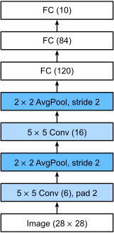
At a high level, LeNet (LeNet-5) consists of two parts: (i) a convolutional encoder consisting of two convolutional layers; and (ii) a dense block consisting of three fully connected layers. The architecture is summarized in Figure 6.6.1.
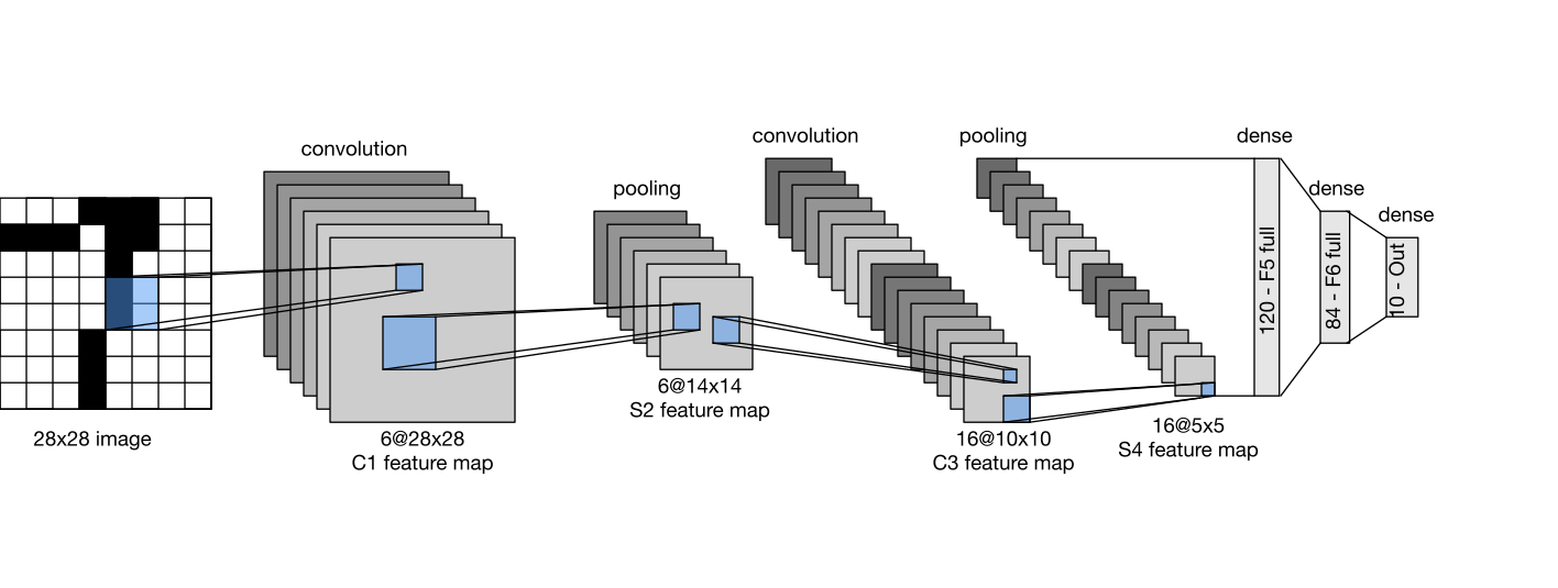
The basic units in each convolutional block are a convolutional layer, a sigmoid activation function, and a subsequent average pooling operation. ReLUs and max-pooling were not part of LeNet-5 and had not yet become the standard choices for trained CNNs. Each convolutional layer uses a \(5\times 5\) kernel and a sigmoid activation function. These layers map spatially arranged inputs to a number of two-dimensional feature maps, typically increasing the number of channels. The first convolutional layer has 6 output channels, while the second has 16. Each \(2\times2\) pooling operation (stride 2) reduces dimensionality by a factor of \(4\) via spatial downsampling. The convolutional block emits an output with shape (batch size, number of channels, height, width) in the PyTorch/MXNet convention; TensorFlow and JAX use the channels-last layout (batch, height, width, channels).
To pass the convolutional block’s output to the dense block, we flatten each example. This transforms the four-dimensional tensor into a matrix whose first axis indexes examples and whose second axis contains the flattened features. LeNet’s dense block has three fully connected layers, with 120, 84, and 10 outputs, respectively. Because we are still performing classification, the 10-dimensional output layer corresponds to the number of possible output classes.
Modern frameworks express LeNet as a Sequential block containing the layers described above. We use Xavier initialization, introduced in Section 4.4.2.2.
def init_cnn(module):
    """Initialize weights for CNNs."""
    if type(module) == nn.Linear or type(module) == nn.Conv2d:
nn.init.xavier_uniform_(module.weight)class LeNet(d2l.Classifier):
"""The LeNet-5 model."""
def __init__(self, lr=0.1, num_classes=10):
super().__init__()
self.save_hyperparameters()
self.net = nn.Sequential(
nn.LazyConv2d(6, kernel_size=5, padding=2), nn.Sigmoid(),
nn.AvgPool2d(kernel_size=2, stride=2),
nn.LazyConv2d(16, kernel_size=5), nn.Sigmoid(),
nn.AvgPool2d(kernel_size=2, stride=2),
nn.Flatten(),
nn.LazyLinear(120), nn.Sigmoid(),
nn.LazyLinear(84), nn.Sigmoid(),
nn.LazyLinear(num_classes))class LeNet(d2l.Classifier):
"""The LeNet-5 model."""
def __init__(self, lr=0.1, num_classes=10):
super().__init__()
self.save_hyperparameters()
self.net = tf.keras.models.Sequential([
tf.keras.layers.Conv2D(filters=6, kernel_size=5,
activation='sigmoid', padding='same'),
tf.keras.layers.AvgPool2D(pool_size=2, strides=2),
tf.keras.layers.Conv2D(filters=16, kernel_size=5,
activation='sigmoid'),
tf.keras.layers.AvgPool2D(pool_size=2, strides=2),
tf.keras.layers.Flatten(),
tf.keras.layers.Dense(120, activation='sigmoid'),
tf.keras.layers.Dense(84, activation='sigmoid'),
tf.keras.layers.Dense(num_classes)])class LeNet(d2l.Classifier):
"""The LeNet-5 model."""
def __init__(self, lr=0.1, num_classes=10, kernel_init=None, rngs=None):
super().__init__()
self.save_hyperparameters(ignore=['rngs', 'kernel_init'])
rngs = nnx.Rngs(d2l.get_key()) if rngs is None else rngs
kernel_init = (nnx.initializers.xavier_uniform() if kernel_init is None
else kernel_init)
self.net = nnx.Sequential(
nnx.Conv(1, 6, kernel_size=(5, 5), padding='SAME',
kernel_init=kernel_init, rngs=rngs),
nnx.sigmoid,
lambda x: nnx.avg_pool(x, window_shape=(2, 2), strides=(2, 2)),
nnx.Conv(6, 16, kernel_size=(5, 5), padding='VALID',
kernel_init=kernel_init, rngs=rngs),
nnx.sigmoid,
lambda x: nnx.avg_pool(x, window_shape=(2, 2), strides=(2, 2)),
lambda x: x.reshape((x.shape[0], -1)), # flatten
nnx.Linear(400, 120, kernel_init=kernel_init, rngs=rngs),
nnx.sigmoid,
nnx.Linear(120, 84, kernel_init=kernel_init, rngs=rngs),
nnx.sigmoid,
nnx.Linear(84, num_classes, kernel_init=kernel_init, rngs=rngs))class LeNet(d2l.Classifier):
"""The LeNet-5 model."""
def __init__(self, lr=0.1, num_classes=10):
super().__init__()
self.save_hyperparameters()
self.net = nn.Sequential()
self.net.add(
nn.Conv2D(channels=6, kernel_size=5, padding=2,
activation='sigmoid'),
nn.AvgPool2D(pool_size=2, strides=2),
nn.Conv2D(channels=16, kernel_size=5, activation='sigmoid'),
nn.AvgPool2D(pool_size=2, strides=2),
nn.Dense(120, activation='sigmoid'),
nn.Dense(84, activation='sigmoid'),
nn.Dense(num_classes))
self.net.initialize(init.Xavier())This is a teaching variant of LeNet-5 rather than an exact historical reproduction. We use \(28\times28\) inputs with padding instead of the original \(32\times32\) inputs, ordinary average pooling instead of trainable subsampling, full connectivity between convolutional channels instead of LeNet-5’s partial C3 connections, logistic sigmoid instead of scaled hyperbolic tangent, and a linear logit head trained with cross-entropy instead of radial-basis output units. These changes keep the alternating convolution–pooling structure and the 6–16–120–84 channel/hidden dimensions while making every component recognizable in a modern library.
We inspect the network by passing a single-channel (black and white) \(28 \times 28\) image through the network and printing the output shape at each layer, we can inspect the model to ensure that its operations line up with what we expect from Figure 6.6.2.
We inspect the network by passing a single-channel (black and white) \(28 \times 28\) image through the network and printing the output shape at each layer, we can inspect the model to ensure that its operations line up with what we expect from Figure 6.6.2.
We inspect the network by passing a single-channel (black and white) \(28 \times 28\) image through the network and printing the output shape at each layer, we can inspect the model to ensure that its operations line up with what we expect from Figure 6.6.2. Because an NNX model already owns its initialized layers, we can pass an array through the callables stored in Sequential and print each intermediate shape directly.
We inspect the network by passing a single-channel (black and white) \(28 \times 28\) image through the network and printing the output shape at each layer, we can inspect the model to ensure that its operations line up with what we expect from Figure 6.6.2.
@d2l.add_to_class(d2l.Classifier)
def layer_summary(self, X_shape):
    X = d2l.randn(*X_shape)
    for layer in self.net:
        X = layer(X)
        print(layer.__class__.__name__, 'output shape:\t', X.shape)

model = LeNet()
model.layer_summary((1, 1, 28, 28))
Conv2d output shape: torch.Size([1, 6, 28, 28])
Sigmoid output shape: torch.Size([1, 6, 28, 28])
AvgPool2d output shape: torch.Size([1, 6, 14, 14])
Conv2d output shape: torch.Size([1, 16, 10, 10])
Sigmoid output shape: torch.Size([1, 16, 10, 10])
AvgPool2d output shape: torch.Size([1, 16, 5, 5])
Flatten output shape: torch.Size([1, 400])
Linear output shape: torch.Size([1, 120])
Sigmoid output shape: torch.Size([1, 120])
Linear output shape: torch.Size([1, 84])
Sigmoid output shape: torch.Size([1, 84])
Linear output shape: torch.Size([1, 10])@d2l.add_to_class(d2l.Classifier)
def layer_summary(self, X_shape):
X = d2l.normal(X_shape)
for layer in self.net.layers:
X = layer(X)
print(layer.__class__.__name__, 'output shape:\t', X.shape)
model = LeNet()
model.layer_summary((1, 28, 28, 1))Conv2D output shape: (1, 28, 28, 6)
AveragePooling2D output shape: (1, 14, 14, 6)
Conv2D output shape: (1, 10, 10, 16)
AveragePooling2D output shape: (1, 5, 5, 16)
Flatten output shape: (1, 400)
Dense output shape: (1, 120)
Dense output shape: (1, 84)
Dense output shape: (1, 10)@d2l.add_to_class(d2l.Classifier)
def layer_summary(self, X_shape):
X = jnp.zeros(X_shape)
for layer in self.net.layers:
X = layer(X)
print(layer.__class__.__name__, 'output shape:\t', X.shape)
model = LeNet()
model.layer_summary((1, 28, 28, 1))Conv output shape: (1, 28, 28, 6)
PjitFunction output shape: (1, 28, 28, 6)
function output shape: (1, 14, 14, 6)
Conv output shape: (1, 10, 10, 16)
PjitFunction output shape: (1, 10, 10, 16)
function output shape: (1, 5, 5, 16)
function output shape: (1, 400)
Linear output shape: (1, 120)
PjitFunction output shape: (1, 120)
Linear output shape: (1, 84)
PjitFunction output shape: (1, 84)
Linear output shape: (1, 10)@d2l.add_to_class(d2l.Classifier)
def layer_summary(self, X_shape):
X = d2l.randn(*X_shape)
for layer in self.net:
X = layer(X)
print(layer.__class__.__name__, 'output shape:\t', X.shape)
model = LeNet()
model.layer_summary((1, 1, 28, 28))Conv2D output shape: (1, 6, 28, 28)
AvgPool2D output shape: (1, 6, 14, 14)
Conv2D output shape: (1, 16, 10, 10)
AvgPool2D output shape: (1, 16, 5, 5)
Dense output shape: (1, 120)
Dense output shape: (1, 84)
Dense output shape: (1, 10)The height and width of the representation at each layer throughout the convolutional block is reduced (compared with the previous layer). The first convolutional layer uses two pixels of padding to compensate for the reduction in height and width that would otherwise result from using a \(5 \times 5\) kernel. As an aside, the image size of \(28 \times 28\) pixels in the original MNIST OCR dataset is a result of trimming two pixel rows (and columns) from the original scans that measured \(32 \times 32\) pixels. This was done primarily to save space (a 30% reduction) at a time when megabytes mattered.
In contrast, the second convolutional layer forgoes padding, and thus the height and width are both reduced by four pixels. As we go up the stack of layers, the number of channels increases layer-over-layer from 1 in the input to 6 after the first convolutional layer and 16 after the second convolutional layer. However, each pooling layer halves the height and width. Finally, each fully connected layer reduces dimensionality, ultimately emitting an output whose dimension matches the number of classes.
6.6.2 Training
We now train the LeNet variant on Fashion-MNIST.
While CNNs have fewer parameters, they can still be more expensive to compute than similarly deep MLPs because each parameter participates in many more multiplications. Using a GPU can accelerate training. The d2l.Trainer class manages device placement and the training loop. By default, it initializes the model parameters on the available devices. As with MLPs, the loss function is cross-entropy, and we minimize it via minibatch stochastic gradient descent.
trainer = d2l.Trainer(max_epochs=10, num_gpus=1)
data = d2l.FashionMNIST(batch_size=128)
model = LeNet(lr=0.1)
model.apply_init([next(iter(data.get_dataloader(True)))[0]], init_cnn)
trainer.fit(model, data)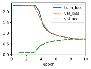
trainer = d2l.Trainer(max_epochs=10)
data = d2l.FashionMNIST(batch_size=128)
with d2l.try_gpu():
    model = LeNet(lr=0.1)
    trainer.fit(model, data)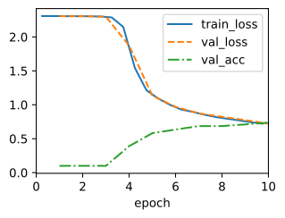
trainer = d2l.Trainer(max_epochs=10, num_gpus=1)
data = d2l.FashionMNIST(batch_size=128)
model = LeNet(lr=0.1)
trainer.fit(model, data)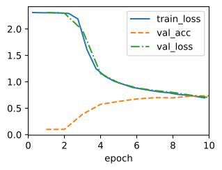
trainer = d2l.Trainer(max_epochs=10, num_gpus=1)
data = d2l.FashionMNIST(batch_size=128)
model = LeNet(lr=0.1)
trainer.fit(model, data)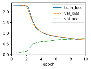
6.6.3 Summary
LeNet combines a convolutional encoder with a small classification head. Its performance on Fashion-MNIST illustrates the advantage of using image structure rather than flattening every input. Modern frameworks also make its implementation substantially shorter than the specialized systems required for the original experiments (Bottou and Le Cun 1988).
The overall encoder–classifier organization remains common, although modern networks replace most of LeNet’s individual components:
| LeNet (1998) | Modern (2020s) | What the change buys |
|---|---|---|
| sigmoid activation | ReLU or GELU | gradients that survive depth instead of saturating |
| average pooling | max-pooling or strided convolution | provides selective or learned local downsampling |
| no normalization | batch or layer normalization | stable activation scales, so much deeper stacks train |
| dense head on flattened features | global average pooling plus one linear layer | removes most of the parameters (the \(400 \times 120\) block here) |
| Xavier initialization | He initialization | variance matched to ReLU rather than to sigmoid |
The next chapter examines these changes through AlexNet (Section 7.1), NiN (Section 7.2.2), batch normalization (Section 7.3), and ResNet (Section 7.4). He initialization, introduced in Section 5.3, accompanies the use of ReLU activations.
6.6.4 Exercises
- [code] Modern components. Retrain
LeNetwith the changes below, using the training settings of this section, and compare the validation accuracy of each variant after 10 epochs with that ofLeNet.- Replace average pooling with max-pooling.
- Replace the sigmoid activations with ReLU.
- Make both changes together, and call the result the modernized LeNet. Which of the two changes accounts for most of the difference in accuracy?
- [code] Architecture sweep. Starting from the modernized LeNet of the first problem, vary one design choice at a time: the convolution window size, the number of output channels of each convolutional layer, and the number of convolutional layers.
- Before training a variant, trace its output shapes with
layer_summaryand count its parameters. Which layer’s parameter count changes most, and why? - Train each variant with the training settings of this section and tabulate its validation accuracy against its parameter count. Does any variant improve on the accuracy of the modernized LeNet?
- Before training a variant, trace its output shapes with
- [code] Original MNIST. Write an
MNISTdata class by adaptingd2l.FashionMNIST, and train bothLeNetand the modernized LeNet of the first problem on it. LeCun et al. (1998) report a test error rate below 1% for LeNet-5 on MNIST.- Compare the test error rates of both networks with this figure.
- For each dataset, compute the difference and the ratio of the two networks’ test error rates, reusing the Fashion-MNIST runs of the first problem. Section 3.2 states that MNIST makes differences among model classes less visible. Does each of the two measures support this statement?
- [code] Activation maps. Train the modernized LeNet of the first problem and extract the feature maps of its first and second convolutional layers, each taken after its ReLU.
- Display them for test images from two different classes, for example pullovers and coats.
- Measure the maximum activation of each of the two layers on Fashion-MNIST test images, on out-of-distribution photos such as a cat or a car, and on uniform random noise. Convert each photo to a \(28 \times 28\) grayscale image, and keep every input in \([0, 1]\), the pixel range of
d2l.FashionMNIST. Do the maxima for photos and noise fall inside or clearly outside the range observed on Fashion-MNIST test images?
- [code] The dense head. ● Table 6.6.1 states that replacing the dense head with global average pooling removes most of LeNet’s parameters.
- Using the weight count of Section 6.4, one bias per output channel or unit, and the layer shapes of Figure 6.6.2, count the parameters of the two convolutional layers combined, of the \(400 \times 120\) dense layer, and of all of
LeNet. What fraction of the total do the convolutional layers account for, and what fraction the \(400 \times 120\) layer? - Replace the entire dense head, from the flatten through the output layer, by global average pooling followed by a single linear layer from 16 to 10 units. How many parameters does the network now have? Before training, predict whether the test accuracy changes by more than one percentage point relative to
LeNet; then retrain and compare. - Instead connect the flattened 400-dimensional convolutional output directly to a ten-way linear output layer. Retrain, and compare the accuracy of the two reduced heads with each other and with your prediction. What does the comparison say about where LeNet’s capacity is used?
- Using the weight count of Section 6.4, one bias per output channel or unit, and the layer shapes of Figure 6.6.2, count the parameters of the two convolutional layers combined, of the \(400 \times 120\) dense layer, and of all of
- [code] Overfitting sanity check. Before trusting a full training run, check that a network can memorize a small dataset. Fix a subset of 50 Fashion-MNIST training images and train on it with all 50 images in one minibatch, for at most 500 gradient steps.
- For both
LeNetand the modernized LeNet of the first problem, record the number of steps until training accuracy exceeds 99%. If a network does not get there, diagnose which architectural or optimization choice is responsible. - Name one bug that this check would catch and one that it would miss, and explain why the check cannot detect the second.
- For both
- Equivariance versus augmentation. A stride-1 convolution on an infinite grid is exactly translation equivariant.
- Go through the layers of
LeNetin order. Name each component that breaks exact translation equivariance of the feature maps, and the components that prevent the final prediction from being translation invariant. - Explain why training
LeNeton translated copies of its training images can improve test accuracy even though its convolutional layers share weights across all locations.
- Go through the layers of