%matplotlib inline
from d2l import torch as d2l
import math
import numpy as np
import random
import torch8.7 Decoding and Generation
The model in Section 8.5 assigns a probability to each possible next token. Producing a sequence requires an additional rule for selecting from these distributions. Always choosing the most probable token often repeats phrases, whereas unconstrained sampling can produce incoherent text.
Decoding comprises the algorithms that turn next-token distributions into sequences (Graves 2013; Holtzman et al. 2020). These algorithms are largely independent of the network and apply to the recurrent models of the next chapter as well as transformer language models.
%matplotlib inline
from d2l import tensorflow as d2l
import math
import numpy as np
import random%matplotlib inline
from d2l import jax as d2l
import math
import numpy as np
import random%matplotlib inline
from d2l import mxnet as d2l
import math
import numpy as np
import random
from mxnet import npx
npx.set_np()8.7.1 The Decoding Problem
A trained language model supplies conditionals: writing \(x_{<t}\) for the prefix \(x_1, \ldots, x_{t-1}\), it turns any prefix into a distribution \(P(x_t \mid x_{<t})\) over the next token. The chain rule of probability assembles these local judgments into the probability of an entire sequence,
\[P(x_1, \ldots, x_T) = \prod_{t=1}^{T} P(x_t \mid x_{<t}). \tag{8.7.1}\]
Decoding asks the inverse question: given the conditionals, which sequence should we output? One natural answer is the most probable sequence, the argmax of Equation 8.7.1 over all candidates. But the number of candidates grows exponentially. With vocabulary \(\mathcal{V}\) and \(T\) tokens to generate there are \(|\mathcal{V}|^T\) sequences to compare; for our modest 1,024-token vocabulary and a 50-token continuation that is \(1024^{50} = 2^{500} \approx 10^{150}\) sequences. Exhaustive search is therefore infeasible. A practical decoder evaluates only a small subset of prefixes and must decide which ones to retain at each step.
Intractability is only half of the problem, though. The other half is that for many uses the most probable sequence is not even what we want. When a task has a narrow set of acceptable answers conditioned on the input, as in transcription, searching for a high-probability sequence is often useful. This is a model-level decision rule, not necessarily the task-optimal rule: translation may have several valid references, and length or utility can matter in addition to model probability. For open-ended writing there are many acceptable continuations, each individually improbable. A model that has learned this diversity spreads its mass accordingly, and insisting on the single most probable output discards the diversity we asked for; we will see shortly that it collapses into dull repetition. Sampling instead matches the output’s diversity to the model’s.
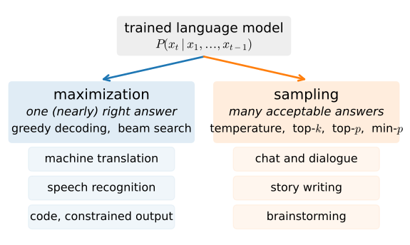
These two families organize the methods in this section (Figure 8.7.1). Maximization methods, including greedy decoding and beam search, seek high-probability outputs and are common when the acceptable output set is narrow. Sampling methods draw from the model’s distribution, reshaped by a small set of dials named temperature, top-\(k\), top-\(p\), and min-\(p\), and dominate open-ended generation: chat, stories, and dialogue. Applications can also combine search, sampling, and task-specific reranking.
8.7.1.1 A Model to Decode From
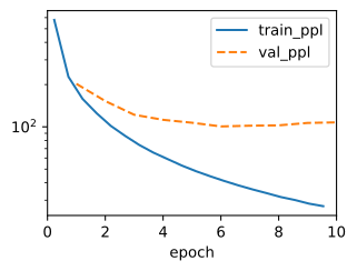
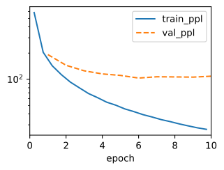
We need a trained model to experiment on, and the concise RNN language model of Section 8.5 is ideal: small enough to train here in about a minute, good enough (recall, about 2.4 bits per byte) that its continuations respond visibly to decoding choices. We retrain it with the same training procedure used there.
data = d2l.TimeMachine(batch_size=1024, num_steps=32,
num_train=50000, num_val=5000)rnn = d2l.RNN(num_inputs=64, num_hiddens=128)
model = d2l.RNNLM(rnn, vocab_size=len(data.vocab), lr=4)with d2l.try_gpu():
rnn = d2l.RNN(num_inputs=64, num_hiddens=128)
model = d2l.RNNLM(rnn, vocab_size=len(data.vocab), lr=4)rnn = d2l.RNN(num_inputs=64, num_hiddens=128)
model = d2l.RNNLM(rnn, vocab_size=len(data.vocab), lr=4)rnn = d2l.RNN(num_inputs=64, num_hiddens=128)
model = d2l.RNNLM(rnn, vocab_size=len(data.vocab), lr=4)trainer = d2l.Trainer(max_epochs=10, gradient_clip_val=1, num_gpus=1)
model.board.yscale = 'log'
trainer.fit(model, data)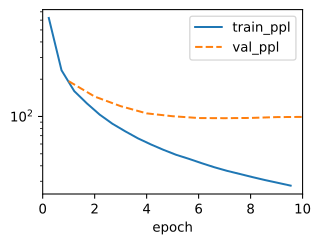
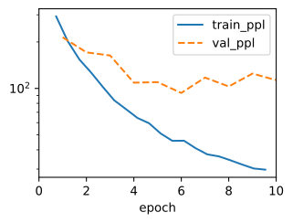
Every decoding strategy in this section interacts with the model through one narrow interface: hand me the token ids so far, and I will hand you the logits for the next token. We wrap the trained network in a step_fn implementing that interface, converting the result to a plain NumPy vector so that the strategies themselves can be written once, in ordinary Python, with no framework in sight. Every algorithm below can decode any model that fills this interface: today’s RNN, next chapter’s LSTM, a transformer.
def step_fn(ids):  # Token ids in, numpy logits for the next token out
    with torch.no_grad():
        logits = model(d2l.tensor([ids], device=d2l.try_gpu()))
    return d2l.numpy(logits)[0, -1]
def step_fn(ids): # Token ids in, numpy logits for the next token out
logits = model(d2l.tensor([ids]))
return d2l.numpy(logits)[0, -1]def step_fn(ids): # Token ids in, numpy logits for the next token out
logits = model(d2l.tensor([ids]))
return d2l.numpy(logits)[0, -1]def step_fn(ids): # Token ids in, numpy logits for the next token out
logits = model(d2l.tensor([ids], ctx=d2l.try_gpu()))
return d2l.numpy(logits)[0, -1]Note the deliberate extravagance: each call re-runs the network over the entire prefix just to produce one vector of logits. We will tally the cost of this convenience at the end of the section.
8.7.2 Greedy Decoding
The simplest decoder commits, at every step, to the single most likely token:
\[x_t = \operatorname*{argmax}_{x \in \mathcal{V}} P(x \mid x_{<t}).\]
The algorithm is a one-line loop: score, take the argmax, append, repeat. It costs one model evaluation per token, \(\mathcal{O}(|\mathcal{V}| T)\) work in total, and it is deterministic: the same prefix always yields the same continuation.
def decode_greedy(text, num_tokens=50):
    ids = data.tokenizer.encode(text)
    for _ in range(num_tokens):
        ids.append(int(step_fn(ids).argmax()))
    return data.tokenizer.decode(ids)

for text in ('the time traveller', 'it seemed to me that'):
d2l.print_wrapped(repr(decode_greedy(text)))"the time traveller to\nthe Time Traveller's\ndeliumerable\nchanism.
The\ndisappo, and\ntherempatural\nflted to\nshalls of\nwerest"
"it seemed to me that the\nsunnome to\ntowards the\nsunnels.\n\n'In
a\nsharping\nof the\nlittle-side, and\ntherentrely"'the time traveller. The\ndismins of my faint\ntheseen. It was not the
circle of the little people. And the Time Traveller hesitated\ntheirer.
I had\navidently a'
'it seemed to me that my fy-fastly in a friendron\nbranent the Time Machine,
and, I found a corner of the floor, and then\nthere in a pattering, and
then'"the time traveller to the gallery of my\nfour ornow a certain was a
starting my\nman,\nincured, I had\nthe signs of the Time
Traveller.\n\n'I wo"
"it seemed to me that the Time Traveller, the bigned. I felt a
trames.\n\n'In that the Time Traveller.\n\n'I wondering in
the\nsheert.\n\n'In that"'the time traveller,\nI could see no\nsideways,\nI could see
no\nsideways,\nI could see no\nsideways,\nI could see no\nsideways,\nI
could see no'
'it seemed to me that\nthese,\nand straighter I had\nchairing,\nI could see
no\nsideways,\nI could see no\nsideways,\nI could see no\nsideways'The output is locally plausible Wells, but it drifts toward the generic, and it drifts predictably: the two different prefixes soon funnel into the same stock phrases, and, depending on the training run, the continuation may lock into a verbatim repeating cycle outright. Two distinct flaws are on display. The first is myopia: a sequence of locally best tokens need not be the best sequence. Suppose the vocabulary holds four tokens \(A\), \(B\), \(C\), and \(D\), and at the first step the model assigns them probabilities 0.5, 0.2, 0.2, and 0.1. Greedy picks \(A\). Conditioned on \(A\), suppose the best continuation runs through \(B\) with probability 0.4, then 0.4, then 0.6: the greedy sequence has probability \(0.5 \times 0.4 \times 0.4 \times 0.6 = 0.048\). Had we accepted the second-best token \(C\) (probability 0.3) at the second step, the changed conditioning might offer 0.6 and 0.6 next, for a total of \(0.5 \times 0.3 \times 0.6 \times 0.6 = 0.054\). Taking one locally suboptimal step bought a globally better sequence; greedy can never make that trade.
The second flaw runs deeper than myopia. Greedy decoding feeds its own argmax back in as context, and repetition is self-reinforcing: once a phrase has appeared twice, its third occurrence is more probable still, since the model has learned that text which repeats tends to keep repeating. The argmax feedback loop rides this gradient toward repetition and, given enough maximization pressure, into a literal fixed cycle. Holtzman et al. (2020) documented the phenomenon, aptly named neural text degeneration, in models a thousand times larger than ours: maximization-based decoding of open-ended text produces output that is repetitive, low-diversity, and measurably unlike human text, no matter how good the underlying model is. Keep that in mind as we now fix the first flaw, myopia, and watch the second one get worse.
8.7.3 Beam Search
Decoding strategies live on a spectrum between the two extremes we have met: greedy search commits instantly and exhaustive search never commits at all. Beam search interpolates with a single knob, the beam size \(k\): keep the \(k\) most probable prefixes alive at every step. At the first step it selects the \(k\) highest-probability tokens; thereafter, each of the \(k\) surviving prefixes is extended by every token in the vocabulary, the resulting \(k \cdot |\mathcal{V}|\) candidates are scored by their cumulative log-probability, and only the best \(k\) survive. Greedy search is the special case \(k = 1\); exhaustive search is the limit where \(k\) outgrows the candidate count and pruning never happens.
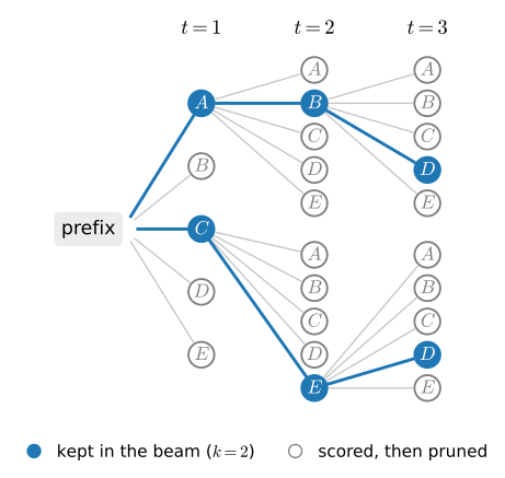
Figure 8.7.2 traces a worked example with \(k = 2\) over the toy vocabulary \(\mathcal{V} = \{A, B, C, D, E\}\) and three generation steps. Suppose the two most probable first tokens are \(A\) and \(C\); they form the initial beam. At the second step we compute, for every \(x_2 \in \mathcal{V}\), the extension scores
\[\begin{aligned}P(A, x_2 \mid x_{\leq m}) &= P(A \mid x_{\leq m}) P(x_2 \mid A, x_{\leq m}),\\ P(C, x_2 \mid x_{\leq m}) &= P(C \mid x_{\leq m}) P(x_2 \mid C, x_{\leq m}),\end{aligned} \tag{8.7.2}\]
ten numbers in all (here \(x_{\leq m}\) denotes the given prefix), and keep the two largest, say \(P(A, B \mid x_{\leq m})\) and \(P(C, E \mid x_{\leq m})\). The third step repeats the calculation from the survivors \(AB\) and \(CE\), yielding say \(ABD\) and \(CED\). Note what pruning bought us: instead of \(5^3 = 125\) sequences we scored \(5 + 10 + 10 = 25\), and in general beam search costs \(\mathcal{O}(k |\mathcal{V}| T)\), a factor \(k\) more than greedy and exponentially less than exhaustive search.
One correction is needed before we can rank the finished candidates. Log-probabilities of tokens are non-positive, so the cumulative score of a sequence only falls as it grows, and comparing raw scores systematically favors short candidates (an acute issue once an end-of-sequence token can terminate some beams early). The standard remedy is length normalization (Wu et al. 2016): rank each candidate of generated length \(L\) by
\[\frac{1}{L^\alpha} \sum_{t=m+1}^{m+L} \log P(x_t \mid x_{<t}), \tag{8.7.3}\]
where \(\alpha\) (typically around 0.75) interpolates between no correction (\(\alpha = 0\)) and the per-token average log-probability (\(\alpha = 1\)). The implementation below follows this procedure directly. Finished candidates (those that produced eos_id) pass through unchanged from round to round; live ones are expanded and rescored. Since the global top \(k\) can contain at most \(k\) continuations of any single prefix, it suffices to consider each beam’s \(k\) best tokens rather than all \(|\mathcal{V}|\) of them. Like the rest of this section’s toolkit, everything is plain Python against plain arrays, so this same function will decode next chapter’s translation model without modification.
def beam_search(step_fn, prefix, num_tokens, beam_size=4,
                alpha=0.75, eos_id=None):
    """Length-normalized beam search (score = log P / len^alpha).
    Returns candidates sorted best-first; [0][1] is the argmax sequence."""
    def log_softmax(logits):
        logits = [float(l) for l in logits]
        m = max(logits)
        lse = m + math.log(sum(math.exp(l - m) for l in logits))
        return [l - lse for l in logits]
    score = lambda logp, ids: logp / max(1, len(ids) - len(prefix))**alpha
    beams = [(0.0, list(prefix), False)]  # (log-prob, sequence, finished)
    for _ in range(num_tokens):
        if all(done for _, _, done in beams):
            break
        candidates = [b for b in beams if b[2]]  # Finished pass through
        for logp, ids, _ in (b for b in beams if not b[2]):
            logprobs = log_softmax(step_fn(ids))
            best = sorted(range(len(logprobs)),
                          key=lambda i: -logprobs[i])[:beam_size]
            candidates += [(logp + logprobs[i], ids + [i], i == eos_id)
                           for i in best]
        beams = sorted(candidates, key=lambda b: score(b[0], b[1]),
                       reverse=True)[:beam_size]
    return sorted([(score(logp, ids), ids) for logp, ids, _ in beams],
                  reverse=True)
Let’s decode the same two prefixes as before, with \(k = 1\) (which reproduces greedy decoding) and \(k = 4\). To make the repetition failure measurable rather than anecdotal we also report distinct-3, the fraction of distinct 3-grams among all 3-grams of the continuation: a value of 1 means no 3-gram ever recurs, and a continuation stuck in a loop scores close to 0.
def distinct(ids, n=3):
    grams = [tuple(ids[i:i + n]) for i in range(len(ids) - n + 1)]
    return len(set(grams)) / max(1, len(grams))

for text in ('the time traveller', 'it seemed to me that'):
    pre = data.tokenizer.encode(text)
    for k in (1, 4):
        score, ids = beam_search(step_fn, pre, 40, beam_size=k)[0]
        d2l.print_wrapped(f'k={k}, score {score:.2f}, distinct-3 '
                          f'{distinct(ids[len(pre):]):.2f}: '
f'{data.tokenizer.decode(ids)!r}')k=1, score -4.75, distinct-3 1.00: "the time traveller to\nthe Time
Traveller's\ndeliumerable\nchanism. The\ndisappo,
and\ntherempatural\nflted to"
k=4, score -3.49, distinct-3 0.34: "the time traveller.\n\n'As
the\nsunnels.\n\n'As the\nsunnels.\n\n'As the\nsunnels."
k=1, score -4.44, distinct-3 0.92: "it seemed to me that the\nsunnome
to\ntowards the\nsunnels.\n\n'In a\nsharping\nof the\nlittle-"
k=4, score -3.54, distinct-3 0.61: "it seemed to me that ifuppose.\n\n'As
the\nsunnels.\n\n'As the\nsunnels.\n\n'Then I had seen"k=1, score -4.59, distinct-3 1.00: 'the time traveller. The\ndismins of my
faint\ntheseen. It was not the circle of the little people. And the Time
Traveller hesitated\ntheir'
k=4, score -3.52, distinct-3 0.82: "the time traveller.
The\ndisappeared.\n\n'There I found a gallery,\nchanismory.\n\n'There I
found a secondit"
k=1, score -5.08, distinct-3 1.00: 'it seemed to me that my fy-fastly in a
friendron\nbranent the Time Machine, and, I found a corner of the floor,
and then\nthe'
k=4, score -3.59, distinct-3 0.95: "it seemed to me that the flooral\npoint.
The\ndisappeared.\n\n'There I found a gallery,\nchanismory.\n\n'"k=1, score -4.76, distinct-3 1.00: 'the time traveller to the gallery of
my\nfour ornow a certain was a starting my\nman,\nincured, I had\nthe
signs of'
k=4, score -3.90, distinct-3 0.87: "the time traveller tow, I saw that I
had\nlooked at first.\n\n'There I found a second.\n\n'There I don't know
how it was"
k=1, score -4.39, distinct-3 0.89: "it seemed to me that the Time Traveller,
the bigned. I felt a trames.\n\n'In that the Time Traveller.\n\n'I
wondering in the\ns"
k=4, score -3.81, distinct-3 0.76: "it seemed to me that the Time
Traveller.\n\n'Well, I saw it.\n\n'As I stood there in the
end.\n\n'Well, I saw that I was in\nthe"k=1, score -4.95, distinct-3 0.29: 'the time traveller,\nI could see
no\nsideways,\nI could see no\nsideways,\nI could see no\nsideways,\nI
could see no\n'
k=4, score -4.14, distinct-3 0.63: 'the time travellerlearly
enough\ndisappeared to me, as I say, I\nfirst I\ndisappeared to me, as I
say, I\nfurther me'
k=1, score -4.80, distinct-3 0.74: 'it seemed to me that\nthese,\nand
straighter I had\nchairing,\nI could see no\nsideways,\nI could see
no\nsideways,'
k=4, score -4.29, distinct-3 0.82: 'it seemed to me that they
were\nsomething\nhimbstance, I\nfirst I\ndisappeared to me, as I say,
I\nfirst I\ndism'Beam search mostly does what it promises: at \(k = 4\) it usually finds continuations that the model scores better than the greedy ones, curing the myopia of the four-token example above. It remains an approximate search, though, so on a given prefix a wider beam can occasionally come back worse. And yet look at the text. The continuations it returns fall back on the same phrase again and again, sometimes into a literal loop, and the wider beam’s distinct-3 numbers drop below the greedy ones and far below the values sampling will achieve, sharply so in some frameworks: the extra search buys a higher-probability loop to be stuck in. This is the degeneration mechanism at work: the better a maximizer gets, the deeper it digs into the repetitive mode of the distribution. The lesson generalizes far beyond RNNs. For open-ended text the argmax itself is a bad target, and no improvement in search can fix a correctly solved wrong problem (Holtzman et al. 2020).
It is tempting to conclude that more search at least helps the tasks where maximization is the right target. Curiously, it does not: in machine translation, pushing the beam from a handful to hundreds reliably lowers translation quality. Ever-larger beams find ever-higher-probability outputs, and those outputs are systematically shorter and blander, until the search starts uncovering pathologies of the model itself, such as an empty translation that outscores every real one. Length normalization softens this large-beam curse without eliminating it, so practitioners stop at small beams, typically \(k\) between 4 and 10, where the search fixes local myopia but is not yet strong enough to exploit the model’s blind spots.
Where does beam search live today? Exactly where its assumptions hold: speech recognition and machine translation systems (Sutskever et al. 2014; Wu et al. 2016) still beam-decode, and lexically constrained decoding, which forces given words or phrases into the output, runs beam search over the continuations that make progress on those constraints. Constraints on the output’s form, such as a grammar, a JSON schema, or an API signature, are usually enforced instead by masking, at every step, the tokens that would make the output invalid, which works with any decoder. Your chat assistant, however, does not use beam search: open-ended dialogue sits firmly in the second family, to which we now turn.
8.7.4 Sampling and Its Dials
If the model’s distribution is worth trusting, the principled way to generate is to sample from it: draw \(x_t \sim P(x_t \mid x_{<t})\), append, repeat. Text produced this way is distributed exactly as the model believes text should be, with all the diversity that maximization threw away and none of its repetition patterns. The remaining problem lies in the tail. Our model spreads small probability over a thousand tokens, a large model over hundreds of thousands, and although each unlikely token is individually negligible, their combined mass at every step is not. Sampling therefore regularly hits tokens the model itself considers near-nonsense, and one absurd token, fed back as context, can derail everything after it. Holtzman et al. (2020) call this the unreliable tail: the model’s estimates are relatively trustworthy at the head of the distribution and mostly noise far down the ranking, so the fix is to sample from a reshaped, truncated distribution. Each of the dials below is one way of doing that.
Temperature rescales before sampling. Dividing every logit \(o_x\) by a temperature \(T > 0\) gives
\[P_T(x \mid x_{<t}) = \frac{\exp(o_x / T)}{\sum_{x' \in \mathcal{V}} \exp(o_{x'} / T)} \propto P(x \mid x_{<t})^{1/T}. \tag{8.7.4}\]
At \(T = 1\) we sample the model as-is; as \(T \to 0\) the distribution sharpens toward its mode and sampling becomes greedy decoding; as \(T\) grows it flattens toward uniform. Temperature trades diversity against safety smoothly, but it reshapes head and tail together: cooling the distribution enough to suppress the tail also crushes legitimate variety at the head.
Top-\(k\) truncates by count: keep the \(k\) most probable tokens, renormalize, and sample (Radford et al. 2019). Top-\(p\) (or nucleus) sampling truncates by mass: keep the smallest set of most-probable tokens whose cumulative probability reaches \(p\), for example \(p = 0.9\) (Holtzman et al. 2020). The difference matters because the model’s confidence varies wildly from step to step. Where our model is nearly certain of the next token, a fixed \(k = 20\) needlessly admits nineteen bad options; mid-sentence, where dozens of words are genuinely plausible, the same \(k\) may cut off real diversity. Top-\(p\) adapts better, keeping few tokens when the head is heavy and many when it is flat, but it too misbehaves on peaked distributions: if the top token already holds 0.95 of the mass, top-\(p\) with \(p = 0.9\) keeps exactly one token and acts greedily even where the runner-up was perfectly acceptable.
Min-\(p\) scales the cutoff by the model’s own confidence (Nguyen et al. 2025): keep every token whose probability is at least \(p_{\min}\) times that of the most probable token, e.g. \(p_{\min} = 0.05\). When the model is sure, the bar is high and few tokens pass; when the model is uncertain, the bar drops and the genuine variety survives. This relative rule holds up notably better at high temperatures, where creative sampling wants to operate and where absolute-threshold rules admit the noise floor wholesale.
8.7.4.1 A Unified Sampler
All four dials act on the same object, the next-token distribution, so a single function can host them. sample_next turns one vector of logits into one token id: greedy if asked, otherwise temperature-scaled sampling after optional top-\(k\), top-\(p\), and min-\(p\) truncation. Note how each truncation rule is just a different cut of the same sorted-by-probability order, a pure function of the distribution; we exploit that shortly to visualize all three at once. Like beam_search it is written in plain Python, and it draws through an explicit rng (anything with a random() method, such as numpy.random.default_rng(seed)) so that generation is reproducible.
def sample_next(logits, strategy='greedy', temperature=1.0,
                k=None, p=None, min_p=None, rng=None):
    """Choose the next token id from a 1-D numpy logits array.
    strategy: 'greedy' | 'sample' (with optional top-k / top-p / min-p
    truncation applied to the temperature-scaled distribution)."""
    logits = [float(l) for l in logits]
    if strategy == 'greedy' or temperature == 0:
        return max(range(len(logits)), key=lambda i: logits[i])
    m = max(logits)
    probs = [math.exp((l - m) / temperature) for l in logits]
    total = sum(probs)
    probs = [q / total for q in probs]
    order = sorted(range(len(probs)), key=lambda i: -probs[i])
    keep = len(order)
    if k is not None:  # Top-k: the k most probable tokens
        keep = min(keep, k)
    if p is not None:  # Top-p: smallest head with cumulative mass >= p
        mass, n = 0.0, 0
        while mass < p and n < len(order):
            mass, n = mass + probs[order[n]], n + 1
        keep = min(keep, n)
    if min_p is not None:  # Min-p: within a factor of the top token
        bar = min_p * probs[order[0]]
        keep = min(keep, sum(q >= bar for q in probs))
    kept = order[:keep]
    rng = random if rng is None else rng
    r = rng.random() * sum(probs[i] for i in kept)
    for i in kept:
        r -= probs[i]
        if r <= 0:
            return i
    return kept[-1]
generate is the loop we have been writing by hand all along: query step_fn, choose via sample_next (extra keyword arguments pass straight through to it), append, and stop early if an end-of-sequence token appears. Open-ended generation has no such token, so our demonstrations simply run for a fixed length; the translation models of the next chapter set eos_id and let the model decide when it is done.
def generate(step_fn, prefix, num_tokens, eos_id=None, **strategy):
    """Autoregressive generation. step_fn(ids: list[int]) -> numpy logits
    for the next token. Returns prefix + continuation (stops on eos_id)."""
    ids = list(prefix)
    for _ in range(num_tokens):
        ids.append(sample_next(step_fn(ids), **strategy))
        if eos_id is not None and ids[-1] == eos_id:
            break
    return ids
A toy distribution makes the truncation rules concrete. Five tokens carry probabilities 0.45, 0.25, 0.15, 0.10, and 0.05. Top-\(k\) with \(k = 2\) may only ever emit tokens 0 and 1; top-\(p\) with \(p = 0.85\) keeps three tokens, since the cumulative mass first reaches 0.85 at the third; min-\(p\) with \(p_{\min} = 0.5\) keeps the tokens with probability at least \(0.5 \times 0.45 = 0.225\), which is again tokens 0 and 1.
logits, rng = np.log([0.45, 0.25, 0.15, 0.1, 0.05]), np.random.default_rng(0)
print('greedy:', sample_next(logits))
for dial in (dict(k=2), dict(p=0.85), dict(min_p=0.5)):
    draws = [sample_next(logits, strategy='sample', rng=rng, **dial)
             for _ in range(15)]
    print(dial, draws)
greedy: 0
{'k': 2} [0, 0, 0, 0, 1, 1, 0, 1, 0, 1, 1, 0, 1, 0, 1]
{'p': 0.85} [0, 2, 1, 0, 0, 0, 0, 1, 1, 1, 0, 2, 2, 1, 1]
{'min_p': 0.5} [1, 0, 0, 1, 0, 0, 0, 1, 1, 0, 0, 0, 0, 0, 0]8.7.4.2 One Distribution, Three Cutoffs
We now examine the distribution modified by each decoding parameter. We query the trained model once and plot its entire next-token distribution, sorted by decreasing probability, on logarithmic axes (the shape is Zipf-like, as Section 8.3 would lead us to expect). On this plot each truncation rule is a single line. Top-\(k\) is a vertical cut at rank \(k\), wherever the probabilities happen to lie. Top-\(p\) is a vertical cut at the rank where the cumulative mass reaches \(p\), so its position slides with the shape of the head. Min-\(p\) is a horizontal cut at \(p_{\min}\) times the top probability: every token above the line survives, and the line itself rides up and down with the model’s confidence. Everything below and to the right of the cuts is the unreliable tail that truncation exists to remove.
def next_probs(text):  # Sorted next-token distribution after a prefix
    logits = step_fn(data.tokenizer.encode(text))
    probs = np.exp(logits - logits.max())
    return np.sort(probs / probs.sum())[::-1]

probs = next_probs('the time traveller')
n_p = int((np.cumsum(probs) < 0.9).sum()) + 1
n_m = int((probs >= 0.05 * probs[0]).sum())
d2l.set_figsize((5.5, 3))
d2l.plt.loglog(np.arange(1, len(probs) + 1), probs, color='C0')
d2l.plt.axvline(20, color='C1', ls='--', label='top-k, k=20')
d2l.plt.axvline(n_p, color='C2', ls='-.', label=f'top-p=0.9: keep {n_p}')
d2l.plt.axhline(0.05 * probs[0], color='C3', ls=':',
                label=f'min-p=0.05: keep {n_m}')
d2l.plt.xlabel('token rank')
d2l.plt.ylabel('probability')
d2l.plt.legend()<matplotlib.legend.Legend at 0x75df62fc6c60>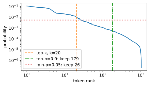
<matplotlib.legend.Legend at 0x7e301814afc0>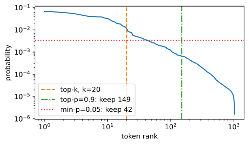
<matplotlib.legend.Legend at 0x738fd0398410>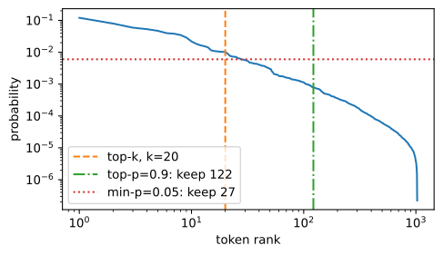
<matplotlib.legend.Legend at 0x7430f112b830>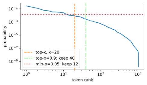
The adaptivity argument is now checkable: apply the same dials after two different prefixes and compare the kept sets. Top-\(k\) keeps twenty tokens regardless. The other two rules track the model’s confidence: the more certain the model, the smaller the top-\(p\) and min-\(p\) sets tend to be. (How confident the model is after a given prefix varies from training run to training run; the printed top probability tells you what this one thinks.) That is the behavior we wanted: strict where the model is sure, permissive where it is genuinely uncertain.
for text in ('the time traveller', 'it seemed to me that'):
    probs = next_probs(text)
    n_p = int((np.cumsum(probs) < 0.9).sum()) + 1
    n_m = int((probs >= 0.05 * probs[0]).sum())
    print(f'{text!r}: top prob {probs[0]:.2f}, top-k keeps 20, '
f'top-p keeps {n_p}, min-p keeps {n_m}')'the time traveller': top prob 0.14, top-k keeps 20, top-p keeps 103, min-p keeps 23
'it seemed to me that': top prob 0.10, top-k keeps 20, top-p keeps 160, min-p keeps 39'the time traveller': top prob 0.25, top-k keeps 20, top-p keeps 141, min-p keeps 6
'it seemed to me that': top prob 0.07, top-k keeps 20, top-p keeps 155, min-p keeps 52'the time traveller': top prob 0.15, top-k keeps 20, top-p keeps 80, min-p keeps 16
'it seemed to me that': top prob 0.17, top-k keeps 20, top-p keeps 142, min-p keeps 19'the time traveller': top prob 0.22, top-k keeps 20, top-p keeps 105, min-p keeps 13
'it seemed to me that': top prob 0.12, top-k keeps 20, top-p keeps 224, min-p keeps 308.7.4.3 The Same Prefix Under Every Strategy
Time to hear the dials rather than plot them. First, temperature alone: at \(T = 0.5\) the text hugs the model’s mode and inherits some of greedy’s repetitiveness, at \(T = 1\) it is diverse but occasionally derails into tail nonsense, and as the temperature rises the sampler starts reaching for tokens whose bytes no longer decode to valid text (the replacement characters below), until at \(T = 2\) the flattened distribution produces gibberish outright.
prefix = data.tokenizer.encode('the time traveller')
for T in (0.5, 1.0, 2.0):
    out = generate(step_fn, prefix, 50, strategy='sample', temperature=T,
                   rng=np.random.default_rng(0))
d2l.print_wrapped(f'T={T}: {data.tokenizer.decode(out)!r}')T=0.5: 'the time traveller the\nsunning to believe and frog,\nof a\nlittle-
fournalk and fast\nwerently to me, there is\ntherempoint of the P'
T=1.0: 'the time traveller\nbutterus had e are l; and everything all\nout
was\nwerest I just that\x1b me from be discondualar of pra though to
fairothes moraryed about'
T=2.0: "the time travellerive formerachin\x14 whitetingreost mini Then, its
knowade back with like\ning chan nworldmsychologistasable my
wasurdfterishibqu C�,' spur ruway r'ic before wasark"T=0.5: 'the time travellermmentered the little people of the
great\npreciedred theseeds. But, no right. Twy\npresently a bothes.
There were no turning of right. I did'
T=1.0: "the time travellerying to freour little proper maty. Fearising car
in a half-conaring,'ac they outerrid you rather- in him to clotarerired,
then, man"
T=2.0: 'the time traveller aduded byureshingationsoratoryrto there ofove gr
way\n so uponul by the Time perx by haak� but crefter fter wag she
theyX� be these bish by histherin moon Inot'T=0.5: 'the time travellerfushes, too, and in the first time, I found that I
thought in a moment, was a smallerne; to the little people. I thought of
the mereasonable, I was express the breat'
T=1.0: 'the time travellereli, and po sl more kelys. Yet again, moret in
this strange. Yet all ofently still sur. Stor. There were\nBexason. It
was\nfor a creatureion'
T=2.0: 'the time travelleroneyed inff*gg riedH Man I uses night isile
suingocent before hill could sGched smoneting you all dim unifbe gl� lur
after d gourH at everyrilog'T=0.5: 'the time traveller,\nI could nothing\nhandant dimensiting
at\nwarception,\nand,\nby sleeping,\ntherever\nwhat Time Traveller,\nand
everinger\nwere,'
T=1.0: 'the time traveller had been\nthe skyound, lawnve
their\nhadmadeacadeast\nban, unaknesser�ide bingmentsideageedell you
follow now,, so touchedtimes them\nwor'
T=2.0: 'the time traveller reance tendich distical shaally( futi enough,
felt c white frow from\nlearhin after these\\oseonoveking waste do lau
atationhingWow Weena wouldfat downering of gom minute'Finally, the whole menu on one prefix, with the distinct-3 diversity score alongside. Greedy is deterministic and generic, when not stuck in a loop outright; pure sampling is diverse but erratic; the truncated samplers occupy the useful middle, keeping the diversity that maximization destroyed (their distinct-3 stays near 1) while cutting the tail that pure sampling trips over. This is why some combination of temperature with top-\(p\) or min-\(p\) is the default in essentially every deployed text generator today.
strategies = {'greedy': dict(strategy='greedy'),
              'T=1.0': dict(strategy='sample'),
              'top-k': dict(strategy='sample', k=20),
              'top-p': dict(strategy='sample', p=0.9),
              'min-p': dict(strategy='sample', min_p=0.05)}
for name, s in strategies.items():
    out = generate(step_fn, prefix, 50, rng=np.random.default_rng(0), **s)
    d2l.print_wrapped(f'{name:>7} (distinct-3 '
                      f'{distinct(out[len(prefix):]):.2f}): '
f'{data.tokenizer.decode(out)!r}') greedy (distinct-3 1.00): "the time traveller to\nthe Time
Traveller's\ndeliumerable\nchanism. The\ndisappo,
and\ntherempatural\nflted to\nshalls of\nwerest"
T=1.0 (distinct-3 1.00): 'the time traveller\nbutterus had e are l; and
everything all\nout was\nwerest I just that\x1b me from be discondualar
of pra though to fairothes moraryed about'
top-k (distinct-3 1.00): 'the time traveller,\nthey deacesoned\ngouseingly
an\nvention of\ntheeral.\nnel; for me\nsheredalist was solerimbs. One
corce'
top-p (distinct-3 1.00): 'the time traveller in\ndisx him more Busure,
there is " Is of metaly--back alme!thditions. The Editor in which lit
from\ntheimare people me.\nThe'
min-p (distinct-3 1.00): 'the time travellericate of the night of
ru\nsselfk and half-deellectual\nvisken sociar\nstrange
right,\nsoscriumphs of somethingy\nun' greedy (distinct-3 1.00): 'the time traveller. The\ndismins of my
faint\ntheseen. It was not the circle of the little people. And the Time
Traveller hesitated\ntheirer. I had\navidently a'
T=1.0 (distinct-3 1.00): "the time travellerying to freour little proper
maty. Fearising car in a half-conaring,'ac they outerrid you rather- in
him to clotarerired, then, man"
top-k (distinct-3 1.00): "the time travellermprewhere ris of these sing of
angoted at the time. But I have expression?' into a perp the sentul. But
was of them, and was always, with a l"
top-p (distinct-3 1.00): "the time travellerly findeded one hand that that
leloiumbut\npreterience of this attents far been out of makeum, and as
they's before startingularly. There were clot;"
min-p (distinct-3 1.00): 'the time travellermprew to get to freorbly
problerightypation of it will that they stwiteible. I had not a least to
car, and I could notce to her I to myself to' greedy (distinct-3 1.00): "the time traveller to the gallery of my\nfour
ornow a certain was a starting my\nman,\nincured, I had\nthe signs of
the Time Traveller.\n\n'I wo"
T=1.0 (distinct-3 0.98): 'the time travellereli, and po sl more kelys. Yet
again, moret in this strange. Yet all ofently still sur. Stor. There
were\nBexason. It was\nfor a creatureion'
top-k (distinct-3 1.00): "the time travellerrange. I' have\nlt at
my\nthereason b the letiism, for a so to my eyes; I was too what
the\nint and the Morlocks I could, a moment, to doa"
top-p (distinct-3 1.00): 'the time traveller I to myself, tlple. It moate,
on the lamilience, and I thought that to his over noto remained, then,
the thread ro the old in one little you D\njimit'
min-p (distinct-3 1.00): "the time travellerrange. I dare say were still
fanishedity and behining to a faller,\nI dilight my complete, now the
place, soou know. 'And I did not stark" greedy (distinct-3 0.23): 'the time traveller,\nI could see
no\nsideways,\nI could see no\nsideways,\nI could see no\nsideways,\nI
could see no\nsideways,\nI could see no'
T=1.0 (distinct-3 1.00): 'the time traveller had been\nthe skyound, lawnve
their\nhadmadeacadeast\nban, unaknesser�ide bingmentsideageedell you
follow now,, so touchedtimes them\nwor'
top-k (distinct-3 1.00): 'the time traveller you were\nwrarrowapedceeded
animmerared,\nand straggible fear: since have been\nvalterly daminite
metal, came,,\nt'
top-p (distinct-3 1.00): 'the time traveller\nfromly intoch they felt
seemed voicar\norn;er\nthese, bature, can expected therewith, upon my
own accene he knowsurveloped\nac'
min-p (distinct-3 1.00): 'the time traveller an\nhow, as they would not
oldrelyumping\nthinking up\nthe waved-cocess me. I was
clue,\nasimension,\nand, it was already-'Our small model cannot make any of these continuations good; what it makes visible is that they are different, in exactly the directions the theory predicts, and the differences only grow with model quality. The same dials, at the same typical settings, ship in every large language model API you will ever call.
8.7.5 Evaluation and Efficiency
8.7.5.1 Evaluating Generated Text
How would we decide, beyond eyeballing, which strategy wrote better text? Perplexity, our faithful metric so far, is of surprisingly little help. It evaluates the model: how well the predicted conditionals compress text that humans actually wrote. It says nothing about any particular sample, and scoring a sample by its own model probability would just reinvent maximization, crowning the repetitive beam-search output we have already rejected. A generation strategy is not better because its output is more probable; the whole point of the sampling family is to deviate from the mode on purpose.
The honest target is human judgment: can readers distinguish the model’s text from text people wrote, and which do they prefer? Alongside such judgments, automated proxies catch specific failure modes: diversity statistics such as our distinct-3 detect degeneration, while repetition and length statistics serve as cheap regression tests for a decoding stack. Tasks with a reference answer are easier to score; the next chapter evaluates translations by their overlap with reference translations, the setting where maximization and automatic metrics agree best.
At the frontier, evaluation has become a discipline of its own. Modern practice ranks systems by collecting human preferences between paired responses, and increasingly by asking a strong language model to play the judge, with well-documented blind spots of its own. We return to generation-quality evaluation in the context of large language models later in the book; for now, the operational summary is that perplexity selects the model, while humans, or proxies for them, select the decoding strategy.
8.7.5.2 The Cost of Generation
One last practical concern, and a preview. Our step_fn re-runs the network over the whole prefix for every token generated, so a \(T\)-token continuation costs \(\mathcal{O}(T^2)\) cell updates, and generation is inherently sequential: unlike training, where all time steps of a known sequence are processed together, token \(t + 1\) cannot be scored before token \(t\) exists. For a recurrent network the quadratic part is pure waste: the hidden state already summarizes the prefix, so carrying it forward (as predict in Section 8.5 did) makes each new token cost \(\mathcal{O}(1)\), independent of everything that came before. That constant-memory, constant-time-per-token property is a defining virtue of recurrence, and Chapter 12 builds architectures that keep it at much higher quality. The sequential bottleneck, meanwhile, has spawned a toolbox of its own, most prominently speculative decoding, where a small draft model proposes several tokens and the large model verifies them in one parallel pass; we return to serving-time efficiency when we meet large language models.
8.7.6 Summary
Decoding turns a language model’s conditionals into sequences, and the choice of strategy is a modeling decision in its own right. Maximization targets the most probable output: greedy decoding takes the local argmax and is myopic; beam search keeps the \(k\) best prefixes under the length-normalized score Equation 8.7.3 and fixes myopia at \(k\) times the cost. Maximization suits tasks with an essentially unique answer, but for open-ended text its target is wrong: the argmax of a good model is repetitive and dull, and a stronger search only finds it faster. Sampling draws from the model’s distribution, reshaped by temperature Equation 8.7.4 and truncated by top-\(k\) (fixed count), top-\(p\) (fixed mass), or min-\(p\) (fixed fraction of the top probability, hence adaptive to the model’s confidence). Perplexity evaluates the model rather than its samples; judging generated text requires humans or proxies for them. Finally, generating naively re-runs the model over a growing prefix for every new token; a recurrent state cuts this to constant work per token, a property the next chapter’s architectures inherit.
8.7.7 Exercises
- [code] Repetition penalty. The repetition penalty of Keskar et al. (2019) discourages tokens that already appear in the sequence by dividing each such token’s logit by a constant \(\theta > 1\). Add it to
sample_nextso that it acts on the logits before both the greedy argmax and the temperature scaling.generatethen has to pass the ids so far tosample_next. Decode'the time traveller'and'it seemed to me that'greedily with \(\theta = 1.2\).- Does the penalty remove the repeating cycles? Report the distinct-3 of each continuation, computed with
distinct, with and without the penalty. - Adding the same constant to every logit leaves the softmax unchanged. Does it leave the penalized distribution unchanged? Work out what the penalty does to a token whose logit is negative.
- Which legitimate repetitions in English text does the penalty discourage, and what happens as \(\theta\) grows large?
- Does the penalty remove the repeating cycles? Report the distinct-3 of each continuation, computed with
- Beam search properties.
- Take beam size 2, the five-token vocabulary of Figure 8.7.2, and three steps. Assign conditional probabilities for which beam search does not return the most probable three-token sequence, and compute the probabilities of both sequences. What does your construction imply about how beam search can miss the argmax sequence?
- What is the smallest beam size that guarantees that beam search over \(T\) steps returns the most probable of all \(|\mathcal{V}|^T\) sequences, whatever the model?
- Let \(k \leq |\mathcal{V}|\), and assume that no end-of-sequence token occurs. Count the calls to
step_fnthatbeam_searchmakes over \(T\) steps. Count also the calls that exhaustive search makes when it evaluates every prefix once. Evaluate both counts for \(|\mathcal{V}| = 1024\), \(T = 50\), and \(k = 4\).
- [code] Length normalization. Run
beam_searchat \(k = 4\) for up to 40 tokens after'the time traveller'and'it seemed to me that'. Pass the id of the newline character,data.tokenizer.encode('\n')[0], aseos_id, and vary \(\alpha \in \{0, 0.75, 1.5\}\). Compare the lengths and the total log-probabilities of the winning candidates, and explain the trend using Equation 8.7.3. - Truncation under temperature.
sample_nextapplies every truncation rule to the temperature-scaled distribution \(P_T\) of Equation 8.7.4. Write the min-\(p\) condition \(P_T(x \mid x_{<t}) \geq p_{\min} \max_{x'} P_T(x' \mid x_{<t})\) as a condition on the untempered probabilities. For the five-token distribution 0.45, 0.25, 0.15, 0.10, 0.05, compute the sets that top-\(k\) with \(k = 2\), top-\(p\) with \(p = 0.85\), and min-\(p\) with \(p_{\min} = 0.5\) keep at \(T = 2\). Which of the three rules keeps the same set at every temperature? - [code] Top-\(p\) versus min-\(p\). ● At \(T = 1.5\), sweep \(p\) for top-\(p\) and \(p_{\min}\) for min-\(p\) over a grid of values. For each setting, generate 50-token continuations of five prefixes of your choice and record two averages over the generated tokens: the number of tokens the rule keeps, and the log-probability of the drawn token under the untempered model. Plot the second average against the first, one curve per rule. Which rule draws more probable tokens at the same average number of kept tokens? Compare your finding with those of Nguyen et al. (2025) .
- [code] Constrained sampling. Ban every token whose text contains the letter “e” by setting its logit to \(-\infty\) in a wrapper around
step_fn. Generate 50 tokens greedily after'the time traveller'with and without the ban. Report the probability mass that the ban removes, averaged over the steps of the banned continuation, and describe how the two continuations differ.- Why is banning a word harder than banning a token under a subword tokenizer, and what can go wrong at the boundary between two tokens?
- Grammar and schema constraints are usually enforced by this same per-step masking, with a parser deciding at each step which tokens keep the output valid. Some constraints span several tokens, such as forcing a given phrase to appear somewhere in the output. What does keeping several prefixes alive, as beam search does, add over masking one token at a time for such a constraint?
- [code] Failure taxonomy. ● Choose 20 prefixes and decode a 50-token greedy continuation of each.
- Sort the failures into a taxonomy of your own, with categories such as a repeating cycle or a drift away from the prefix’s topic, and report the frequency of each category with one example.
- Decode one continuation of each prefix with min-\(p\) sampling at \(p_{\min} = 0.05\) and classify its failures with the same taxonomy, adding categories where needed. Which categories does sampling remove, and which does it introduce?
- Which of the automated proxies named in Section 8.7.5.1 would detect each category, and which categories need a human judge?
- [code] Constant cost per token. ●
step_fnre-runs the network over the entire prefix for every generated token, so a \(T\)-token continuation costs \(\mathcal{O}(T^2)\) cell updates (Section 8.7.5.2).- Write a stateful replacement for
step_fnthat keeps the hidden state ofmodel.rnnand consumes only the newest token, so that each call performs one cell update. Verify thatgenerateproduces the same greedy continuation with both versions. - Time
generatefor 50, 200, and 800 tokens with both versions. Estimate from the ratios how each time grows with the number of tokens, and explain any departure from the quadratic and linear growth that the count of cell updates predicts. - Why does the same replacement not carry over directly to
beam_search, and what bookkeeping would make it work?
- Write a stateful replacement for