%matplotlib inline
from d2l import torch as d2l
import copy
import torch
from torch import nn17.8 Diffusion Models for Images
Nothing in the previous section depended on the data being two-dimensional. The forward process, the bound, the noise-prediction loss, and the sampler apply verbatim to images; what changes is the network, which must map an image and a step index to an image, and the amount of computation. This section trains the diffusion model of Section 17.7 on Fashion-MNIST with the U-Net of Section 17.6, adds a class label as a condition, and uses the label to demonstrate classifier-free guidance, the mechanism by which diffusion models are steered toward a class or a caption, and its predecessor, classifier guidance, on the same requests and noise draws. It closes with the developments that turned this construction into the image generators in current use. The presentation follows lecture 13 of Kuleshov (2023) .
%matplotlib inline
from d2l import jax as d2l
import jax
from jax import numpy as jnp
from flax import nnx
import optax
17.8.1 Data, Schedule, and Model
The images are scaled to \([-1, 1]\), as in Ho et al. (2020), so that the data have roughly unit scale, the scale of the standard Gaussian from which the reverse process starts; the noise levels of the schedule are calibrated against that scale. The schedule is the one of Ho et al. (2020): \(T = 1000\) steps with \(\beta_t\) increasing linearly from \(10^{-4}\) to \(0.02\).
device = d2l.try_gpu()
fmnist = d2l.FashionMNIST(batch_size=128)
X = (fmnist.train.data.float()[:, None] / 255 * 2 - 1).to(device)
Y = fmnist.train.targets.to(device)
X_test = (fmnist.val.data.float()[:, None] / 255 * 2 - 1).to(device)
Y_test = fmnist.val.targets.to(device)

T = 1000
beta = torch.linspace(1e-4, 0.02, T, device=device)
alpha = 1 - beta
alpha_bar = torch.cumprod(alpha, 0)
fmnist = d2l.FashionMNIST(batch_size=128)
X = jnp.asarray(fmnist.train[0], jnp.float32)[..., None] / 255 * 2 - 1
Y = jnp.asarray(fmnist.train[1], jnp.int32)
X_test = jnp.asarray(fmnist.val[0], jnp.float32)[..., None] / 255 * 2 - 1
Y_test = jnp.asarray(fmnist.val[1], jnp.int32)
T = 1000
beta = jnp.linspace(1e-4, 0.02, T)
alpha = 1 - beta
alpha_bar = jnp.cumprod(alpha)The noise predictor is the U-Net d2l.UNet of Section 17.6, with the step index \(t\) in place of the noise-level index. To make the model conditional we add a second embedding to the time embedding: a learned vector per class \(c\), the label \(y\) of Equation 17.6.3 (y in the code). The embedding table has one extra row, a null label \(\varnothing\) that carries no class information, and during training each example’s label is replaced by the null label with probability \(0.1\). The network therefore learns two predictors at once, the conditional \(\boldsymbol{\epsilon}_{\boldsymbol{\theta}}(\mathbf{x}_t, t, c)\) and the unconditional \(\boldsymbol{\epsilon}_{\boldsymbol{\theta}}(\mathbf{x}_t, t, \varnothing)\); this is the training procedure of classifier-free guidance (Ho and Salimans 2022), and “Sampling and Guidance” below explains why both predictors are wanted.
NULL = 10  # the label index that carries no class information

class ConditionalUNet(nn.Module):
    def __init__(self, num_classes=10, emb_dim=128):
        super().__init__()
        self.unet = d2l.UNet(emb_dim=emb_dim)
        self.embed = nn.Embedding(num_classes + 1, emb_dim)  # + the null label

    def forward(self, x, t, y):
        return self.unet(x, t, cond=self.embed(y))
NULL = 10 # the label index that carries no class information
class ConditionalUNet(nnx.Module):
def __init__(self, num_classes=10, emb_dim=128, rngs=None):
self.unet = d2l.UNet(emb_dim=emb_dim, rngs=rngs)
self.embed = nnx.Embed(num_classes + 1, emb_dim, # + null; unit-variance
embedding_init=nnx.initializers.normal(1.0),
rngs=rngs) # init, as in PyTorch
def __call__(self, x, t, y):
return self.unet(x, t, cond=self.embed(y))17.8.2 Training
The loop is the training procedure of Section 17.7 with label dropout added. One further device is standard in diffusion training: sampling uses an exponential moving average of the weights rather than the weights themselves, because the parameters at any single step carry optimization noise that averaging reduces (Section 9.12.3). Ho et al. (2020) use a decay of \(0.9999\) over hundreds of thousands of updates; for a run of \(1500\) updates we let the decay rise as \((1 + s) / (10 + s)\) with the step \(s\), capped at \(0.999\), so that the average is not dominated by the initialization; it reaches \(0.994\) by the last update, and the average is dominated by the last few hundred updates. Each update costs a forward and backward pass through the U-Net on a batch of \(128\) images, and the run takes about ten minutes on a laptop processor.
torch.manual_seed(0)
net = ConditionalUNet().to(device)
ema = copy.deepcopy(net)  # the exponential moving average of the weights
optimizer = torch.optim.Adam(net.parameters(), lr=1e-3)
for step in range(1500):
    idx = torch.randint(0, len(X), (128,), device=device)
    x0, y = X[idx], Y[idx].clone()
    y[torch.rand(128, device=device) < 0.1] = NULL  # label dropout
    t = torch.randint(0, T, (128,), device=device)
    eps = torch.randn_like(x0)
    a = alpha_bar[t][:, None, None, None]
    loss = ((net(a.sqrt() * x0 + (1 - a).sqrt() * eps, t, y) - eps) ** 2).mean()
    optimizer.zero_grad(), loss.backward(), optimizer.step()
    decay = min(0.999, (1 + step) / (10 + step))
    with torch.no_grad():
        for p_ema, p in zip(ema.parameters(), net.parameters()):
            p_ema.mul_(decay).add_(p, alpha=1 - decay)
    if (step + 1) % 500 == 0:
        print(f'step {step + 1}: loss {loss.item():.3f}')
step 500: loss 0.065
step 1000: loss 0.057
step 1500: loss 0.043key = jax.random.PRNGKey(0)
net = ConditionalUNet(rngs=nnx.Rngs(0))
graphdef, ema_state = nnx.split(net) # the moving average of the weights
optimizer = nnx.Optimizer(net, optax.adam(1e-3), wrt=nnx.Param)
@nnx.jit
def train_step(net, optimizer, x0, y, t, eps):
def loss_fn(model):
a = alpha_bar[t][:, None, None, None]
x_t = jnp.sqrt(a) * x0 + jnp.sqrt(1 - a) * eps
return ((model(x_t, t, y) - eps) ** 2).mean()
loss, grads = nnx.value_and_grad(loss_fn)(net)
optimizer.update(net, grads)
return loss
@jax.jit
def ema_update(ema_state, state, decay):
return jax.tree_util.tree_map(lambda e, p: decay * e + (1 - decay) * p,
ema_state, state)
for step in range(1500):
key, k1, k2, k3, k4 = jax.random.split(key, 5)
idx = jax.random.randint(k1, (128,), 0, len(X))
x0, y = X[idx], Y[idx]
y = jnp.where(jax.random.uniform(k2, (128,)) < 0.1, NULL, y) # label dropout
t = jax.random.randint(k3, (128,), 0, T)
loss = train_step(net, optimizer, x0, y, t, jax.random.normal(k4, x0.shape))
ema_state = ema_update(ema_state, nnx.state(net),
min(0.999, (1 + step) / (10 + step)))
if (step + 1) % 500 == 0:
print(f'step {step + 1}: loss {loss:.3f}')
ema = nnx.merge(graphdef, ema_state)step 500: loss 0.047
step 1000: loss 0.063
step 1500: loss 0.05317.8.3 Sampling and Guidance
The sampler is ancestral sampling from Section 17.7, with one addition that lets a single function serve every classifier-free experiment below. Conditioning a score model on a label follows from Bayes’ rule, as Equation 17.6.3 showed: the conditional score is the unconditional score plus the input gradient of \(\log p_t(c \mid \mathbf{x})\), evaluated at the current noise level. Classifier guidance (Dhariwal and Nichol 2021) supplies that gradient from a classifier trained on noisy images and scales it by a factor \(s > 1\) to strengthen the class signal. Classifier-free guidance (Ho and Salimans 2022) removes the classifier by applying Bayes’ rule once more: the gradient of \(\log p_t(c \mid \mathbf{x})\) equals the difference between the conditional and the unconditional score, and a network trained with label dropout provides both. In the noise-prediction parameterization, where score and noise differ by a constant factor, the guided prediction is
\[ \tilde{\boldsymbol{\epsilon}}(\mathbf{x}_t, t, c) = \boldsymbol{\epsilon}_{\boldsymbol{\theta}}(\mathbf{x}_t, t, \varnothing) + \gamma\, \big( \boldsymbol{\epsilon}_{\boldsymbol{\theta}}(\mathbf{x}_t, t, c) - \boldsymbol{\epsilon}_{\boldsymbol{\theta}}(\mathbf{x}_t, t, \varnothing) \big), \tag{17.8.1}\]
which Figure 17.8.1 draws as an extrapolation. With \(\gamma = 0\) the label is ignored and the sampler is unconditional; with \(\gamma = 1\) it uses the conditional prediction, which is the model’s own estimate of the class-conditional score; with \(\gamma > 1\) it moves past the conditional prediction along the class direction, which sharpens the class identity of the samples and reduces their diversity. Ho and Salimans (2022) write the same rule with a guidance weight \(w\) as \((1 + w)\, \boldsymbol{\epsilon}_{\boldsymbol{\theta}}(\mathbf{x}_t, t, c) - w\, \boldsymbol{\epsilon}_{\boldsymbol{\theta}}(\mathbf{x}_t, t, \varnothing)\), so \(\gamma = 1 + w\). Section 29.4 shows that Equation 17.8.1 is Equation 29.4.12 applied to the noise prediction and records the caveat that for \(\gamma > 1\) the guided field is in general no longer the score of any noised data distribution; the practical value of pushing past \(\gamma = 1\) is an empirical finding, and the experiment below measures it.
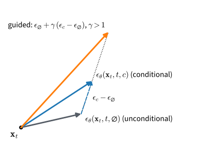
The function evaluates the conditional and unconditional predictions in one batched forward pass, combines them with Equation 17.8.1, and takes the reverse step.
@torch.no_grad()
def sample(net, y, gamma, seed=0):
    """Ancestral sampling with classifier-free guidance of scale gamma."""
    torch.manual_seed(seed)
    n, null = len(y), torch.full_like(y, NULL)
    x = torch.randn(n, 1, 28, 28, device=device)
    for t in reversed(range(T)):
        tt = torch.full((n,), t, device=device)
        eps_c, eps_u = net(torch.cat([x, x]), torch.cat([tt, tt]),
                           torch.cat([y, null])).chunk(2)
        eps = eps_u + gamma * (eps_c - eps_u)
        mean = (x - beta[t] / (1 - alpha_bar[t]).sqrt() * eps) / alpha[t].sqrt()
        x = mean + (beta[t].sqrt() * torch.randn_like(x) if t > 0 else 0)
    return x

def show(imgs, rows, cols):
    imgs = imgs.clamp(-1, 1) / 2 + 0.5
    d2l.show_images(imgs.permute(0, 2, 3, 1).repeat(1, 1, 1, 3), rows, cols,
                    scale=0.8)
@nnx.jit
def guided_step(net, x, t, y, gamma, key):
n = len(y)
tt, null = jnp.full((n,), t), jnp.full((n,), NULL)
eps = net(jnp.concatenate([x, x]), jnp.concatenate([tt, tt]),
jnp.concatenate([y, null]))
eps_c, eps_u = eps[:n], eps[n:] # conditional and unconditional halves
eps = eps_u + gamma * (eps_c - eps_u)
mean = (x - beta[t] / jnp.sqrt(1 - alpha_bar[t]) * eps) / jnp.sqrt(alpha[t])
return mean + jnp.where(t > 0, jnp.sqrt(beta[t]), 0.0) * jax.random.normal(
key, x.shape)
def sample(net, y, gamma, seed=0):
"""Ancestral sampling with classifier-free guidance of scale gamma."""
key = jax.random.PRNGKey(seed)
key, subkey = jax.random.split(key)
x = jax.random.normal(subkey, (len(y), 28, 28, 1))
for t in reversed(range(T)):
key, subkey = jax.random.split(key)
x = guided_step(net, x, t, y, gamma, subkey)
return x
def show(imgs, rows, cols):
imgs = imgs.clip(-1, 1) / 2 + 0.5
d2l.show_images(jnp.repeat(imgs, 3, -1), rows, cols, scale=0.8)17.8.3.1 Unconditional Samples
With \(\gamma = 0\) the label plays no role. Forty-eight samples, each the result of a thousand reverse steps from Gaussian noise with the averaged weights, take one to two minutes.
samples = sample(ema, torch.full((48,), NULL, device=device), gamma=0.0)
show(samples, 6, 8)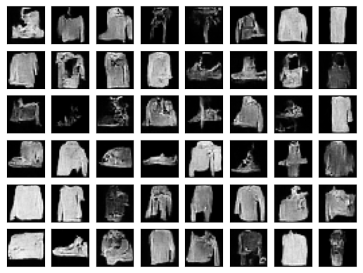
samples = sample(ema, jnp.full((48,), NULL), gamma=0.0)
show(samples, 6, 8)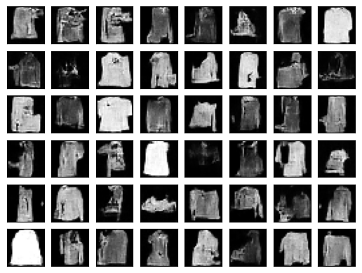
Many of the samples are recognizable garments and shoes, generated by a network of about 340 thousand parameters trained for 1500 updates. Many others are malformed, with uneven outlines, coarse textures, or shapes that mix several classes, a consequence of that budget. The CIFAR-10 model of Ho et al. (2020) has 35.7 million parameters, about a hundred times as many, and trained for 800 thousand updates.
17.8.3.2 Guided Samples
The guidance experiment requests eight samples of every class at three guidance scales. The field measures the fidelity and diversity of samples with feature-space statistics such as the FID and precision–recall of Section 16.5, which need a pretrained feature network and thousands of samples; for \(28 \times 28\) images from a ten-minute model, two direct proxies serve. To measure what guidance does, we train a small convolutional classifier on the clean training images, which reaches close to ninety percent test accuracy in seconds, and use it to score the samples. This classifier only measures the samples; it plays no part in sampling, unlike the noise-trained classifier of classifier guidance. Samples are clamped to \([-1, 1]\), the range of the training images, before they are scored. The three guided runs take several minutes. Two quantities are reported per scale: the fraction of samples that the classifier assigns to the requested class, a proxy for class fidelity, and the mean Euclidean distance between pairs of samples of the same class, a proxy for diversity.
torch.manual_seed(1)
classifier = nn.Sequential(nn.Conv2d(1, 32, 3, 2, 1), nn.ReLU(),
                           nn.Conv2d(32, 64, 3, 2, 1), nn.ReLU(), nn.Flatten(),
                           nn.Linear(64 * 49, 128), nn.ReLU(),
                           nn.Linear(128, 10)).to(device)
optimizer = torch.optim.Adam(classifier.parameters(), lr=1e-3)
for step in range(1000):
    idx = torch.randint(0, len(X), (128,), device=device)
    loss = nn.functional.cross_entropy(classifier(X[idx]), Y[idx])
    optimizer.zero_grad(), loss.backward(), optimizer.step()
with torch.no_grad():
    acc = (classifier(X_test).argmax(1) == Y_test).float().mean()
print(f'classifier test accuracy: {acc:.3f}')
classifier test accuracy: 0.887class Classifier(nnx.Module):
def __init__(self, rngs):
self.c1 = nnx.Conv(1, 32, (3, 3), strides=2, padding='SAME', rngs=rngs)
self.c2 = nnx.Conv(32, 64, (3, 3), strides=2, padding='SAME', rngs=rngs)
self.l1 = nnx.Linear(64 * 49, 128, rngs=rngs)
self.l2 = nnx.Linear(128, 10, rngs=rngs)
def __call__(self, x):
h = nnx.relu(self.c2(nnx.relu(self.c1(x)))).reshape(len(x), -1)
return self.l2(nnx.relu(self.l1(h)))
classifier = Classifier(nnx.Rngs(1))
optimizer = nnx.Optimizer(classifier, optax.adam(1e-3), wrt=nnx.Param)
@nnx.jit
def classifier_step(classifier, optimizer, x, y):
loss_fn = lambda m: optax.softmax_cross_entropy_with_integer_labels(
m(x), y).mean()
loss, grads = nnx.value_and_grad(loss_fn)(classifier)
optimizer.update(classifier, grads)
return loss
for step in range(1000):
key, subkey = jax.random.split(key)
idx = jax.random.randint(subkey, (128,), 0, len(X))
classifier_step(classifier, optimizer, X[idx], Y[idx])
acc = (classifier(X_test).argmax(1) == Y_test).mean()
print(f'classifier test accuracy: {acc:.3f}')classifier test accuracy: 0.893y = torch.arange(10, device=device).repeat(8) # eight samples per class
guided = {}
print(f'{"gamma":>5} {"class agreement":>16} {"within-class distance":>22}')
for gamma in (1.0, 2.0, 4.0):
guided[gamma] = sample(ema, y, gamma, seed=2).clamp(-1, 1)
with torch.no_grad():
agree = (classifier(guided[gamma]).argmax(1) == y).float().mean()
flat = guided[gamma].flatten(1)
dist = torch.stack([torch.pdist(flat[y == c]).mean() for c in range(10)]).mean()
print(f'{gamma:>5.1f} {agree:>16.3f} {dist:>22.2f}')gamma class agreement within-class distance
1.0 0.625 16.63
2.0 0.875 15.33
4.0 0.950 13.44y = jnp.tile(jnp.arange(10), 8) # eight samples per class
guided = {}
print(f'{"gamma":>5} {"class agreement":>16} {"within-class distance":>22}')
for gamma in (1.0, 2.0, 4.0):
guided[gamma] = sample(ema, y, gamma, seed=2).clip(-1, 1)
agree = (classifier(guided[gamma]).argmax(1) == y).mean()
flat = guided[gamma].reshape(80, -1)
dist = jnp.mean(jnp.array([
jnp.linalg.norm(flat[y == c][:, None] - flat[y == c][None], axis=-1).sum()
/ 56 for c in range(10)])) # 8 samples: 56 ordered pairs per class
print(f'{gamma:>5.1f} {agree:>16.3f} {dist:>22.2f}')gamma class agreement within-class distance
1.0 0.650 16.46
2.0 0.850 15.24
4.0 0.875 14.47print('first grid: guidance scale 1; second grid: guidance scale 4; '
'columns are the ten classes')
for gamma in (1.0, 4.0):
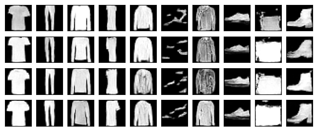
show(guided[gamma][:40], 4, 10) # the first four samples of each classfirst grid: guidance scale 1; second grid: guidance scale 4; columns are the ten classes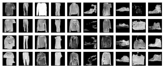
print('first grid: guidance scale 1; second grid: guidance scale 4; '
      'columns are the ten classes')
for gamma in (1.0, 4.0):
    show(guided[gamma][:40], 4, 10)  # the first four samples of each class
first grid: guidance scale 1; second grid: guidance scale 4; columns are the ten classes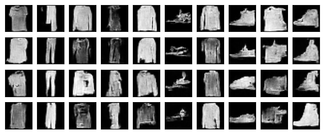
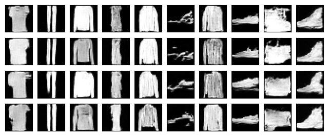
Class agreement rises with the guidance scale and within-class distance falls: stronger guidance produces samples that the classifier assigns to the requested class more reliably and that resemble one another more. The grids, which show the first four samples of each class, show the same effect. At \(\gamma = 1\) each column contains varied instances of its class, some ambiguous; at \(\gamma = 4\) the instances are cleaner and more prototypical, and closer to one another. The cost is visible too: at \(\gamma = 4\) several samples saturate to white, and the sandal column improves little. The trade-off is the one that Ho and Salimans (2022) report on ImageNet, where guidance improves fidelity metrics at the cost of diversity, so the guidance scale is a setting chosen for each application rather than a constant fixed by the derivation.
17.8.3.3 Classifier Guidance
Classifier-free guidance obtains the class direction from the diffusion network itself. The older route, classifier guidance (Dhariwal and Nichol 2021), obtains it from a separate classifier and asks nothing of the diffusion model beyond an unconditional prediction. Written for the noise prediction, the Bayes-rule identity Equation 17.6.3 becomes
\[ \hat{\boldsymbol{\epsilon}}(\mathbf{x}_t, t, c) = \boldsymbol{\epsilon}_{\boldsymbol{\theta}}(\mathbf{x}_t, t, \varnothing) - s\, \sqrt{1 - \bar{\alpha}_t}\; \nabla_{\mathbf{x}_t} \log p_{\boldsymbol{\phi}}(c \mid \mathbf{x}_t, t), \tag{17.8.2}\]
where \(p_{\boldsymbol{\phi}}\) is a classifier of noisy images that takes the step \(t\) as an input, and the scale \(s\) plays the role of \(\gamma\): \(s = 1\) would sample from the Bayes-rule conditional if \(p_{\boldsymbol{\phi}}\) were the exact class posterior of the noisy images, and \(s > 1\) sharpens it. The factor \(\sqrt{1 - \bar{\alpha}_t}\) converts the score-space gradient into the noise-prediction convention of 1. The classifier must be trained on noisy images because its gradient is taken at \(\mathbf{x}_t\), an image at noise level \(t\); a classifier trained only on clean images never saw such inputs, so its gradient there does not estimate \(\nabla_{\mathbf{x}_t} \log p_t(c \mid \mathbf{x}_t)\). The cell trains such a classifier, the architecture of the classifier above with a second input channel that carries the noise level \(\sqrt{1 - \bar{\alpha}_t}\), on noisy training images at random steps, and reports its accuracy on clean test images and on test images at the middle of the schedule.
class NoisyClassifier(nn.Module):
    """A classifier of noisy images; the noise level enters as a second channel."""
    def __init__(self):
        super().__init__()
        self.net = nn.Sequential(nn.Conv2d(2, 32, 3, 2, 1), nn.ReLU(),
                                 nn.Conv2d(32, 64, 3, 2, 1), nn.ReLU(), nn.Flatten(),
                                 nn.Linear(64 * 49, 128), nn.ReLU(), nn.Linear(128, 10))

    def forward(self, x, t):
        level = (1 - alpha_bar[t]).sqrt()[:, None, None, None].expand_as(x)
        return self.net(torch.cat([x, level], 1))

torch.manual_seed(3)
noisy_classifier = NoisyClassifier().to(device)
optimizer = torch.optim.Adam(noisy_classifier.parameters(), lr=1e-3)
for step in range(2000):
    idx = torch.randint(0, len(X), (128,), device=device)
    x0, y_batch = X[idx], Y[idx]
    t = torch.randint(0, T, (128,), device=device)
    a = alpha_bar[t][:, None, None, None]
    x_t = a.sqrt() * x0 + (1 - a).sqrt() * torch.randn_like(x0)
    loss = nn.functional.cross_entropy(noisy_classifier(x_t, t), y_batch)
    optimizer.zero_grad(), loss.backward(), optimizer.step()
with torch.no_grad():
    t_mid = torch.full((len(X_test),), T // 2, device=device)
    a = alpha_bar[t_mid][:, None, None, None]
    x_mid = a.sqrt() * X_test + (1 - a).sqrt() * torch.randn_like(X_test)
    t_clean = torch.zeros(len(X_test), dtype=torch.long, device=device)
    acc_clean = (noisy_classifier(X_test, t_clean).argmax(1) == Y_test).float().mean()
    acc_mid = (noisy_classifier(x_mid, t_mid).argmax(1) == Y_test).float().mean()
print(f'noisy classifier test accuracy: {acc_clean:.3f} at t = 0, '
      f'{acc_mid:.3f} at t = {T // 2}')
noisy classifier test accuracy: 0.853 at t = 0, 0.600 at t = 500class NoisyClassifier(nnx.Module):
"""A classifier of noisy images; the noise level enters as a second channel."""
def __init__(self, rngs):
self.c1 = nnx.Conv(2, 32, (3, 3), strides=2, padding='SAME', rngs=rngs)
self.c2 = nnx.Conv(32, 64, (3, 3), strides=2, padding='SAME', rngs=rngs)
self.l1 = nnx.Linear(64 * 49, 128, rngs=rngs)
self.l2 = nnx.Linear(128, 10, rngs=rngs)
def __call__(self, x, t):
level = jnp.sqrt(1 - alpha_bar[t])[:, None, None, None]
h = jnp.concatenate([x, jnp.broadcast_to(level, x.shape)], -1)
h = nnx.relu(self.c2(nnx.relu(self.c1(h)))).reshape(len(x), -1)
return self.l2(nnx.relu(self.l1(h)))
noisy_classifier = NoisyClassifier(nnx.Rngs(3))
optimizer = nnx.Optimizer(noisy_classifier, optax.adam(1e-3), wrt=nnx.Param)
@nnx.jit
def noisy_classifier_step(classifier, optimizer, x0, y, t, eps):
def loss_fn(model):
a = alpha_bar[t][:, None, None, None]
logits = model(jnp.sqrt(a) * x0 + jnp.sqrt(1 - a) * eps, t)
return optax.softmax_cross_entropy_with_integer_labels(logits, y).mean()
loss, grads = nnx.value_and_grad(loss_fn)(classifier)
optimizer.update(classifier, grads)
return loss
for step in range(2000):
key, k1, k2, k3 = jax.random.split(key, 4)
idx = jax.random.randint(k1, (128,), 0, len(X))
noisy_classifier_step(noisy_classifier, optimizer, X[idx], Y[idx],
jax.random.randint(k2, (128,), 0, T),
jax.random.normal(k3, (128, 28, 28, 1)))
key, subkey = jax.random.split(key)
t_mid = jnp.full((len(X_test),), T // 2)
a = alpha_bar[t_mid][:, None, None, None]
x_mid = jnp.sqrt(a) * X_test + jnp.sqrt(1 - a) * jax.random.normal(subkey, X_test.shape)
t_clean = jnp.zeros(len(X_test), jnp.int32)
acc_clean = (noisy_classifier(X_test, t_clean).argmax(1) == Y_test).mean()
acc_mid = (noisy_classifier(x_mid, t_mid).argmax(1) == Y_test).mean()
print(f'noisy classifier test accuracy: {acc_clean:.3f} at t = 0, '
f'{acc_mid:.3f} at t = {T // 2}')noisy classifier test accuracy: 0.848 at t = 0, 0.581 at t = 500The sampler is the ancestral chain of sample with Equation 17.8.2 in place of the classifier-free rule: at each step it takes the unconditional prediction of the same U-Net, computes the gradient of the classifier’s log-probability of the requested class with respect to the current noisy image by automatic differentiation, and combines the two. We run it for the same eighty requests at three scales and score the samples with the clean classifier as before, so that both rules are scored the same way.
def classifier_gradient(classifier, x, t, y):
    """Gradient of log p(y | x_t) with respect to x_t for every image in the batch."""
    x = x.detach().requires_grad_(True)
    log_prob = torch.log_softmax(classifier(x, t), 1).gather(1, y[:, None]).sum()
    return torch.autograd.grad(log_prob, x)[0]

def sample_classifier_guided(net, classifier, y, scale, seed=0):
    """Ancestral sampling with classifier guidance of scale `scale`."""
    torch.manual_seed(seed)
    n, null = len(y), torch.full_like(y, NULL)
    x = torch.randn(n, 1, 28, 28, device=device)
    for t in reversed(range(T)):
        tt = torch.full((n,), t, device=device)
        with torch.no_grad():
            eps = net(x, tt, null)  # the unconditional prediction
        eps = eps - scale * (1 - alpha_bar[t]).sqrt() * classifier_gradient(
            classifier, x, tt, y)
        with torch.no_grad():
            mean = (x - beta[t] / (1 - alpha_bar[t]).sqrt() * eps) / alpha[t].sqrt()
            x = mean + (beta[t].sqrt() * torch.randn_like(x) if t > 0 else 0)
    return x

classifier_guided = {}
print(f'{"scale":>5} {"class agreement":>16} {"within-class distance":>22}')
for scale in (1.0, 4.0, 10.0):
    classifier_guided[scale] = sample_classifier_guided(
        ema, noisy_classifier, y, scale, seed=2).clamp(-1, 1)
    with torch.no_grad():
        agree = (classifier(classifier_guided[scale]).argmax(1) == y).float().mean()
    flat = classifier_guided[scale].flatten(1)
    dist = torch.stack([torch.pdist(flat[y == c]).mean() for c in range(10)]).mean()
    print(f'{scale:>5.1f} {agree:>16.3f} {dist:>22.2f}')
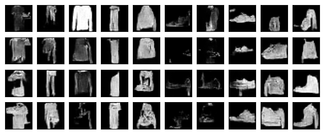
print('first grid: scale 1; second grid: scale 10; columns are the ten classes')
for scale in (1.0, 10.0):
    show(classifier_guided[scale][:40], 4, 10)
scale class agreement within-class distance
1.0 0.488 18.54
4.0 0.788 16.12
10.0 0.838 15.19
first grid: scale 1; second grid: scale 10; columns are the ten classes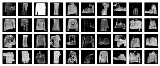
@nnx.jit
def classifier_guided_step(net, classifier, x, t, y, scale, key):
    n = len(y)
    tt, null = jnp.full((n,), t), jnp.full((n,), NULL)
    eps = net(x, tt, null)  # the unconditional prediction
    log_prob = lambda x: jnp.take_along_axis(  # sum of log p(y_i | x_i), one term per image
        jax.nn.log_softmax(classifier(x, tt), 1), y[:, None], 1).sum()
    eps = eps - scale * jnp.sqrt(1 - alpha_bar[t]) * jax.grad(log_prob)(x)
    mean = (x - beta[t] / jnp.sqrt(1 - alpha_bar[t]) * eps) / jnp.sqrt(alpha[t])
    return mean + jnp.where(t > 0, jnp.sqrt(beta[t]), 0.0) * jax.random.normal(
        key, x.shape)

def sample_classifier_guided(net, classifier, y, scale, seed=0):
    """Ancestral sampling with classifier guidance of scale `scale`."""
    key = jax.random.PRNGKey(seed)
    key, subkey = jax.random.split(key)
    x = jax.random.normal(subkey, (len(y), 28, 28, 1))
    for t in reversed(range(T)):
        key, subkey = jax.random.split(key)
        x = classifier_guided_step(net, classifier, x, t, y, scale, subkey)
    return x

classifier_guided = {}
print(f'{"scale":>5} {"class agreement":>16} {"within-class distance":>22}')
for scale in (1.0, 4.0, 10.0):
    classifier_guided[scale] = sample_classifier_guided(
        ema, noisy_classifier, y, scale, seed=2).clip(-1, 1)
    agree = (classifier(classifier_guided[scale]).argmax(1) == y).mean()
    flat = classifier_guided[scale].reshape(80, -1)
    dist = jnp.mean(jnp.array([
        jnp.linalg.norm(flat[y == c][:, None] - flat[y == c][None], axis=-1).sum()
        / 56 for c in range(10)]))  # 8 samples: 56 ordered pairs per class
    print(f'{scale:>5.1f} {agree:>16.3f} {dist:>22.2f}')
print('first grid: scale 1; second grid: scale 10; columns are the ten classes')
for scale in (1.0, 10.0):
    show(classifier_guided[scale][:40], 4, 10)
scale class agreement within-class distance
1.0 0.512 18.33
4.0 0.812 16.65
10.0 0.900 15.96
first grid: scale 1; second grid: scale 10; columns are the ten classes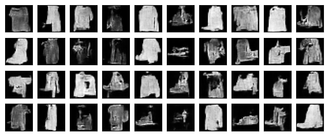
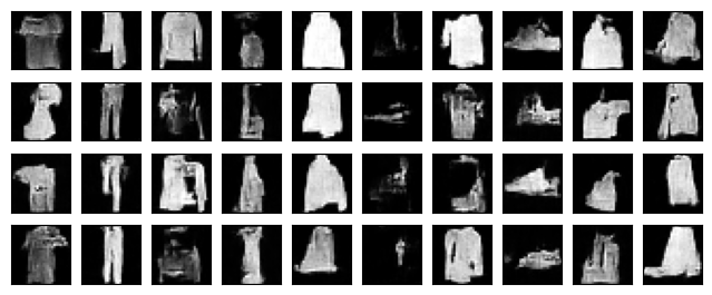
The noisy classifier is a few points less accurate than the clean one on clean images and still right more often than not halfway through the schedule. With the scale at one, which targets the Bayes-rule conditional, classifier guidance steers only weakly: about half of the samples land in the requested class, fewer than under classifier-free guidance at \(\gamma = 1\). Dhariwal and Nichol (2021) report a similar weakness on ImageNet: at scale one their samples did not match the requested classes on inspection, although their guiding classifier gave those classes about fifty percent probability; larger scales remedied this. Raising the scale raises agreement and lowers within-class distance, as before; at a scale of ten the agreement matches that of classifier-free guidance at \(\gamma = 4\), while the within-class distance stays larger. The grids temper this comparison: at scale ten, more samples are malformed or faint than under classifier-free guidance at \(\gamma = 4\). Classifier guidance ascends the log-probability of a classifier with the same architecture and training data as the one that scores the samples, so it can raise agreement without producing a recognizable garment, and pixel distance grows with such artifacts as well as with diversity; Ho and Salimans (2022) raise the same concern about classifier-based metrics. The other cost is a second network, trained on noisy images, that steers toward whatever it has learned, including its confusions between similar garments. Ho and Salimans (2022) introduced the classifier-free rule to remove that network, and with it the need for a classifier of noisy data.
17.8.4 Outlook
The model trained here has the structure of the systems that generate images from text, and the differences are matters of scale and of a few later ideas, two of which the next sections develop. Sampling with a thousand network evaluations is the main cost, and Section 17.9 shows that a trained noise predictor also supports a deterministic sampler, which for a well-trained network needs only a few dozen evaluations (J. Song et al. 2021). Section 17.10 replaces the noise predictor by a velocity field regressed on straight noise-to-data segments, the formulation that Esser et al. (2024) scale to large text-to-image models, and shows how the two views are related. Section 17.11 then extends the construction to categorical data such as text.
Four further lines of work act on different parts of the model.
On the sampler, improved schedules and learned reverse variances (Nichol and Dhariwal 2021) and a careful redesign of the noise parameterization and sampler (Karras et al. 2022) reduce the step count further, and distillation trains a student to reproduce the sampler’s output in one to four evaluations (Salimans and Ho 2022; Song et al. 2023); a later line of distillation adds an adversarial loss to the student (Sauer et al. 2023), which is where adversarial training re-enters (Section 16.7).
On the data space, latent diffusion (Rombach et al. 2022) runs the diffusion in the latent space of an autoencoder, so that its U-Net, itself hundreds of millions of parameters or more, operates on a compressed image, and the decoder maps each generated latent back to an image in a single pass. Sampling in the smaller space is much cheaper, but the images are limited by what the autoencoder preserves: Rombach et al. (2022) find that too strong a compression limits the achievable quality and too weak a compression slows training. The model conditions on text through cross-attention layers inside the U-Net that attend to the token embeddings of a text encoder, a richer injection than the single vector added to the time embedding here.
On the backbone, transformers replace the U-Net at the largest scales (Peebles and Xie 2023).
On the objective and the theory, the variational bound of Section 17.7 also makes diffusion models competitive likelihood estimators when trained on it rather than on the simple loss (Kingma et al. 2021), and the continuous-time view of Section 29.4 places the ladder, the chain, and the samplers of this chapter in one framework: the ladder and the chain discretize the variance-exploding and the variance-preserving stochastic differential equations, the ancestral sampler discretizes the reverse-time equation, and the deterministic sampler of Section 17.9 its probability-flow equation (Y. Song et al. 2021); Lai et al. (2025) develop that view in full.
17.8.5 Summary
A class-conditional diffusion model for images is the model of Section 17.7 with a U-Net as the noise predictor, a class embedding added to the time embedding, and a null label that makes the same network unconditional. Trained by the simple loss with label dropout, and sampled with an exponential moving average of the weights, a network of about 340 thousand parameters produces Fashion-MNIST samples, many of them recognizable, after ten minutes of laptop training.
Classifier-free guidance combines the two predictions the network provides: the guided noise prediction extrapolates from the unconditional prediction through the conditional one by a scale \(\gamma\). Increasing \(\gamma\) raised the fraction of samples that a classifier assigned to the requested class and lowered the pixel distance between samples of the same class. These are the proxies used here for fidelity and diversity, and the scale sets the trade-off between them. Classifier guidance, which draws the class direction from a separate classifier trained on noisy images, raised agreement and lowered within-class distance in the same way on the same requests, at the cost of that second network and with more malformed samples at the largest scale. Fast samplers, latent-space diffusion, larger backbones, and the continuous-time formulation build on the model of this chapter rather than replacing it.
17.8.6 Exercises
- Guidance in score space. Starting from Bayes’ rule at noise level \(t\), derive Equation 17.8.1 in two steps: express \(\nabla \log p_t(c \mid \mathbf{x})\) through the conditional and unconditional scores, then convert scores to noise predictions using
- Show that \(\gamma = 1\) recovers the conditional prediction exactly and that, for \(\gamma \neq 1\), the guided field is the score of \(p_t(\mathbf{x}) \, p_t(c \mid \mathbf{x})^\gamma\) up to normalization.
- The null label. Suppose label dropout were omitted, so that the network never saw the null label during training. Which of the quantities in Equation 17.8.1 would be untrained, and what would the sampler compute at \(\gamma = 0\)? Then explain why a dropout probability near one would also be harmful.
- [code] The moving average. Sample forty-eight images with the raw weights
netinstead ofema, using the same seed, and compare the two grids. Then repeat the training with the decay held at \(0.999\) from the first step, and explain what you observe in the averaged model’s samples in terms of the warm-up. - [code] Guidance scales. Extend the guidance experiment to \(\gamma \in \{0.5, 1, 2, 4, 8, 16\}\) and plot class agreement and within-class distance against \(\gamma\). Describe what happens to the samples at the largest scales, and relate it to the caveat that the guided field is in general not the score of a noised data distribution.
- [code] Fewer sampling steps. Modify
sampleto use every tenth step of the schedule, merging the skipped steps as in Exercise 6 of Section 17.7, and compare the samples and the classifier agreement with the full thousand-step sampler. How many steps can be removed before the samples degrade visibly? - [code] Inpainting. Take a test image, mask its lower half, and generate the missing half by ancestral sampling in which, after every reverse step, the known pixels are replaced by a noised copy of the original at the current step (drawn from Equation 17.7.2). Show the results for several images and explain why the replacement uses the noised original rather than the clean one.