%matplotlib inline
from d2l import torch as d2l
import torch10.1 Queries, Keys, and Values
Many neural networks either assume a fixed input size or compress a variable-length input into a fixed-dimensional state. RNNs (Section 8.4) and specialized convolutions (Kalchbrenner et al. 2014) can process variable-length sequences, but their fixed-size summaries may lose information in long sequences. We seek an operation that can access any input representation while using a fixed set of parameters.
Databases have this property because a query is evaluated against stored key–value pairs. Consider the scalar database \(\mathcal{D}=\{(2,10),(5,20)\}\). An exact query \(q=5\) returns the value 20. A soft query first defines a score, for example \(a(q,k)=-(q-k)^2\), and normalizes the two scores. For \(q=4\), key 5 receives the larger weight, but both values contribute to the result. The same rule works for any database size, and its output changes when the stored pairs change; the query does not require compressing the database into one fixed vector first.
The attention mechanism (Bahdanau et al. 2015) is a differentiable version of this lookup. This section defines the operation and illustrates it with classical kernel regression, where the attention weights are specified by a kernel rather than learned.
%matplotlib inline
from d2l import jax as d2l
import jax
from jax import numpy as jnp
10.1.1 Attention as Differentiable Lookup
Let \(\mathbf{q},\mathbf{k}_i \in \mathbb{R}^{d_k}\) and \(\mathbf{v}_i \in \mathbb{R}^{d_v}\). Denote by \(\mathcal{D} \stackrel{\textrm{def}}{=} \{(\mathbf{k}_1, \mathbf{v}_1), \ldots, (\mathbf{k}_m, \mathbf{v}_m)\}\) a database of \(m\) key–value pairs. We define the attention output in \(\mathbb{R}^{d_v}\) by
\[\textrm{Attention}(\mathbf{q}, \mathcal{D}) \stackrel{\textrm{def}}{=} \sum_{i=1}^m \alpha(\mathbf{q}, \mathbf{k}_i) \mathbf{v}_i, \tag{10.1.1}\]
where the scalar weights \(\alpha(\mathbf{q},\mathbf{k}_i)\) determine each value’s contribution. In the layers used below, the weights are nonnegative and sum to one, so the output is a convex combination of the values. Exact lookup is the limiting one-hot case, and uniform weights give average pooling. Signed or unnormalized variants exist, but they are not the default operation in this chapter.
A common strategy for ensuring that the weights sum up to \(1\) is to start from any scoring function \(a(\mathbf{q}, \mathbf{k})\) and normalize. To make the weights nonnegative as well, we exponentiate first. This means we can pick any function \(a(\mathbf{q}, \mathbf{k})\) and apply the softmax operation known from multinomial models:
\[\alpha(\mathbf{q}, \mathbf{k}_i) = \frac{\exp(a(\mathbf{q}, \mathbf{k}_i))}{\sum_j \exp(a(\mathbf{q}, \mathbf{k}_j))}. \tag{10.1.2}\]
This operation is available in all deep learning frameworks and is differentiable. For at least two entries and finite scores, its Jacobian is not the zero matrix, although its entries can become very small when the distribution saturates. Nondifferentiable attention mechanisms also exist and may be trained with reinforcement learning (Mnih et al. 2014), but they are harder to optimize. This chapter uses the differentiable framework in Figure 10.1.1.
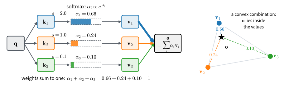
The query and compatibility function use a fixed number of parameters even when the number of key–value pairs changes. Attention pooling can therefore operate on inputs of different lengths without first compressing them to a fixed-size state.
10.1.2 Visualizing Attention Weights
When the weights are nonnegative and sum to \(1\), we may interpret large weights as the model selecting the components that matter for the query at hand. This is a useful intuition, though only an intuition—we return to how much attention weights actually explain at the end of the chapter. Either way, plotting the weight matrix over (query, key) pairs is the standard diagnostic, and we will use it throughout the chapter via the d2l.show_heatmaps helper. It accepts a tensor of shape (number of rows for display, number of columns for display, number of queries, number of keys), so a whole grid of weight matrices can be compared side by side.
As a sanity check, we visualize the identity matrix, which represents the exact-lookup case: the attention weight is \(1\) exactly when query and key agree.
attention_weights = torch.eye(10).reshape((1, 1, 10, 10))
d2l.show_heatmaps(attention_weights, xlabel='Keys', ylabel='Queries')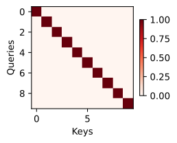
attention_weights = jnp.eye(10).reshape((1, 1, 10, 10))
d2l.show_heatmaps(attention_weights, xlabel='Keys', ylabel='Queries')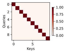
10.1.3 Attention Pooling with Fixed Kernels
Equation Equation 10.1.1 does not require learned weights. Long before deep learning, statisticians used this operation with specified weights: Nadaraya–Watson kernel regression (Nadaraya 1964; Watson 1964). This classical setting makes the effect of the weights visible on a problem we can plot. Its fixed similarity function also motivates the learned scoring rules developed in the rest of the chapter.
10.1.3.1 Similarity Kernels
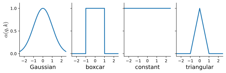
A kernel \(\alpha(\mathbf{q}, \mathbf{k})\) measures the similarity between a query and a key, typically as a decreasing function of their distance. Common choices include
\[ \begin{aligned} \alpha(\mathbf{q}, \mathbf{k}) & = \exp\left(-\tfrac{1}{2} \|\mathbf{q} - \mathbf{k}\|^2 \right) && \textrm{Gaussian;} \\ \alpha(\mathbf{q}, \mathbf{k}) & = 1 \textrm{ if } \|\mathbf{q} - \mathbf{k}\| \leq 1 && \textrm{boxcar;} \\ \alpha(\mathbf{q}, \mathbf{k}) & = \mathop{\mathrm{max}}\left(0, 1 - \|\mathbf{q} - \mathbf{k}\|\right) && \textrm{triangular,} \end{aligned} \tag{10.1.3}\]
plus the degenerate constant kernel \(\alpha(\mathbf{q}, \mathbf{k}) = 1\) that ignores the query entirely. Figure 10.1.2 shows their shapes; many more exist, and the choice of kernel connects to kernel density estimation, also known as Parzen windows (Parzen 1957).
Normalizing any such kernel over the keys, as in Equation 10.1.2 but without the exponentiation (the kernels are already nonnegative), yields the Nadaraya–Watson estimator
\[f(\mathbf{q}) = \sum_i \mathbf{v}_i \frac{\alpha(\mathbf{q}, \mathbf{k}_i)}{\sum_j \alpha(\mathbf{q}, \mathbf{k}_j)}. \tag{10.1.4}\]
For scalar regression with observations \((x_i, y_i)\), the keys are the training inputs \(x_i\), the values are the labels \(y_i\), and the query is the location where we want an estimate. Equation Equation 10.1.4 is attention pooling, term for term. The estimator needs no training at all, and if the kernel is narrowed at a suitable rate as data accumulates, it converges to the statistically optimal predictor (Mack and Silverman 1982).
10.1.3.2 Nadaraya–Watson Regression in Action
To examine the estimator, we draw \(40\) noisy training examples from \(y = 2\sin(x) + x + \epsilon\) with standard Gaussian noise \(\epsilon\) and evaluate on a grid.
torch.manual_seed(0)
n = 40
x_train, _ = torch.sort(torch.rand(n) * 5)
y_train = 2 * torch.sin(x_train) + x_train + torch.randn(n)
x_val = torch.arange(0, 5, 0.1)
y_val = 2 * torch.sin(x_val) + x_val
key1, key2 = jax.random.split(jax.random.key(0))
n = 40
x_train = jnp.sort(jax.random.uniform(key1, (n,)) * 5)
y_train = 2 * jnp.sin(x_train) + x_train + jax.random.normal(key2, (n,))
x_val = jnp.arange(0, 5, 0.1)
y_val = 2 * jnp.sin(x_val) + x_valThe estimator itself is four lines: compute all query–key distances, apply a Gaussian kernel with bandwidth \(\sigma\), normalize over the keys, and take the weighted sum of the values. The normalized kernel matrix is the attention weight matrix, so we return it too. For these data, the bandwidth affects the estimate more than the choice among the displayed kernel shapes. We therefore vary \(\sigma\) and keep the kernel Gaussian.
def nadaraya_watson(x_train, y_train, x_val, sigma):
    dists = x_train[:, None] - x_val[None, :]
    k = torch.exp(-dists**2 / (2 * sigma**2))
    attention_w = k / k.sum(0)  # Normalize over keys for each query
    return y_train @ attention_w, attention_w

sigmas = (0.1, 0.5, 2.0)
estimates = [nadaraya_watson(x_train, y_train, x_val, s)[0] for s in sigmas]
d2l.plot(x_val, estimates + [y_val], 'x', 'y',
         legend=[f'sigma = {s:g}' for s in sigmas] + ['truth'])
d2l.plt.plot(x_train, y_train, 'o', alpha=0.4);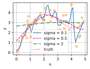
def nadaraya_watson(x_train, y_train, x_val, sigma):
    dists = x_train[:, None] - x_val[None, :]
    k = jnp.exp(-dists**2 / (2 * sigma**2))
    attention_w = k / k.sum(0)  # Normalize over keys for each query
    return y_train @ attention_w, attention_w

sigmas = (0.1, 0.5, 2.0)
estimates = [nadaraya_watson(x_train, y_train, x_val, s)[0] for s in sigmas]
d2l.plot(x_val, estimates + [y_val], 'x', 'y',
         legend=[f'sigma = {s:g}' for s in sigmas] + ['truth'])
d2l.plt.plot(x_train, y_train, 'o', alpha=0.4);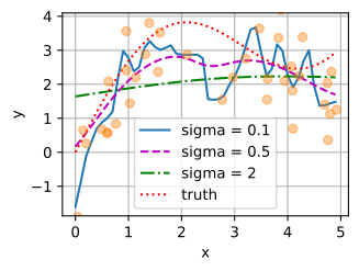
All three bandwidths produce workable estimates. The narrow kernel chases individual noisy observations; the wide one oversmooths toward a global average; \(\sigma = 0.5\) tracks the underlying function well. The attention weights show how the bandwidth produces these differences:
_, w_narrow = nadaraya_watson(x_train, y_train, x_val, 0.1)
_, w_wide = nadaraya_watson(x_train, y_train, x_val, 2.0)
d2l.show_heatmaps(torch.stack([w_narrow.T, w_wide.T])[None],
                  xlabel='Training inputs (keys)',
                  ylabel='Test inputs (queries)',
                  titles=['sigma = 0.1', 'sigma = 2'], figsize=(7, 3))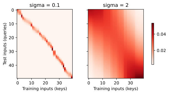
_, w_narrow = nadaraya_watson(x_train, y_train, x_val, 0.1)
_, w_wide = nadaraya_watson(x_train, y_train, x_val, 2.0)
d2l.show_heatmaps(jnp.stack([w_narrow.T, w_wide.T])[None],
                  xlabel='Training inputs (keys)',
                  ylabel='Test inputs (queries)',
                  titles=['sigma = 0.1', 'sigma = 2'], figsize=(7, 3))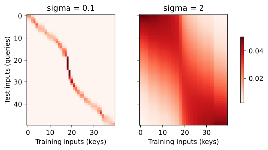
The narrow kernel concentrates each query’s weight on a handful of nearby keys—sharp, local, and noisy—while the wide kernel spreads it across much of the dataset. Picking one global \(\sigma\) is itself a compromise; Silverman (1986) proposed bandwidths that adapt to the local data density, and similar nearest-neighbor interpolation ideas resurface in modern cross-modal representation learning (Norelli et al. 2022).
Nadaraya–Watson regression fixes the kernel shape, bandwidth, and space in which distances are measured. Every query therefore uses the same prescribed notion of similarity. A learned attention mechanism instead learns query and key representations whose induced weights serve the task. The next section develops a learnable scoring function.
10.1.4 Summary
Attention pooling Equation 10.1.1 forms a weighted sum of values, where each weight depends on compatibility between a query and a key. Softmax applied to a scoring function produces nonnegative weights that sum to one. Exact lookup and average pooling are special cases. Nadaraya–Watson regression uses a fixed similarity kernel; modern attention instead learns representations of queries and keys.
10.1.5 Exercises
- A two-entry database. Consider the database \(\mathcal{D} =
\{(2, 10), (5, 20)\}\) of scalar keys and values, with the score \(a(q, k) = -(q - k)^2\) normalized by Equation 10.1.2.
- Compute the two weights and the output for the query \(q = 4\).
- Express the output as a function of \(q\). Which query returns \(15\), and which outputs do the queries \(q \in \mathbb{R}\) reach?
- Replace the score by \(a(q, k) = -(q - k)^2 / (2\sigma^2)\). Describe the output as a function of \(q\) in the limits \(\sigma \to 0\) and \(\sigma \to \infty\), and state which lookup each limit performs.
- A fixed parameter budget. A database holds \(m\) key–value pairs with \(\mathbf{k}_i \in \mathbb{R}^{d_k}\) and \(\mathbf{v}_i \in \mathbb{R}^{d_v}\), and the lookup Equation 10.1.1 scores them with a learned bilinear form \(a(\mathbf{q}, \mathbf{k}) = \mathbf{q}^\top \mathbf{M}
\mathbf{k}\), \(\mathbf{M} \in \mathbb{R}^{d_k \times d_k}\).
- Count the parameters of this lookup and the number of scores it evaluates for one query.
- A fully connected layer instead maps the concatenation of the query and all \(m\) pairs, a vector of length \(d_k + m(d_k + d_v)\), to an output in \(\mathbb{R}^{d_v}\). Count its parameters as a function of \(m\).
- The pairs of a database carry no order. Determine how the output of each of the two maps changes when the \(m\) pairs are permuted.
- An average of two values. Let the keys \(\mathbf{k}_1, \ldots,
\mathbf{k}_m\) be orthonormal and let the score be \(a(\mathbf{q},
\mathbf{k}) = \mathbf{q}^\top \mathbf{k}\) with the weights of
Equation 10.1.2.
- For the query \(\mathbf{q} = c\,(\mathbf{k}_a + \mathbf{k}_b)\) with \(c > 0\), compute all \(m\) weights and show that the output tends to \(\tfrac{1}{2}(\mathbf{v}_a + \mathbf{v}_b)\) as \(c \to \infty\).
- How large must \(c\) be for the two selected keys to receive at least 99% of the total weight when \(m = 10\)?
- Now let the keys be orthogonal with \(\|\mathbf{k}_b\| = 2\,\|\mathbf{k}_a\|\). Find a query that again averages \(\mathbf{v}_a\) and \(\mathbf{v}_b\), and state what \(\mathbf{q} = c\,(\mathbf{k}_a + \mathbf{k}_b)\) returns instead as \(c \to \infty\).
- [code] The gradient of attention. ● Suppose that \(a(\mathbf{q},
\mathbf{k}_i) = \mathbf{q}^\top \mathbf{k}_i\) and that \(\mathbf{k}_i =
\mathbf{v}_i\) for \(i = 1, \ldots, m\). Denote by \(p(\mathbf{k}_i;
\mathbf{q})\) the distribution over keys defined by the softmax normalization Equation 10.1.2.
- Prove that \[\nabla_{\mathbf{q}} \mathop{\textrm{Attention}}(\mathbf{q}, \mathcal{D}) = \textrm{Cov}_{p(\mathbf{k}_i; \mathbf{q})}[\mathbf{k}_i].\]
- Conclude that this Jacobian is positive semidefinite, and determine for which databases it is the zero matrix.
- Let \(\mathbf{q} = c\,\mathbf{u}\) for a fixed direction \(\mathbf{u}\) for which exactly one key attains the largest score \(\mathbf{u}^\top \mathbf{k}_i\). Find the limit of the Jacobian as \(c \to \infty\), and state what it implies for training the query by gradient descent.
- Verify the identity and the limit with automatic differentiation on a random database with \(m = 8\) and \(d_k = 4\).
- [code] Soft lookup as retrieval. ● Build a database of \(m\) keys drawn uniformly from the unit sphere in \(\mathbb{R}^{16}\), with value \(\mathbf{v}_i\) the one-hot indicator of index \(i\), and weight them with the Gaussian kernel of bandwidth \(\sigma\) normalized as in
Equation 10.1.4. A query \(\mathbf{q} = \mathbf{k}_i +
\boldsymbol{\epsilon}\) with \(\boldsymbol{\epsilon} \sim
\mathcal{N}(\mathbf{0}, \tau^2 \mathbf{I})\) is retrieved correctly when the largest entry of the output is entry \(i\).
- Show that the retrieved index is the index of the nearest key for every \(\sigma > 0\), so the bandwidth does not affect which index is retrieved.
- Without noise, the weight on the correct key is \[\alpha_i = \frac{1}{1 + \sum_{j \neq i} \exp\big(-\|\mathbf{k}_i - \mathbf{k}_j\|^2 / 2\sigma^2\big)}. \tag{10.1.5}\] Approximate \(\mathbf{k}_i^\top \mathbf{k}_j \approx 0\) for random unit vectors, so that \(\|\mathbf{k}_i - \mathbf{k}_j\|^2 \approx 2\), and derive the bandwidth at which \(\alpha_i\) falls to \(0.9\) for \(m = 20\) and for \(m = 200\). How must \(\sigma\) shrink as \(m\) grows?
- Measure \(\alpha_i\) at these two bandwidths, averaged over random databases, and explain the direction of its discrepancy from \(0.9\).
- Sweep \(\tau\) from \(0\) to \(1\) at \(m = 20\) and \(m = 200\), with the bandwidth from (b) for each \(m\), and plot the retrieval accuracy against \(\tau\). Compute the weights as the softmax Equation 10.1.2 of the scores \(-\|\mathbf{q} - \mathbf{k}_j\|^2 / 2\sigma^2\). Explain why a larger \(m\) lowers the accuracy at fixed \(\tau\) although the distance from the query to the correct key is unchanged.
- [code] Effective number of keys. For the weights \(\alpha_i(q)\) of one query, define the effective number of keys \(n_{\textrm{eff}}(q) = 1 / \sum_i \alpha_i(q)^2\).
- Show that \(1 \leq n_{\textrm{eff}}(q) \leq m\) for \(m\) nonnegative weights that sum to one, and identify the weights that attain each bound.
- Let the values be \(y_i = g(x_i) + \epsilon_i\) with independent noise of variance \(s^2\), and hold the keys fixed. Show that the variance of the estimate Equation 10.1.4 at \(q\) is \(s^2 / n_{\textrm{eff}}(q)\).
- Compute \(n_{\textrm{eff}}\) at every query in
x_valfrom the weights thatnadaraya_watsonreturns, for each bandwidth insigmas, and plot the three curves. Then redraw the noise iny_train200 times withx_trainfixed, and compare the standard deviation of the estimate at each query with \(1 / \sqrt{n_{\textrm{eff}}(q)}\).
- [code] Boxcar and triangular kernels. The section states that for the data
x_trainandy_trainthe bandwidth affects the estimate more than the choice among the kernel shapes of Equation 10.1.3 does, and then varies only \(\sigma\). Test the claim.- Extend
nadaraya_watsonwith the boxcar and triangular kernels, each with a radius \(h\) in place of the unit distance. Display the weights of the Gaussian kernel at \(\sigma = 0.5\) and of the other two kernels at \(h = 0.5\) side by side withd2l.show_heatmaps, and describe how the rows of the three matrices differ. - Which of the kernels can leave a query with all-zero weights? Count the queries in
x_valthat this affects at \(h = 0.05\), and define the estimate at those queries. - For each kernel, sweep the bandwidth \(\sigma\) or the radius \(h\) over 20 values between \(0.05\) and \(3\), record the mean squared error against
y_val, and plot the three error curves. - Compare the spread of the error across the three kernels at their best bandwidths with the spread across bandwidths for one kernel. Does the comparison support the claim? Redraw the training noise five times. Is the ranking of the kernels at their best bandwidths stable?
- Extend
- [code] Queries beyond the data. The estimate Equation 10.1.4 is a convex combination of the values, and the inputs
x_trainlie in the interval \([0, 5)\).- For distinct scalar keys and a Gaussian kernel of fixed bandwidth, find the limit of the estimate as \(q \to \infty\). Find the same limit for the constant kernel.
- Evaluate
nadaraya_watsonwith \(\sigma = 0.5\) at the queries \(5, 5.5, \ldots, 10\) and plot the estimate against \(y = 2\sin(x) + x\). Explain why no nonnegative kernel and no bandwidth let the estimate follow the trend of the truth. - With \(\sigma = 0.5\),
nadaraya_watsonreturns NaN at the query \(q = 15\). Explain why in single precision, and compute the weights instead as the softmax Equation 10.1.2 of the scores \(-(q - x_i)^2 / (2\sigma^2)\), so that the estimate is finite at every query and every bandwidth.
- [code] A learned bandwidth. Treat \(\sigma\) in
nadaraya_watsonas a parameter and fit it by gradient descent onx_trainandy_train.- Before running, predict the minimizer of the training error \(\sum_i (f(x_i) - y_i)^2\), given that \(y_i\) enters the computation of \(f(x_i)\) through its own kernel weight.
- Run the optimization from \(\sigma = 1\), report where \(\sigma\) goes, and compare the fitted curve with the estimates for the bandwidths in
sigmas. - Exclude \((x_i, y_i)\) from the estimate at \(x_i\) by zeroing the diagonal of the kernel matrix and refit. Compare the learned \(\sigma\) with \(\sigma = 0.5\), the best of the bandwidths in
sigmas, and compute the mean squared error againsty_valfor both.
- [extended] A learned metric. ● Kernel regression with a learned distance (Weinberger and Tesauro 2007) replaces the fixed similarity of Equation 10.1.4 by a learned one. Draw \(n = 200\) inputs \(\mathbf{x}_i\) uniformly from \([0, 5]^5\) and labels \(y_i =
2\sin(x_{i1}) + x_{i1} + \epsilon_i\) with standard Gaussian noise, so that only the first coordinate matters. Score a query against a key by \[a(\mathbf{q}, \mathbf{k}) = -\tfrac{1}{2} \|\mathbf{W}(\mathbf{q} - \mathbf{k})\|^2, \qquad \mathbf{W} = \textrm{diag}(w_1, \ldots, w_5), \tag{10.1.6}\] normalize as in Equation 10.1.2, and fit \(\mathbf{W}\) to the leave-one-out error, in which the estimate at \(\mathbf{x}_i\) excludes the pair \((\mathbf{x}_i, y_i)\). Measure the test error on \(1000\) fresh inputs against the noise-free function.
- Fit the isotropic kernel \(w_1 = \cdots = w_5 = 1/\sigma\) by a grid search over \(\sigma\).
- Starting from the isotropic solution, fit the five scales by gradient descent. Compare the learned scales with the relevance of each coordinate, and the test error with that of the isotropic kernel and of an oracle that uses only the first coordinate at its best bandwidth.
- Compare the leave-one-out errors of the learned and the oracle metrics with their test errors, and repeat the comparison at \(n = 1000\). What does the result say about learning a similarity from a finite sample?
- A full matrix \(\mathbf{W} \in \mathbb{R}^{5 \times 5}\) maps queries and keys by the same linear map, whereas learned attention maps them by separate matrices \(\mathbf{W}_q\) and \(\mathbf{W}_k\). State two properties of the score \(a\) that the shared map guarantees and separate maps lose.