11.6 Mixture of Experts

In the dense models considered so far, parameter count and computation grow together: each token is processed by every model parameter, so doubling the number of parameters approximately doubles the floating-point operations. The scaling laws at the end of this chapter explain how performance changes with parameter count, while Section 11.1 shows that the feed-forward network already contains two thirds of each block’s parameters. A mixture of experts (MoE) separates the two quantities at that point: keep \(E\) copies of the FFN (the experts) and let a small learned router send each token to only \(k\) of them. Parameters now scale with \(E\) while per-token compute scales with \(k\). The idea is old (a committee of specialist networks under a gating network dates to Jacobs et al. (1991), sparse routing at scale to Shazeer et al. (2017)). Current models including Mixtral, DeepSeek-V3, Qwen3, and gpt-oss use this design (Jiang et al. 2024; DeepSeek-AI et al. 2024; Yang et al. 2025; OpenAI 2025). This section analyzes the parameter and computation costs, implements the layer, and studies routing collapse. We compare an auxiliary balancing loss with a balancing method that does not modify the training objective. Finally, we replace the FFN in our GPT with an MoE layer and measure the effect of the additional parameters.

%matplotlib inline
from d2l import torch as d2l
import torch
from torch import nn
from torch.nn import functional as F

%matplotlib inline
from d2l import jax as d2l
from flax import nnx
import jax
from jax import numpy as jnp
import optax

11.6.1 Conditional Computation

MoE assumes that a language model need not use every FFN parameter for every token. Predicting the next token after “the integral of” exercises different knowledge from predicting it after “Act I, Scene”. A dense FFN evaluates the same parameters in both cases, whereas a routed layer selects a subset. Stored parameters occupy memory, but idle experts require no arithmetic for the current token. An MoE layer holds \(E\) experts’ parameters but each token evaluates only \(k\), so at roughly 2 forward FLOPs per active parameter per token, the model’s capacity and its serving cost decouple.

We check this arithmetic against the published configurations of two deployed models: Mixtral 8x7B, with 8 full-width experts of which each token activates 2 (Jiang et al. 2024), and DeepSeek-V3, with 256 narrow experts per layer of which each token activates 8, plus one always-on shared expert (DeepSeek-AI et al. 2024). Each expert is a SwiGLU FFN — three \(d \times \textrm{width}\) matrices (Section 11.1) — and the router adds a \(d \times E\) matrix per layer. The first row is the configuration this section trains at the end.

def moe_accounting(name, d, width, num_experts, num_active, num_layers,
                   shared=0, unit=1e9):
    per_expert = 3 * d * width          # SwiGLU: three matrices
    store = num_layers * (num_experts + shared) * per_expert
    active = num_layers * ((num_active + shared) * per_expert
                           + d * num_experts)      # + the router
    tag = 'B' if unit == 1e9 else 'M'
    print(f'{name:>12}: {store/unit:6.1f}{tag} in experts, '
          f'{active/unit:5.1f}{tag} active per token, '
          f'ratio {store/active:4.1f}x')
    return store, active

moe_accounting('ours', 256, 683, 8, 1, 4, unit=1e6)
store, active = moe_accounting('Mixtral 8x7B', 4096, 14336, 8, 2, 32)
attn = 32 * (2 * 4096 * 4096 + 2 * 4096 * 1024)  # GQA: 32 Q, 8 KV heads
emb = 2 * 32000 * 4096                           # embedding + output head
print(f'     with attention and embeddings: {(store+attn+emb)/1e9:.1f}B '
      f'total, {(active+attn+emb)/1e9:.1f}B active')
moe_accounting('DeepSeek-V3', 7168, 2048, 256, 8, 58, shared=1)

        ours:   16.8M in experts,   2.1M active per token, ratio  8.0x
Mixtral 8x7B:   45.1B in experts,  11.3B active per token, ratio  4.0x
     with attention and embeddings: 46.7B total, 12.9B active
 DeepSeek-V3:  656.5B in experts,  23.1B active per token, ratio 28.4x

(656463101952, 23095410688)

def moe_accounting(name, d, width, num_experts, num_active, num_layers,
                   shared=0, unit=1e9):
    per_expert = 3 * d * width          # SwiGLU: three matrices
    store = num_layers * (num_experts + shared) * per_expert
    active = num_layers * ((num_active + shared) * per_expert
                           + d * num_experts)      # + the router
    tag = 'B' if unit == 1e9 else 'M'
    print(f'{name:>12}: {store/unit:6.1f}{tag} in experts, '
          f'{active/unit:5.1f}{tag} active per token, '
          f'ratio {store/active:4.1f}x')
    return store, active

moe_accounting('ours', 256, 683, 8, 1, 4, unit=1e6)
store, active = moe_accounting('Mixtral 8x7B', 4096, 14336, 8, 2, 32)
attn = 32 * (2 * 4096 * 4096 + 2 * 4096 * 1024)  # GQA: 32 Q, 8 KV heads
emb = 2 * 32000 * 4096                           # embedding + output head
print(f'     with attention and embeddings: {(store+attn+emb)/1e9:.1f}B '
      f'total, {(active+attn+emb)/1e9:.1f}B active')
moe_accounting('DeepSeek-V3', 7168, 2048, 256, 8, 58, shared=1)

        ours:   16.8M in experts,   2.1M active per token, ratio  8.0x
Mixtral 8x7B:   45.1B in experts,  11.3B active per token, ratio  4.0x
     with attention and embeddings: 46.7B total, 12.9B active
 DeepSeek-V3:  656.5B in experts,  23.1B active per token, ratio 28.4x

(656463101952, 23095410688)

For Mixtral, adding the non-expert parameters, grouped-query attention (Section 11.3), and untied embeddings yields 46.7B stored parameters and 12.9B active parameters per token. The name “8x7B” describes stored expert capacity rather than per-token computation: each token activates less than two-sevenths of the stored parameters. DeepSeek-V3 has a larger separation: its 58 expert layers store about 656B of the model’s 671B parameters, yet a token activates only 23B of them, a 28-fold gap between capacity and per-token compute (the model card’s 37B “active” adds attention, embeddings, and the three dense layers that our expert-only census leaves out). Our toy configuration keeps Mixtral’s eight-expert layout but routes top-1 rather than top-2, so its 8x store-to-active ratio is twice as sparse as Mixtral’s 4x.

Two caveats before we cash in. First, over any real batch training still touches nearly every expert: gradients flow to whichever experts the batch’s tokens visited, and the whole store must live in accelerator memory (in practice sharded across devices, with tokens shipped to their experts and back — the systems half of MoE, which belongs to a systems chapter). Second, the accounting assumed the router spreads tokens evenly. Nothing so far makes that true, and most of this section is about what happens when it is false.

11.6.2 A Mixture-of-Experts Layer

The layer replaces the FFN, and only the FFN. Attention still communicates between positions as before; normalization and the residual stream are untouched. Given a token’s vector \(\mathbf{x} \in \mathbb{R}^d\), a linear router scores the \(E\) experts, the top \(k\) scores pick the experts, and their outputs are combined, weighted by the router’s own probabilities:

\[ \mathrm{MoE}(\mathbf{x}) = \sum_{i \in \mathcal{E}_k(\mathbf{x})} p_i(\mathbf{x})\, \mathrm{FFN}_i(\mathbf{x}), \qquad \mathbf{p}(\mathbf{x}) = \mathrm{softmax}(\mathbf{W}_r \mathbf{x}), \tag{11.6.1}\]

where \(\mathcal{E}_k(\mathbf{x})\) is the set of \(k\) largest entries of \(\mathbf{p}(\mathbf{x})\). This is token-choice routing: each token independently chooses its experts, so two adjacent tokens in the same sentence may consult entirely different parameters. The mixture weight is the raw probability \(p_i\) rather than a renormalization over the selected \(k\), following the Switch transformer (Fedus et al. 2022), and that is why the router can learn at all: the selection itself, an argmax, has no gradient, but the weight on each chosen expert does. If expert \(i\)’s output helps, the loss’s gradient raises \(p_i\) and the router routes to it more eagerly — a point worth dwelling on, and the subject of the first exercise. Figure 11.6.1 shows one token’s pass through the layer.

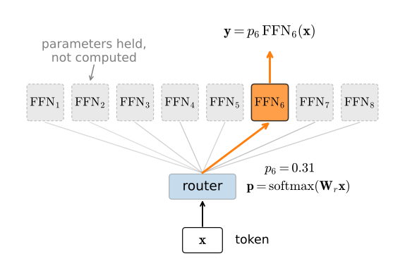
Figure 11.6.1: A mixture-of-experts layer. The router scores all experts for each token; the top-\(k\) (here one) expert runs and its output is weighted by the router probability. Unselected experts hold parameters but perform no computation for this token.

One disclosure about the implementation below: it computes every expert on every token and multiplies by a gate that is zero for the unselected ones. The mathematics of Equation 11.6.1 is exact, but the FLOPs savings of the accounting cell is deliberately not realized — at our scale the dense computation is simpler and plenty fast. Production systems realize the savings with scatter/gather kernels: tokens are physically regrouped per expert, each expert runs one dense batch of its own tokens, and fixed per-expert buffer sizes (the capacity factor, another exercise) keep the shapes static. The teaching implementation preserves the semantics; the accounting carries the economics.

class MoELayer(nn.Module):
    """Mixture-of-experts FFN: a token-choice top-k router over E experts."""
    def __init__(self, num_hiddens, num_experts, num_active):
        super().__init__()
        self.num_experts, self.num_active = num_experts, num_active
        self.router = nn.Linear(num_hiddens, num_experts, bias=False)
        self.experts = nn.ModuleList([d2l.FeedForward(num_hiddens)
                                      for _ in range(num_experts)])
        self.register_buffer('expert_bias', torch.zeros(num_experts))
        self.register_buffer('usage', torch.zeros(num_experts))

    def forward(self, X):
        probs = F.softmax(self.router(X), -1)             # (B, T, E)
        scores = probs + self.expert_bias                 # selection only
        idx = scores.topk(self.num_active, -1).indices    # (B, T, k)
        mask = torch.zeros_like(probs).scatter(-1, idx, 1.0)
        gates = probs * mask                              # weight = p_i
        Y = torch.stack([e(X) for e in self.experts], -1)  # (B, T, d, E)
        out = (Y * gates.unsqueeze(-2)).sum(-1)
        frac = mask.sum((0, 1)) / mask.sum()              # realized load
        self.usage += mask.sum((0, 1)).detach()
        self.aux_loss = self.num_experts * (frac * probs.mean((0, 1))).sum()
        return out

class MoELayer(nnx.Module):
    """Mixture-of-experts FFN: a token-choice top-k router over E experts."""
    def __init__(self, num_hiddens, num_experts, num_active, rngs=None):
        rngs = nnx.Rngs(0) if rngs is None else rngs
        self.num_experts, self.num_active = num_experts, num_active
        self.router = nnx.Linear(num_hiddens, num_experts, use_bias=False,
                                 rngs=rngs)
        self.experts = nnx.List([d2l.FeedForward(num_hiddens, rngs=rngs)
                                 for _ in range(num_experts)])
        self.expert_bias = nnx.Variable(jnp.zeros(num_experts))
        self.usage = nnx.Variable(jnp.zeros(num_experts))
        self.aux_loss = nnx.Variable(jnp.zeros(()))

    def __call__(self, X):
        probs = jax.nn.softmax(self.router(X), -1)        # (B, T, E)
        scores = probs + self.expert_bias[...]            # selection only
        _, idx = jax.lax.top_k(scores, self.num_active)   # (B, T, k)
        mask = jax.nn.one_hot(idx, self.num_experts).sum(-2)
        gates = probs * mask                              # weight = p_i
        Y = jnp.stack([e(X) for e in self.experts], -1)   # (B, T, d, E)
        out = (Y * gates[..., None, :]).sum(-1)
        frac = mask.sum((0, 1)) / mask.sum()              # realized load
        self.usage[...] = self.usage[...] + mask.sum((0, 1))
        self.aux_loss[...] = self.num_experts * (
            frac * probs.mean((0, 1))).sum()
        return out

The dense-gather formulation is also what makes this layer JAX-friendly: token-choice routing hands each expert a data-dependent number of tokens, which XLA’s static shapes cannot express directly. Computing all experts on all tokens keeps every shape fixed; real JAX serving stacks instead fix the shapes with capacity-limited per-expert buffers, exactly the scheme the exercises discuss.

The experts are the d2l.FeedForward of Section 11.1, unchanged. Two buffers ride along for later: expert_bias enters the top-\(k\) selection but never the mixture weights, and usage counts routed tokens — both sit idle until the balancing experiments below. The layer also reports aux_loss, a balance score whose meaning the next section derives; nothing uses it yet. Since MoELayer maps \((n, d)\) to \((n, d)\) like any FFN, it drops into d2l.TransformerBlock through the ffn_factory seam that Section 11.1 built and Section 11.3 already used for attention:

torch.manual_seed(0)
moe = MoELayer(256, num_experts=8, num_active=2)
X = torch.randn(4, 100, 256)
d2l.check_shape(moe(X), X.shape)
blk = d2l.TransformerBlock(256, num_heads=8,
                           ffn_factory=lambda: MoELayer(256, 8, 2))
d2l.check_shape(blk(X), X.shape)
count = lambda m: sum(p.numel() for p in m.parameters())
expert = count(moe.experts[0])
print(f'router {count(moe.router)}, per expert {expert}, total '
      f'{count(moe)}, active '
      f'{count(moe) - (moe.num_experts - moe.num_active) * expert}')
print('usage at initialization: '
      + ' '.join(f'{u:.2f}' for u in moe.usage / moe.usage.sum()))

router 2048, per expert 524544, total 4198400, active 1051136
usage at initialization: 0.13 0.14 0.15 0.10 0.12 0.12 0.11 0.13

moe = MoELayer(256, num_experts=8, num_active=2, rngs=nnx.Rngs(0))
X = jax.random.normal(jax.random.key(0), (4, 100, 256))
d2l.check_shape(moe(X), X.shape)
blk = d2l.TransformerBlock(256, num_heads=8,
                           ffn_factory=lambda rngs: MoELayer(256, 8, 2,
                                                             rngs=rngs))
d2l.check_shape(blk(X), X.shape)
count = lambda m: sum(p.size for p in jax.tree.leaves(
    nnx.state(m, nnx.Param)))
expert = count(moe.experts[0])
print(f'router {count(moe.router)}, per expert {expert}, total '
      f'{count(moe)}, active '
      f'{count(moe) - (moe.num_experts - moe.num_active) * expert}')
print('usage at initialization: '
      + ' '.join(f'{u:.2f}' for u in moe.usage[...] / moe.usage[...].sum()))

router 2048, per expert 524544, total 4198400, active 1051136
usage at initialization: 0.13 0.11 0.13 0.13 0.15 0.12 0.11 0.12

At initialization the picture is as benign as the accounting assumed: a random router spreads random tokens nearly evenly across the eight experts. The interesting question is whether training keeps it that way.

11.6.3 Routing Collapse and Load Balancing

The following notation distinguishes router outputs, selected experts, and measured load.

symbol	meaning
\(E\)	number of stored experts
\(k\)	experts selected per token
\(p_i(\mathbf{x})\)	router probability for expert \(i\) before top-\(k\) selection
\(\mathcal{E}_k(\mathbf{x})\)	selected expert indices for token \(\mathbf{x}\)
\(f_i\)	fraction of routed assignments received by expert \(i\) in a batch
\(\bar p_i\)	batch mean of \(p_i(\mathbf{x})\)
\(b_i\)	non-gradient selection bias used by the auxiliary-loss-free controller

11.6.3.1 Positive Feedback in Routing

Follow the feedback loop. Early in training, random initialization may cause some expert is slightly better than its peers on the tokens it happens to receive. The loss gradient rewards it twice: its parameters improve on those tokens, and the router’s gradient raises its selection probability, because weighting a helpful expert more heavily lowers the loss. More tokens mean more gradient signal, which means a better expert, which attracts more tokens. The experts that lose the early rounds see ever fewer tokens, learn ever more slowly, and their router scores decrease. This feedback can produce routing collapse, in which a few experts receive most assignments and much of the stored capacity is unused. Shazeer et al. (2017) describe this imbalance and introduce load-balancing mechanisms. We next compare two such mechanisms.

11.6.3.2 An Auxiliary Balancing Loss

The classic repair adds a differentiable penalty for imbalance to the training loss. For a batch, let \(f_i\) be the fraction of routed tokens that expert \(i\) received (a count — no gradient flows through it), and let \(\bar{p}_i\) be the router’s mean probability for expert \(i\). The Switch transformer’s loss (Fedus et al. 2022), descended from GShard’s (Lepikhin et al. 2021), is their correlation:

\[ \mathcal{L}_{\mathrm{balance}} = E \sum_{i=1}^{E} f_i\, \bar{p}_i, \tag{11.6.2}\]

added to the language-modeling loss with a small weight \(\alpha\) (0.01 in the Switch paper and below). When routing is uniform, \(f_i = \bar{p}_i = 1/E\) and the loss is exactly \(1\); concentrating tokens on few experts makes \(f\) and \(\bar{p}\) peak together and the correlation grow. Its gradient (through \(\bar{p}\) only) pushes probability away from overloaded experts for every token, whatever the token needs — and that is the cost. The balancing gradient is added to the language-modeling gradient at every step, and the two disagree when some token classes legitimately require a busier expert. Tune \(\alpha\) too high and routing quality degrades; too low and the imbalance persists. This interference is documented rather than hypothetical (Wang et al. 2024), and it motivated the second repair.

11.6.3.3 Balancing Without a Loss

The expert_bias buffer in our layer implements the auxiliary-loss-free scheme of Wang et al. (2024), the one DeepSeek-V3 trains with (DeepSeek-AI et al. 2024). Selection — and only selection — sees a per-expert bias:

\[ \mathcal{E}_k(\mathbf{x}) = \operatorname{argtop}_k \big(p_i(\mathbf{x}) + b_i\big), \qquad b_i \leftarrow b_i + u\, \mathrm{sign}(\bar{f} - f_i), \tag{11.6.3}\]

where \(\bar{f} = 1/E\) is the ideal load and \(u\) is a small update speed. This controller is not part of gradient descent. After each step, the bias of an overloaded expert decreases and that of an underloaded expert increases, making underused experts slightly easier to select. Because \(b_i\) never enters the mixture weight \(p_i\), the loss the model optimizes contains no balancing term at all, so there is no gradient interference to tune away. The controller steers where tokens go; the gradients remain purely about predicting text. One simplification to note: DeepSeek-V3’s router scores experts with per-expert sigmoids and restricts each token’s choices to a few expert groups (which also limits cross-device traffic); our layer keeps the softmax router and changes only the selection bias — the mechanism Wang et al. (2024) isolate.

11.6.3.4 Comparing Balancing Methods at Fixed Compute

Both repairs slot into an ordinary training loop. The trainer below is d2l.train_lm (Section 11.2) plus the two mechanisms, each switched by one argument: aux_weight adds \(\alpha \sum \mathcal{L}_{\mathrm{balance}}\) over the model’s MoE layers, and bias_rate applies the controller of Equation 11.6.3 after each optimizer step. To build the model we take d2l.GPT unchanged and replace each block’s FFN, the same swap-after-construction move Section 11.3 used to install grouped-query attention:

def moe_gpt(vocab_size, num_hiddens, num_blks, num_experts, num_active,
            num_heads=4):
    """A d2l.GPT whose blocks' FFNs are replaced by MoE layers."""
    model = d2l.GPT(vocab_size, num_hiddens=num_hiddens,
                    num_heads=num_heads, num_blks=num_blks)
    for blk in model.blks:
        blk.ffn = MoELayer(num_hiddens, num_experts, num_active)
    return model

def train_moe_lm(model, data, optimizer, num_steps, aux_weight=0.0,
                 bias_rate=0.0):
    """d2l.train_lm plus the two balancing mechanisms."""
    device = d2l.try_gpu()
    model.to(device)
    layers = [blk.ffn for blk in model.blks
              if isinstance(blk.ffn, MoELayer)]
    losses, step = [], 0
    while step < num_steps:
        for X, Y in data.train_dataloader():
            X, Y = X.to(device), Y.to(device)
            logits = model(X)
            ce = F.cross_entropy(logits.reshape(-1, logits.shape[-1]),
                                 Y.reshape(-1))
            loss = ce
            if aux_weight:
                loss = loss + aux_weight * sum(l.aux_loss for l in layers)
            optimizer.zero_grad()
            loss.backward()
            optimizer.step()
            if bias_rate:               # the thermostat: no gradients
                with torch.no_grad():
                    for l in layers:
                        frac = l.usage / l.usage.sum()
                        l.expert_bias += bias_rate * torch.sign(
                            1 / l.num_experts - frac)
                        l.usage.zero_()
            losses.append(ce.item())
            step += 1
            if step >= num_steps:
                return losses

def moe_gpt(vocab_size, num_hiddens, num_blks, num_experts, num_active,
            num_heads=4, rngs=None):
    """A d2l.GPT whose blocks' FFNs are replaced by MoE layers."""
    rngs = nnx.Rngs(0) if rngs is None else rngs
    model = d2l.GPT(vocab_size, num_hiddens=num_hiddens,
                    num_heads=num_heads, num_blks=num_blks, rngs=rngs)
    for blk in model.blks:
        blk.ffn = MoELayer(num_hiddens, num_experts, num_active, rngs=rngs)
    return model

def train_moe_lm(model, data, optimizer, num_steps, aux_weight=0.0,
                 bias_rate=0.0):
    """d2l.train_lm plus the two balancing mechanisms."""
    @nnx.jit
    def step_fn(model, optimizer, X, Y):
        def loss_fn(model):
            logits = model(X)
            ce = optax.softmax_cross_entropy_with_integer_labels(
                logits.reshape(-1, logits.shape[-1]), Y.reshape(-1)).mean()
            aux = sum(blk.ffn.aux_loss[...] for blk in model.blks
                      if isinstance(blk.ffn, MoELayer))
            return ce + aux_weight * aux, ce
        (_, ce), grads = nnx.value_and_grad(loss_fn, has_aux=True)(model)
        optimizer.update(model, grads)
        if bias_rate:                   # the thermostat: no gradients
            for blk in model.blks:
                if isinstance(blk.ffn, MoELayer):
                    l = blk.ffn
                    frac = l.usage[...] / l.usage[...].sum()
                    l.expert_bias[...] = l.expert_bias[...] + bias_rate * (
                        jnp.sign(1 / l.num_experts - frac))
                    l.usage[...] = jnp.zeros_like(l.usage[...])
        return ce
    losses, step = [], 0
    while step < num_steps:
        for X, Y in data.train_dataloader():
            ce = step_fn(model, optimizer, jnp.asarray(X), jnp.asarray(Y))
            losses.append(float(ce))
            step += 1
            if step >= num_steps:
                return losses

Two measurement helpers: validation loss as in Section 11.2, and each layer’s expert-usage distribution over a fixed set of validation batches.

def val_loss(model, data):
    device = d2l.try_gpu()
    model.to(device).eval()
    with torch.no_grad():
        losses = [F.cross_entropy(
            model(X.to(device)).flatten(0, 1), Y.to(device).flatten())
            for X, Y in data.val_dataloader()]
    model.train()
    return sum(l.item() for l in losses) / len(losses)

def usage_fractions(model, data, num_batches=10):
    """Per-layer expert usage over a fixed set of validation batches."""
    device = d2l.try_gpu()
    layers = [blk.ffn for blk in model.blks
              if isinstance(blk.ffn, MoELayer)]
    for l in layers:
        l.usage.zero_()
    model.to(device).eval()
    with torch.no_grad():
        for i, (X, _) in enumerate(data.val_dataloader()):
            if i >= num_batches:
                break
            model(X.to(device))
    model.train()
    return torch.stack([l.usage / l.usage.sum() for l in layers]).cpu()

@nnx.jit
def batch_loss(model, X, Y):
    logits = model(X)
    return optax.softmax_cross_entropy_with_integer_labels(
        logits.reshape(-1, logits.shape[-1]), Y.reshape(-1)).mean()

def val_loss(model, data):
    model.eval()
    losses = [float(batch_loss(model, jnp.asarray(X), jnp.asarray(Y)))
              for X, Y in data.val_dataloader()]
    model.train()
    return sum(losses) / len(losses)

def usage_fractions(model, data, num_batches=10):
    """Per-layer expert usage over a fixed set of validation batches."""
    layers = [blk.ffn for blk in model.blks
              if isinstance(blk.ffn, MoELayer)]
    for l in layers:
        l.usage[...] = jnp.zeros_like(l.usage[...])
    model.eval()
    for i, (X, _) in enumerate(data.val_dataloader()):
        if i >= num_batches:
            break
        model(jnp.asarray(X))
    model.train()
    return jnp.stack([l.usage[...] / l.usage[...].sum() for l in layers])

We train one small model three times from the same initialization on the character-level Time Machine for the same 800 steps: two blocks of width 128, eight experts per block, one active per token (the Switch configuration, where the feedback loop bites hardest). The only difference between the runs is the balancing: none, the auxiliary loss at \(\alpha = 0.01\), or the bias thermostat at \(u = 0.01\).

data = d2l.TimeMachine(batch_size=64, num_steps=128, tokenization='char',
                       num_train=100000, num_val=3000)
results = {}
for name, aux_weight, bias_rate in (('no balancing', 0.0, 0.0),
                                    ('auxiliary loss', 0.01, 0.0),
                                    ('bias', 0.0, 0.01)):
    torch.manual_seed(0)
    model = moe_gpt(len(data.vocab), num_hiddens=128, num_blks=2,
                    num_experts=8, num_active=1)
    losses = train_moe_lm(
        model, data, torch.optim.AdamW(model.parameters(), lr=1e-3,
                                       weight_decay=0.0),
        800, aux_weight, bias_rate)
    results[name] = usage_fractions(model, data)
    print(f'{name:>14}: training loss {sum(losses[-100:])/100:.2f}, '
          f'experts under 2% usage: {int((results[name] < 0.02).sum())} '
          'of 16')

  no balancing: training loss 0.72, experts under 2% usage: 5 of 16
auxiliary loss: training loss 0.66, experts under 2% usage: 0 of 16
          bias: training loss 0.54, experts under 2% usage: 0 of 16

data = d2l.TimeMachine(batch_size=64, num_steps=128, tokenization='char',
                       num_train=100000, num_val=3000)
results = {}
for name, aux_weight, bias_rate in (('no balancing', 0.0, 0.0),
                                    ('auxiliary loss', 0.01, 0.0),
                                    ('bias', 0.0, 0.01)):
    model = moe_gpt(len(data.vocab), num_hiddens=128, num_blks=2,
                    num_experts=8, num_active=1, rngs=nnx.Rngs(0))
    optimizer = nnx.Optimizer(model, optax.adamw(1e-3, weight_decay=0.0),
                              wrt=nnx.Param)
    losses = train_moe_lm(model, data, optimizer, 800, aux_weight,
                          bias_rate)
    results[name] = usage_fractions(model, data)
    print(f'{name:>14}: training loss {sum(losses[-100:])/100:.2f}, '
          f'experts under 2% usage: {int((results[name] < 0.02).sum())} '
          'of 16')

  no balancing: training loss 0.74, experts under 2% usage: 6 of 16
auxiliary loss: training loss 0.53, experts under 2% usage: 0 of 16
          bias: training loss 0.46, experts under 2% usage: 0 of 16

d2l.use_svg_display()
fig, axes = d2l.plt.subplots(1, 3, figsize=(9, 2.8), sharey=True)
x = torch.arange(8)
for ax, (name, u) in zip(axes, results.items()):
    ax.bar(x - 0.2, u[0], 0.4, label='layer 1')
    ax.bar(x + 0.2, u[1], 0.4, label='layer 2')
    ax.axhline(1 / 8, color='gray', ls='--', lw=1)
    ax.set_xlabel('expert')
    ax.set_title(name)
axes[0].set_ylabel('fraction of tokens')
axes[0].legend()

<matplotlib.legend.Legend at 0x7b98db7ec7a0>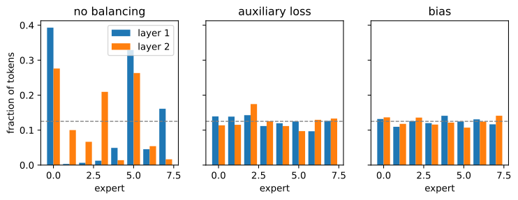

d2l.use_svg_display()
fig, axes = d2l.plt.subplots(1, 3, figsize=(9, 2.8), sharey=True)
x = jnp.arange(8)
for ax, (name, u) in zip(axes, results.items()):
    ax.bar(x - 0.2, u[0], 0.4, label='layer 1')
    ax.bar(x + 0.2, u[1], 0.4, label='layer 2')
    ax.axhline(1 / 8, color='gray', ls='--', lw=1)
    ax.set_xlabel('expert')
    ax.set_title(name)
axes[0].set_ylabel('fraction of tokens')
axes[0].legend()

<matplotlib.legend.Legend at 0x765ee00d91f0>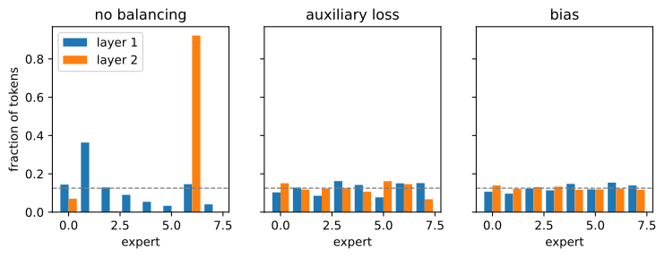

In the displayed seed, the unbalanced run assigns most tokens to a few experts and several experts receive less than 2% of assignments. Both balancing methods produce loads closer to the dashed uniform reference and finish with lower training loss than the unbalanced run. This is one 800-step run per method and framework, so it establishes neither the frequency of routing collapse nor an uncertainty interval for the loss difference. In particular, the overlapping final losses of the two balanced methods do not support a quality ranking. The large-scale motivation for the bias controller comes from the separate experiments of Wang et al. (2024) .

11.6.4 Fine-Grained and Shared Experts

Mixtral’s experts are full-width FFNs, eight complete copies with two active: big specialists, coarsely chosen. The DeepSeek line of models argues for slicing the same budget thinner (Dai et al. 2024). Hold the stored parameters and the active parameters fixed, but make each expert several times narrower and multiply the count and \(k\) accordingly: instead of choosing 2 of 8 experts, choose 8 of 64 quarter-width ones. The active-parameter accounting is identical; what changes is composability. With \(k\) narrow experts a token assembles its FFN from \(\binom{64}{8} \approx 4 \times 10^{9}\) combinations rather than \(\binom{8}{2} = 28\), so specializations can mix and match — one slice for chemistry vocabulary and another for parsing nested clauses, combined on demand rather than fused into one wide monolith.

The second DeepSeek refinement removes a redundancy that fine-grained routing exposes. Every token, whatever its topic, needs some common processing, and with purely routed experts each one must dedicate some of its width to those shared functions. So DeepSeek adds one shared expert that every token passes through unconditionally, alongside its \(k\) routed choices: the common knowledge lives once, in the always-on path, and the routed experts spend their entire width on what actually distinguishes them. Neither refinement changes a line of our layer’s logic — narrower experts change a constructor argument, and the shared expert is one more FFN added outside the router (an exercise builds it). We do not compare granularities in the teaching experiment. Evidence for the refinement comes from the large-scale ablations of Dai et al. (2024) . The following reported configurations show several choices rather than a single converged design:

Table 11.6.1: Routed-expert configurations of deployed MoE language models.

Model	Experts per layer	Active \(k\)	Expert width / \(d\)	Shared expert
Mixtral 8x7B (Jiang et al. 2024)	8	2	3.5	none
DeepSeek-V3 (DeepSeek-AI et al. 2024)	256	8	0.29	1
Qwen3-235B (Yang et al. 2025)	128	8	0.38	none
gpt-oss-120b (OpenAI 2025)	128	4	1.0	none

The three later configurations in the table use more, narrower experts and moderate \(k\). Their shared-expert choices differ: DeepSeek has used one since V2 (DeepSeek-AI 2024), whereas Qwen3 does not. These rows illustrate design variation rather than a universal progression.

11.6.5 A Mixture-of-Experts GPT

We train two models on the same data for the same 600 steps: the dense d2l.GPT of Section 11.2 at width 256 with four blocks, and the same model with every FFN replaced by a mixture of eight experts, one active, balanced by the bias controller. Because the active expert is a full-width FeedForward, the two models have the same per-token computation and nearly the same active parameter count; the MoE stores seven additional inactive experts per block. Since Section 11.2 showed this corpus drives models into memorization within a few hundred steps, we compare the best validation loss over the budget, as Section 11.3 did.

count = lambda m: sum(p.numel() for p in m.parameters())
for name in ('dense', 'MoE'):
    torch.manual_seed(0)
    if name == 'dense':
        model = d2l.GPT(len(data.vocab), num_hiddens=256, num_heads=8,
                        num_blks=4)
    else:
        model = moe_gpt(len(data.vocab), num_hiddens=256, num_blks=4,
                        num_experts=8, num_active=1, num_heads=8)
    optimizer = torch.optim.AdamW(model.parameters(), lr=1e-3,
                                  weight_decay=0.0)
    best = float('inf')
    for chunk in range(6):
        if name == 'dense':
            losses = d2l.train_lm(model, data, optimizer, 100)
        else:
            losses = train_moe_lm(model, data, optimizer, 100,
                                  bias_rate=0.01)
        best = min(best, val_loss(model, data))
    active = count(model)
    if name == 'MoE':
        active -= sum((blk.ffn.num_experts - blk.ffn.num_active)
                      * count(blk.ffn.experts[0]) for blk in model.blks)
    print(f'{name:>5}: {count(model)/1e6:5.2f}M parameters '
          f'({active/1e6:.2f}M active), best validation {best:.2f}, '
          f'final training loss {sum(losses[-50:])/50:.2f}')

dense:  3.16M parameters (3.16M active), best validation 1.51, final training loss 0.21
  MoE: 17.85M parameters (3.16M active), best validation 1.52, final training loss 0.19

count = lambda m: sum(p.size for p in jax.tree.leaves(
    nnx.state(m, nnx.Param)))
for name in ('dense', 'MoE'):
    if name == 'dense':
        model = d2l.GPT(len(data.vocab), num_hiddens=256, num_heads=8,
                        num_blks=4, rngs=nnx.Rngs(0))
    else:
        model = moe_gpt(len(data.vocab), num_hiddens=256, num_blks=4,
                        num_experts=8, num_active=1, num_heads=8,
                        rngs=nnx.Rngs(0))
    optimizer = nnx.Optimizer(model, optax.adamw(1e-3, weight_decay=0.0),
                              wrt=nnx.Param)
    best = float('inf')
    for chunk in range(6):
        if name == 'dense':
            losses = d2l.train_lm(model, data, optimizer, 100)
        else:
            losses = train_moe_lm(model, data, optimizer, 100,
                                  bias_rate=0.01)
        best = min(best, val_loss(model, data))
    active = count(model)
    if name == 'MoE':
        active -= sum((blk.ffn.num_experts - blk.ffn.num_active)
                      * count(blk.ffn.experts[0]) for blk in model.blks)
    print(f'{name:>5}: {count(model)/1e6:5.2f}M parameters '
          f'({active/1e6:.2f}M active), best validation {best:.2f}, '
          f'final training loss {sum(losses[-50:])/50:.2f}')

dense:  3.16M parameters (3.16M active), best validation 1.49, final training loss 0.20
  MoE: 17.85M parameters (3.16M active), best validation 1.49, final training loss 0.17

The mixture holds between five and six times the parameters of the dense baseline at the same active parameter count. In the displayed fixed-seed run, both best validation losses are near 1.5 and the MoE ends with slightly lower training loss. One run cannot establish equivalence, a seed distribution, or the cause of the training-loss difference. It shows that the implementation can route through a larger stored parameter set while keeping the active count matched. Published large-scale studies separately report compute–quality benefits for MoE models (Fedus et al. 2022; Dai et al. 2024).

11.6.6 Summary

A mixture of experts replaces the transformer block’s FFN with \(E\) parallel FFNs and a linear router that sends each token to the top \(k\) of them, weighted by routing probability: parameters scale with \(E\), per-token FLOPs with \(k\). Without balancing, routing can enter a positive-feedback loop in which frequently selected experts receive more updates and become still more likely to be selected. A few experts then process most tokens. The auxiliary balancing loss penalizes the correlation between load and routing probability, but introduces a gradient that can compete with the language-modeling objective; the auxiliary-loss-free bias steers only the top-\(k\) selection through a gradient-free control loop.

In the fixed-seed teaching experiment, both balancing methods move expert loads toward uniformity and finish below the unbalanced training loss. The run does not distinguish the two balancing methods statistically. Published configurations illustrate the capacity–computation separation at larger scale: Mixtral 8x7B stores 46.7B parameters and activates 12.9B per token, while DeepSeek-V3 reports a larger stored-to-active parameter ratio. Some systems use narrower routed experts and an always-active shared expert. Our GPT implementation exposes the same mechanism by replacing the dense FFN.

11.6.7 Exercises

Router gradient. The top-\(k\) selection in Equation 11.6.1 has no gradient, yet the router trains. Consider one token with router logits \(\mathbf{z} = \mathbf{W}_r \mathbf{x}\), so that \(\mathbf{p} = \mathrm{softmax}(\mathbf{z})\), and treat the selected set \(\mathcal{E}_k\) as a constant. Write the layer output as \(\mathbf{y} = \sum_{i \in \mathcal{E}_k} p_i\, \mathrm{FFN}_i(\mathbf{x})\) and let \(s_i = (\partial \mathcal{L} / \partial \mathbf{y})^\top \mathrm{FFN}_i(\mathbf{x})\) be the sensitivity of the loss to expert \(i\)’s output.
1. Derive \(\partial \mathcal{L} / \partial z_j\) for every expert \(j\) in terms of \(\mathbf{p}\) and the \(s_i\). Which logits receive a nonzero gradient, and on which experts’ outputs does the gradient of an unselected logit depend?
2. Mixtral weights the selected experts by renormalized probabilities (Jiang et al. 2024),
  
  \[\tilde{p}_i = \frac{p_i}{\sum_{j \in \mathcal{E}_k} p_j}, \qquad i \in \mathcal{E}_k.\]
  
  Show that for \(k = 1\) the router receives no gradient from the language-modeling loss.
3. Show that for \(k = 2\) with renormalization the output depends on the logits only through the difference \(z_a - z_b\) of the two selected experts \(a\) and \(b\). Which routing decision can the router learn from the loss in this case, and which can it not?
Balancing-loss gradient. The gradient of Equation 11.6.2 flows through \(\bar{p}_i\) only, because \(f_i\) is a count. Consider a batch of \(N\) tokens, and write \(\mathbf{z}(\mathbf{x})\) for the router logits of token \(\mathbf{x}\).
1. Derive \(\partial \mathcal{L}_{\mathrm{balance}} / \partial z_j(\mathbf{x})\). For which experts \(j\) does the gradient step lower the logit of token \(\mathbf{x}\), and for which does it raise it?
2. Show that the gradient vanishes for every token whenever the batch load is uniform, \(f_i = 1/E\), whatever the individual distributions \(\mathbf{p}(\mathbf{x})\) are. Which property of the router does the loss therefore leave unconstrained?
3. Show that the gradient for a token tends to zero as its router distribution approaches a one-hot vector. What does this imply for the ability of the loss to repair a collapse in which the router has become confident?
Serving arithmetic. Qwen3-235B-A22B (Yang et al. 2025) has \(d = 4096\) and 94 layers. Every layer holds 128 SwiGLU experts of width 1536, of which each token activates 8, and no shared expert. Its attention has 64 query heads and 4 key-value heads, each of dimension 128, and its untied embedding and output matrices cover a vocabulary of 151,936 tokens.
1. Use moe_accounting for the experts and the router, and add the attention and embedding parameters as Section 11.6.1 does for Mixtral. Reproduce the 235B stored and 22B active parameters of the model’s name, ignoring normalization weights.
2. How much accelerator memory do the weights need in 16-bit precision? Compare it with the memory of a dense model that has the same per-token computation.
3. Decoding a batch of \(B\) sequences sends one token per sequence through every layer, and its speed is set by the bytes of weights read per step (Section 11.3). Assume that each token selects a uniformly random set of 8 experts, independently of the other tokens. Derive the expected number of distinct experts that a layer reads, and evaluate it for \(B = 1\), 8, and 64. Above which batch size does a step read 90% of the expert weights, and which dense model then reads the same number of bytes per step?
Capacity factor. ● Production MoE systems give each expert a buffer of fixed size for a batch of \(N\) tokens, commonly

\[C = c\, \frac{N k}{E}, \tag{11.6.4}\]

where \(c\) is the capacity factor (Lepikhin et al. 2021; Fedus et al. 2022). Tokens routed to a full expert are dropped: they skip the layer and continue on the residual stream unchanged.
1. Explain why the buffer size must be fixed in advance rather than set by each batch’s routing, when the experts live on different devices.
2. Take \(k = 1\), \(N = 4096\), and a router that sends each token to a uniformly random expert, independently of the other tokens. The load of one expert is then binomial with mean \(N/E\). Use a normal approximation, together with \(\mathbb{E}[\max(Z, 0)] = 1/\sqrt{2\pi}\) for a standard normal \(Z\), to estimate the fraction of tokens dropped at \(c = 1\) for \(E = 8\) and for \(E = 64\). How does the fraction scale with \(E\) and \(N\), and what does \(c = 1.25\) change?
3. What does a large \(c\) cost in memory and in arithmetic when the routing is balanced?
Expert-choice routing. In expert-choice routing (Zhou et al. 2022), the selection runs the other way: each expert takes the \(C = cN/E\) tokens of the batch that assign it the highest router probability, and a token is processed by every expert that took it.
1. Every expert processes exactly \(C\) tokens, so the load is balanced by construction. What is the average number of experts per token, and what are the smallest and largest numbers of experts a single token can receive?
2. Explain why this rule cannot be used as is to train a causal language model that later decodes one token at a time. Consider which positions influence whether a given token is selected.
3. A capacity-limited token-choice layer fills each expert’s buffer in batch order and drops the overflow. Which tokens of the batch can decide whether a given token is processed, and how does the order in which the buffers are filled matter for a causal model?
[code] Feedback-loop ablations. The argument of Section 11.6.3.1 names two reinforcing effects: a frequently selected expert improves on its tokens, and the router gradient raises its selection probability.
1. Stop the gradient at the router logits inside MoELayer, so that \(\mathbf{W}_r\) keeps its initial values while every other parameter trains. Predict whether the no-balancing run of Section 11.6.3.4 still collapses, then rerun it and count the experts under 2% usage. What still changes the routing when \(\mathbf{W}_r\) is fixed?
2. Restore the router gradient and rerun the three runs with num_active=2. Does the unbalanced run still collapse, and as strongly? Use the router gradient of problem 1 to explain how a second active expert changes the signal that the runner-up receives.
[code] Bias controller in isolation. The controller of Equation 11.6.3 can be studied without training. Build MoELayer(256, num_experts=8, num_active=1), draw a fixed batch of shape \((4, 256, 256)\), that is, 1024 standard-normal tokens in four sequences, and add one fixed standard-normal vector \(\boldsymbol{\mu} \in \mathbb{R}^{256}\) to every token, which skews the untrained router toward a few experts. Then repeat 500 times: run the layer on the batch, apply the bias update of train_moe_lm, and reset usage.
1. For \(u \in \{0.001, 0.01, 0.1\}\), plot the largest load \(\max_i f_i\) against the iteration. How does the number of iterations needed to bring it below \(1.5/E\) scale with \(u\), and how does the load behave afterwards?
2. After the last iteration, measure the fraction of tokens whose selected expert differs from the expert with the largest \(p_i(\mathbf{x})\). What determines this fraction, and how does it depend on \(u\)?
3. Replace the sign in Equation 11.6.3 by the raw difference, \(b_i \leftarrow b_i + u' (\bar{f} - f_i)\), with \(u'\) chosen so that the largest first step equals that of \(u = 0.01\). Which behavior from the first sub-problem changes?
[code] Auxiliary-loss weight. ● The comparison of Section 11.6.3.4 fixes \(\alpha = 0.01\) and runs one seed per method.
1. Run the auxiliary-loss configuration with \(\alpha \in \{0, 10^{-3}, 10^{-2}, 10^{-1}, 1\}\), and the bias configuration with \(u = 0.01\), each for seeds 0, 1, and 2. Plot the final training loss and the number of experts under 2% usage against \(\alpha\) with their spread over seeds, and draw the bias runs as a reference.
2. Does the unbalanced run (\(\alpha = 0\)) collapse for every seed? Describe how the training loss depends on \(\alpha\), and explain its behavior at small and at large \(\alpha\) from the two terms of the training objective.
3. At \(\alpha = 0.01\), is the difference in training loss between the auxiliary loss and the bias controller larger than the spread over seeds?
[code] Shared expert. ● Write SharedMoELayer, a subclass of MoELayer that adds the output of one extra d2l.FeedForward, applied to every token with weight one, to the routed mixture (Section 11.6.4). Compare two models in the setup of Section 11.6.3.4, both balanced by the bias controller: MoELayer with \(E = 8\) and \(k = 2\), and SharedMoELayer with 7 routed experts and \(k = 1\). Both store eight experts per layer and activate two per token.
1. Train both for seeds 0, 1, and 2, and compare their best validation losses, evaluated every 100 steps as in Section 11.6.5.
2. Dai et al. (2024) test whether a shared expert holds processing that the routed experts lack: they disable it and activate one more routed expert, which keeps the per-token computation fixed. Repeat this test on a trained SharedMoELayer model. Remove the shared path, set num_active to 2 in every layer, and compare the validation loss with that of the intact model. What does the result say about the division of labor? Why does removing the shared path without the replacement say little about it?
[extended] Expert granularity. ● Section 11.6.4 cites large-scale evidence that narrower, more numerous experts help at a fixed budget, and this section does not test it. In the setup of Section 11.6.3.4, an expert at \(d = 128\) has SwiGLU width 341. Give MoELayer experts of configurable width, and compare \((E, k) \in \{(8, 1), (16, 2), (32, 4), (64, 8)\}\) with expert widths 341, 171, 85, and 43, all balanced by the bias controller. These configurations store and activate the same expert parameters as \((8, 1)\) to within 1%, while the number of expert combinations available to a token grows from 8 to about \(4.4 \times 10^9\).
1. Train each configuration for seeds 0, 1, and 2 and compare the best validation losses. Does finer granularity help at this scale by more than the spread over seeds? Relate the outcome to the ablations of Dai et al. (2024) .
2. The composability argument of Section 11.6.4 assumes that tokens use many different combinations. In one layer of each trained model, record the selected expert set of every token in a fixed set of validation batches, and count the distinct sets that occur. Compare the count with the number of tokens and with the number of available combinations. How much of the added flexibility does the model use?

[code] Sparse dispatch. ● MoELayer evaluates every expert on every token and masks the result, so its arithmetic grows with \(E\) rather than with \(k\). Write a function gathered_moe(layer, X) that returns layer(X) for a MoELayer with num_active=1 while evaluating each expert only on its own tokens: flatten X to shape \((BT, d)\), find the rows routed to each expert with torch.nonzero, apply the expert to those rows, and accumulate the gated outputs with index_add_.
1. Check on random input that gathered_moe(layer, X) agrees with layer(X) up to floating-point error.
2. Time both on an input of shape \((4, 512, 256)\) for \(E \in \{2, 4, 8, 16, 32\}\). From which \(E\) on is the gathered version faster on your hardware? Count the expert FLOPs of each version as a function of \(E\), compare the measured ratio of run times with the ratio of FLOPs, and name the operations of the gathered version that account for the difference.

[code] Capacity-limited dispatch. ● MoELayer evaluates every expert on every token and masks the result, so its arithmetic grows with \(E\) rather than with \(k\). A jitted alternative must keep its shapes static, so each expert receives a buffer of \(C = \lceil cN/E \rceil\) slots for \(N\) tokens. Write a function capacity_moe(layer, X, c) for a MoELayer with num_active=1: flatten X to shape \((N, d)\), compute each token’s slot in its expert’s buffer with jnp.cumsum over the one-hot selection mask, drop the tokens whose slot is at least \(C\), build a dispatch tensor of shape \((N, E, C)\) with jax.nn.one_hot, gather the expert inputs into shape \((E, C, d)\) with jnp.einsum, apply each expert to its buffer, and combine the outputs with the gates.
1. Check on random input that capacity_moe(layer, X, c) with \(c = E\), where nothing is dropped, agrees with layer(X) up to floating-point error.
2. Jit both and time them at \(c = 1.25\) on an input of shape \((4, 512, 256)\) for \(E \in \{2, 4, 8, 16, 32\}\). From which \(E\) on is the dispatch version faster on your hardware? Express the FLOPs of each of its steps in terms of \(N\), \(E\), \(c\), and \(d\), and identify the step that dominates as \(N\) grows at fixed \(E\) and \(c\).