torch.set_float32_matmul_precision('high') # tf32 matmuls on tensor cores17.2 Gaussian Paths: Diffusion and Flow Matching
The previous section ended with a dilemma. At a small noise level a denoiser is accurate near the data, but Langevin chains driven by its score cannot cross the empty valleys between the modes and keep the mode weights they started with; at a large noise level the chains find the right weights but sample a blurred copy of the data. Suppose that one network denoised at every noise level, and that we walked from pure noise down to the data through all of them. How is such a walk defined, which regression trains the network, and how do we take the steps?
Underneath the three routes by which the literature reached the answer (Chapter 17) is one object: a Gaussian path from the data at \(t = 0\) to pure noise at \(t = 1\), the posterior mean of the clean point along it, learned by one regression, and a sampler that integrates the differential equation this posterior mean defines.
Current image, video and audio generators are trained this way. We define the path, derive the regression and its equivalent targets, sample with and without noise, and check the learned models against the exact ones.
17.2.1 One Path from Data to Noise
A walk through all noise levels needs the levels indexed by a time, which this part defines and tests on the mixture.
17.2.1.1 Signal, Noise and the Log-SNR Clock
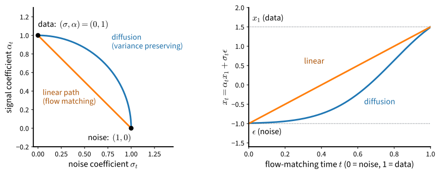
We let the data shrink as the noise grows. A Gaussian path is a pair of functions \(\alpha_t\) and \(\sigma_t\) on \(t \in [0, 1]\) that defines the noisy point
\[ \mathbf{x}_t = \alpha_t\, \mathbf{x}_0 + \sigma_t\, \boldsymbol{\epsilon}, \qquad \boldsymbol{\epsilon} \sim \mathcal{N}(\mathbf{0}, \mathbf{I}), \tag{17.2.1}\]
with \((\alpha_0, \sigma_0) = (1, 0)\) and \((\alpha_1, \sigma_1) = (0, 1)\), or nearly so. The variance-preserving (VP) path keeps \(\alpha_t^2 + \sigma_t^2 = 1\), so data of unit variance keep unit variance; it is the Ornstein–Uhlenbeck process of Section 43.3.3. We write \(\bar\alpha_t := \alpha_t^2\) and use the continuous form of the schedule of Ho et al. (2020), \(\log \bar\alpha_t = -\big(\beta_{\min} t + (\beta_{\max} - \beta_{\min})\, t^2/2\big)\) with \(\beta_{\min} = 0.1\) and \(\beta_{\max} = 20\). The linear path of flow matching and rectified flow (Lipman et al. 2023; Liu et al. 2023; Albergo et al. 2023) draws a straight line from the data to the noise,
\[ \alpha_t = 1 - t, \qquad \sigma_t = t. \tag{17.2.2}\]
What a denoiser can infer from \(\mathbf{x}_t\) depends only on the ratio of signal to noise, measured on a log scale as the log-SNR \(\lambda_t = \log(\alpha_t^2 / \sigma_t^2)\). It falls monotonically from \(+\infty\) at the data to \(-\infty\) at the noise, a clock that all paths share: at times of equal \(\lambda\), two paths hold the same noisy point up to a scale factor (7). The VP path reaches \(\bar\alpha_1 = e^{-10.05} \approx 4 \cdot 10^{-5}\) at \(t = 1\), close enough to pure noise (Figure 17.2.1).
ImportantOne clock
Data sit at \(t = 0\) and noise at \(t = 1\) throughout the book (Section 43.6), and every sampler runs from \(t = 1\) down to \(0\). Flow-matching papers reverse time (Figure 43.6.1): substitute \(1 - t\) for their \(t\), read their noise \(\mathbf{x}_0\) as our \(\boldsymbol\epsilon\) and their data \(\mathbf{x}_1\) as our \(\mathbf{x}_0\), and flip the sign of every velocity.
GaussianPath holds the two functions \(\alpha_t\) and \(\sigma_t\), the log-SNR and a draw of \(\mathbf{x}_t\); vp, linear and cosine build the paths of this section.
class GaussianPath:
    """x_t = alpha(t) x0 + sigma(t) eps, data at t = 0 and noise at t = 1."""
    def __init__(self, alpha, sigma):
        self.alpha, self.sigma = alpha, sigma

    @staticmethod
    def vp(beta_min=0.1, beta_max=20.0):
        """Variance preserving, Ho et al.'s linear beta in continuous time."""
        log_abar = lambda t: -(beta_min * t + (beta_max - beta_min) * t**2 / 2)
        return GaussianPath(lambda t: torch.exp(log_abar(t) / 2),
                            lambda t: torch.sqrt(-torch.expm1(log_abar(t))))

    @staticmethod
    def linear():
        """The straight line of flow matching and rectified flow."""
        return GaussianPath(lambda t: 1 - t, lambda t: t)

    @staticmethod
    def cosine(s=0.008):
        """Variance preserving, Nichol and Dhariwal's cosine schedule."""
        c = lambda t: torch.cos(math.pi / 2 * (t + s) / (1 + s))
        g = lambda t: c(t) / c(torch.zeros_like(t))   # exactly 1 at t = 0
        # and exactly 0 at t = 1 (cos(pi/2) is not), keeping the slope
        f = lambda t: torch.where(t < 1, g(t), g(t) - g(t).detach())
        return GaussianPath(f, lambda t: torch.sqrt(1 - f(t) ** 2))

    def log_snr(self, t):
        """lambda_t = log(alpha_t^2 / sigma_t^2), falling from +inf at 0."""
        return 2 * (torch.log(self.alpha(t)) - torch.log(self.sigma(t)))

    def sample(self, x0, t, eps):
        """x_t for per-example times t of shape (n,)."""
        t = t.reshape(-1, *[1] * (x0.dim() - 1))
        return self.alpha(t) * x0 + self.sigma(t) * eps
class GaussianPath:
"""x_t = alpha(t) x0 + sigma(t) eps, data at t = 0 and noise at t = 1."""
def __init__(self, alpha, sigma):
self.alpha, self.sigma = alpha, sigma
@staticmethod
def vp(beta_min=0.1, beta_max=20.0):
"""Variance preserving, Ho et al.'s linear beta in continuous time."""
log_abar = lambda t: -(beta_min * t + (beta_max - beta_min) * t**2 / 2)
return GaussianPath(lambda t: jnp.exp(log_abar(t) / 2),
lambda t: jnp.sqrt(-jnp.expm1(log_abar(t))))
@staticmethod
def linear():
"""The straight line of flow matching and rectified flow."""
return GaussianPath(lambda t: 1 - t, lambda t: t)
@staticmethod
def cosine(s=0.008):
"""Variance preserving, Nichol and Dhariwal's cosine schedule."""
c = lambda t: jnp.cos(math.pi / 2 * (t + s) / (1 + s))
g = lambda t: c(t) / c(jnp.zeros_like(t)) # exactly 1 at t = 0
# and exactly 0 at t = 1 (cos(pi/2) is not), keeping the slope
f = lambda t: jnp.where(t < 1, g(t),
g(t) - jax.lax.stop_gradient(g(t)))
return GaussianPath(f, lambda t: jnp.sqrt(1 - f(t) ** 2))
def log_snr(self, t):
"""lambda_t = log(alpha_t^2 / sigma_t^2), falling from +inf at 0."""
return 2 * (jnp.log(self.alpha(t)) - jnp.log(self.sigma(t)))
def sample(self, x0, t, eps):
"""x_t for per-example times t of shape (n,)."""
t = t.reshape(-1, *[1] * (x0.ndim - 1))
return self.alpha(t) * x0 + self.sigma(t) * epsWe print both coefficients and the log-SNR at three times.
vp, linear = GaussianPath.vp(), GaussianPath.linear()
t = torch.tensor([0.1, 0.5, 0.9])
r2 = lambda v: [round(u, 2) for u in v.tolist()]
for name, path in (('vp', vp), ('linear', linear)):
    print(f'{name:>6}: alpha {r2(path.alpha(t))} sigma {r2(path.sigma(t))} '
          f'log-SNR {r2(path.log_snr(t))}')
vp: alpha [0.95, 0.28, 0.02] sigma [0.32, 0.96, 1.0] log-SNR [2.16, -2.46, -8.15]
linear: alpha [0.9, 0.5, 0.1] sigma [0.1, 0.5, 0.9] log-SNR [4.39, 0.0, -4.39]vp, linear = GaussianPath.vp(), GaussianPath.linear()
t = jnp.array([0.1, 0.5, 0.9])
r2 = lambda v: [round(float(u), 2) for u in v]
for name, path in (('vp', vp), ('linear', linear)):
print(f'{name:>6}: alpha {r2(path.alpha(t))} sigma {r2(path.sigma(t))} '
f'log-SNR {r2(path.log_snr(t))}') vp: alpha [0.95, 0.28, 0.02] sigma [0.32, 0.96, 1.0] log-SNR [2.16, -2.46, -8.15]
linear: alpha [0.9, 0.5, 0.1] sigma [0.1, 0.5, 0.9] log-SNR [4.39, 0.0, -4.39]Halfway along in time the VP path is already mostly noise, with \(\bar\alpha = 0.079\) and \(\lambda \approx -2.5\) against \(\lambda = 0\) on the linear path, and at \(t = 0.9\) it keeps less than two percent of the signal against ten percent.
17.2.1.2 The Chain View
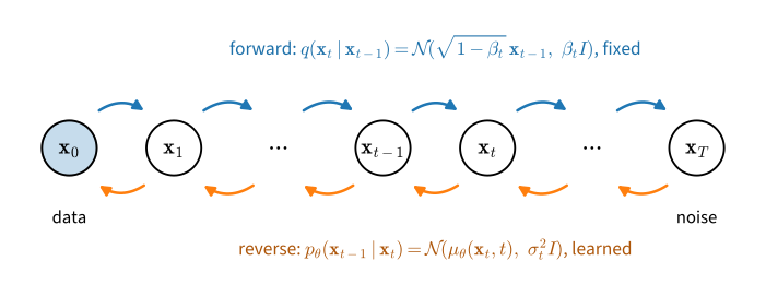
The forward process of Ho et al. (2020) is a Markov chain of \(T\) small steps, each shrinking the current point and adding a little noise,
\[ \mathbf{x}_k = \sqrt{1 - \beta_k}\, \mathbf{x}_{k-1} + \sqrt{\beta_k}\, \boldsymbol{\epsilon}_k, \qquad k = 1, \ldots, T, \tag{17.2.3}\]
with independent standard Gaussians \(\boldsymbol\epsilon_k\) and a variance schedule \(\beta_k \in (0, 1)\). Each step preserves unit variance, and because the noises are independent Gaussians, consecutive steps compose into one: the marginal of every step is a single draw,
\[ \mathbf{x}_k = \sqrt{\bar\alpha_k}\, \mathbf{x}_0 + \sqrt{1 - \bar\alpha_k}\, \boldsymbol{\epsilon}, \qquad \bar\alpha_k = \prod_{j=1}^{k} (1 - \beta_j), \tag{17.2.4}\]
which Section 43.5.3.2 proves by induction. With \(\beta_k = 1 - \bar\alpha_{t_k} / \bar\alpha_{t_{k-1}}\) the DDPM step is the exact transition of the VP path from \(t_{k-1}\) to \(t_k\), so the chain is the VP path read on the grid \(t_k = k/T\). Training never simulates the chain, because any \(\mathbf{x}_k\) is one Gaussian draw away from \(\mathbf{x}_0\). Figure 17.2.2 shows the forward chain and the reverse chain that generation runs.
grid evaluates the path at even times from noise down to data, the grid every sampler steps along; a start time below 1 begins partway along the path.
@d2l.add_to_class(GaussianPath)
def grid(self, steps, t_start=1.0, t_end=0.0):
    """Lists of alpha and sigma at steps + 1 even times, t_start to t_end."""
    t = torch.linspace(t_start, t_end, steps + 1, dtype=torch.float64)
return self.alpha(t).tolist(), self.sigma(t).tolist()@d2l.add_to_class(GaussianPath)
def grid(self, steps, t_start=1.0, t_end=0.0):
"""Arrays of alpha and sigma at steps + 1 even times, t_start to t_end."""
with jax.ensure_compile_time_eval(): # constants, even under jit
t = jnp.linspace(t_start, t_end, steps + 1)
return self.alpha(t), self.sigma(t)Which schedule does our VP path define on a grid of \(T = 1000\) steps? The grid lists the times from the noise end, so its first entries belong to the last step of the chain.
a, _ = vp.grid(1000)
print(f'beta_1 = {1 - (a[-2] / a[-1]) ** 2:.1e}, '
      f'beta_T = {1 - (a[0] / a[1]) ** 2:.4f}, alpha_bar_T = {a[0] ** 2:.1e}')
beta_1 = 1.1e-04, beta_T = 0.0198, alpha_bar_T = 4.3e-05a, _ = vp.grid(1000)
print(f'beta_1 = {1 - (a[-2] / a[-1]) ** 2:.1e}, '
f'beta_T = {1 - (a[0] / a[1]) ** 2:.4f}, alpha_bar_T = {a[0] ** 2:.1e}')beta_1 = 1.1e-04, beta_T = 0.0198, alpha_bar_T = 4.3e-05The steps grow from about \(10^{-4}\) at the data to \(0.02\) at the noise, the linear schedule of Ho et al. (2020), and after a thousand steps only a factor \(\sqrt{\bar\alpha_T} \approx 0.007\) of the data survives.
17.2.1.3 Annealing through Noise Levels
Does a walk through many noise levels do what one level could not? Because the scores of the smoothed mixture are known exactly, we can test this before training any network. We run the Langevin sampler Equation 17.1.11 down a ladder of noise levels: ten levels \(\tilde\sigma_i\) spaced evenly in log scale from \(3\) down to \(0.05\), each with \(100\) steps of size \(h_i = 0.1\, \tilde\sigma_i^2\) on the exact score of \(p_{\tilde\sigma_i}\), starting where the previous level stopped. The control spends the same \(1{,}000\) steps at the finest level, with the step size \(h = 0.05\) of the previous section. Both start from the same \(2{,}000\) points drawn from \(\mathcal{N}(\mathbf{0}, 9\mathbf{I})\).
torch.manual_seed(0)
device = d2l.try_gpu()
mix = d2l.GaussianMixture.three_modes(device)
x_init = 3 * torch.randn(2000, 2, device=device)
x = x_init
for s in torch.logspace(math.log10(3), math.log10(0.05), 10).tolist():
    x = d2l.langevin(lambda z: mix.score(z, 1.0, s), x, 0.1 * s ** 2, 100)
control = d2l.langevin(lambda z: mix.score(z, 1.0, 0.05), x_init, 0.05, 1000)
print('finest level only:', mix.summary(control))
print('ten levels:       ', mix.summary(x))
d2l.scatter_panels([control, x], ['finest level only', 'ten levels'],
                   data=mix.sample(2000));
finest level only: {'weights': [0.339, 0.331, 0.33], 'stray': 0.0145, 'spread': 0.493}
ten levels: {'weights': [0.496, 0.297, 0.208], 'stray': 0.015, 'spread': 0.516}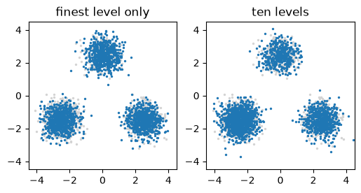
key = jax.random.key(0)
mix = d2l.GaussianMixture.three_modes()
key, k_init, k_ctrl, k_data = jax.random.split(key, 4)
x_init = 3 * jax.random.normal(k_init, (2000, 2))
x = x_init
for s in jnp.logspace(math.log10(3), math.log10(0.05), 10).tolist():
    key, k = jax.random.split(key)
    x = d2l.langevin(lambda z: mix.score(z, 1.0, s), x, 0.1 * s ** 2, 100, k)
control = d2l.langevin(lambda z: mix.score(z, 1.0, 0.05), x_init, 0.05, 1000,
                       k_ctrl)
print('finest level only:', mix.summary(control))
print('ten levels:       ', mix.summary(x))
d2l.scatter_panels([control, x], ['finest level only', 'ten levels'],
                   data=mix.sample(k_data, 2000));
finest level only: {'weights': [0.312, 0.346, 0.342], 'stray': 0.017, 'spread': 0.511}
ten levels: {'weights': [0.478, 0.305, 0.218], 'stray': 0.0165, 'spread': 0.508}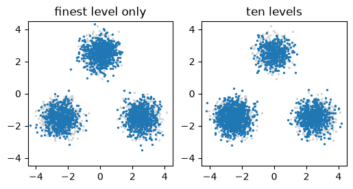
The ladder lands within about \(0.03\) of the weights \(0.5/0.3/0.2\), with one to two percent of the points straying between the modes. The control has the right spread around each mode but keeps the weights of its starting points, about a third each. The proportions are decided at the coarse levels, where the smoothed density has no valleys; the fine levels only sharpen each mode. A diffusion model divides the work the same way along its path.
This annealed Langevin dynamics sampled the first generator of this kind (Song and Ermon 2019), one network that takes the noise level as input, trained by denoising score matching at every level of the ladder with weights \(\tilde\sigma_i^2\) (Section 43.5.3, 3). Its levels, step sizes and step counts were designed by hand (8). The path replaces the ladder by a continuum of levels, and a sampler that the path determines replaces the hand-tuned Langevin steps.
17.2.2 One Regression
One network is to serve every point of the path. What should it learn at a noisy point, which regression teaches it, and how do the targets of the literature relate?
17.2.2.1 Conditional Targets and Marginal Fields
The object to learn is again the posterior mean of the clean point, \(\hat{\mathbf{x}}_0 = \mathbb{E}[\mathbf{x}_0 \mid \mathbf{x}_t]\), which gave the score by Tweedie’s formula Equation 17.1.5 and also tells a noisy point which way to move. It depends on the whole data distribution and is unknown, but its conditional version is trivial: given \(\mathbf{x}_0\), the best guess of \(\mathbf{x}_0\) is \(\mathbf{x}_0\) itself.
The same holds for motion along the path. A single noisy point moves along \(\mathbf{x}_t = \alpha_t \mathbf{x}_0 + \sigma_t \boldsymbol\epsilon\) with the conditional velocity \(\dot{\mathbf{x}}_t = \dot\alpha_t \mathbf{x}_0 + \dot\sigma_t \boldsymbol\epsilon\), which on the linear path is \(\boldsymbol\epsilon - \mathbf{x}_0\). The whole cloud of noisy points moves at \(\mathbf{x}\) with the average velocity of the points that pass there,
\[ \mathbf{u}_t(\mathbf{x}) = \mathbb{E}\big[\dot\alpha_t\, \mathbf{x}_0 + \dot\sigma_t\, \boldsymbol\epsilon \,\big|\, \mathbf{x}_t = \mathbf{x}\big], \tag{17.2.5}\]
the marginal velocity. Where only one clean point can have produced \(\mathbf{x}\), it is that point’s velocity; where several can, it is their average, weighted by how likely each is.
A field defined as a conditional expectation is learned by regressing on the quantity inside it, because least squares recovers the conditional mean; this is how denoising score matching recovered the score. For the velocity it gives the conditional flow matching loss, which differs from the regression onto the unknown marginal field only by a constant \(C\) that does not depend on the network:
\[ \mathbb{E}_{t,\, \mathbf{x}_0,\, \boldsymbol\epsilon}\, \big\| \mathbf{u}_{\boldsymbol\theta}(\mathbf{x}_t, t) - (\dot\alpha_t \mathbf{x}_0 + \dot\sigma_t \boldsymbol\epsilon) \big\|^2 = \mathbb{E}_{t,\, \mathbf{x}_t}\, \big\| \mathbf{u}_{\boldsymbol\theta}(\mathbf{x}_t, t) - \mathbf{u}_t(\mathbf{x}_t) \big\|^2 + C. \tag{17.2.6}\]
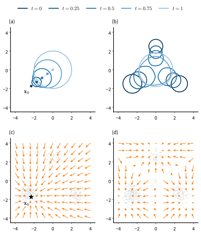
The two sides have the same minimizer, so a network trained on the per-example velocity learns the marginal one (Section 43.6.1). Figure 17.2.3 shows both views.
target gives the per-example regression target of a kind on any path. For 'velocity' it is the conditional velocity, with \(\dot\alpha_t\) and \(\dot\sigma_t\) from forward-mode differentiation (rates); x0_eps turns a prediction of any kind back into the pair \((\hat{\mathbf{x}}_0, \hat{\boldsymbol\epsilon})\).
@d2l.add_to_class(GaussianPath)
def rates(self, t):
    """The time derivatives (alpha'(t), sigma'(t)), by forward-mode AD."""
    ones = torch.ones_like(t)
    return (torch.func.jvp(self.alpha, (t,), (ones,))[1],
            torch.func.jvp(self.sigma, (t,), (ones,))[1])

@d2l.add_to_class(GaussianPath)
def target(self, kind, x0, eps, t):
    """The regression target of a kind: eps, x0, v, score or velocity."""
    t = t.reshape(-1, *[1] * (x0.dim() - 1))
    a, s = self.alpha(t), self.sigma(t)
    if kind == 'eps': return eps
    if kind == 'x0': return x0
    if kind == 'v': return a * eps - s * x0
    if kind == 'score': return -eps / s
    if kind != 'velocity': raise ValueError(f'unknown kind {kind!r}')
    da, ds = self.rates(t)                      # velocity = d x_t / dt
    return da * x0 + ds * eps

@d2l.add_to_class(GaussianPath)
def x0_eps(self, kind, out, x, t):
    """The (x0, eps) that a prediction `out` of a kind implies at (x, t)."""
    t = t.reshape(-1, *[1] * (x.dim() - 1))
    a, s = self.alpha(t), self.sigma(t)
    if kind == 'eps': return (x - s * out) / a, out
    if kind == 'x0': return out, (x - a * out) / s
    if kind == 'v': return ((a * x - s * out) / (a**2 + s**2),
                            (s * x + a * out) / (a**2 + s**2))
    if kind == 'score': return (x + s ** 2 * out) / a, -s * out
    if kind != 'velocity': raise ValueError(f'unknown kind {kind!r}')
    da, ds = self.rates(t)
    det = a * ds - s * da
return (ds * x - s * out) / det, (a * out - da * x) / det@d2l.add_to_class(GaussianPath)
def rates(self, t):
"""The time derivatives (alpha'(t), sigma'(t)), by forward-mode AD."""
ones = jnp.ones_like(t)
return (jax.jvp(self.alpha, (t,), (ones,))[1],
jax.jvp(self.sigma, (t,), (ones,))[1])
@d2l.add_to_class(GaussianPath)
def target(self, kind, x0, eps, t):
"""The regression target of a kind: eps, x0, v, score or velocity."""
t = t.reshape(-1, *[1] * (x0.ndim - 1))
a, s = self.alpha(t), self.sigma(t)
if kind == 'eps': return eps
if kind == 'x0': return x0
if kind == 'v': return a * eps - s * x0
if kind == 'score': return -eps / s
if kind != 'velocity': raise ValueError(f'unknown kind {kind!r}')
da, ds = self.rates(t) # velocity = d x_t / dt
return da * x0 + ds * eps
@d2l.add_to_class(GaussianPath)
def x0_eps(self, kind, out, x, t):
"""The (x0, eps) that a prediction `out` of a kind implies at (x, t)."""
t = t.reshape(-1, *[1] * (x.ndim - 1))
a, s = self.alpha(t), self.sigma(t)
if kind == 'eps': return (x - s * out) / a, out
if kind == 'x0': return out, (x - a * out) / s
if kind == 'v': return ((a * x - s * out) / (a**2 + s**2),
(s * x + a * out) / (a**2 + s**2))
if kind == 'score': return (x + s ** 2 * out) / a, -s * out
if kind != 'velocity': raise ValueError(f'unknown kind {kind!r}')
da, ds = self.rates(t)
det = a * ds - s * da
return (ds * x - s * out) / det, (a * out - da * x) / detThe method fits in one cell. Each step draws \(512\) fresh points from the mixture and a time and a noise for each, and regresses TimeMLP onto the conditional velocity of the linear path, for \(40{,}000\) Adam steps with a cosine-decayed learning rate; train_regression also returns a moving average of the weights with a half-life of \(700\) steps.
def regression_loss(path, kind):
    """Squared error of net(x_t, t) against the target of a kind, t ~ U(0, 1)."""
    def loss_fn(net, x0):
        t = torch.rand(len(x0), device=x0.device)
        eps = torch.randn_like(x0)
        error = net(path.sample(x0, t, eps), t) - path.target(kind, x0, eps, t)
        return (error ** 2).flatten(1).sum(1).mean()  # ||error||^2 per example
    return loss_fn

torch.manual_seed(1)
num_steps = 40_000
net_v, ema_v, losses_v = d2l.train_regression(
    d2l.TimeMLP(256, 3).to(device), regression_loss(linear, 'velocity'),
    lambda: mix.sample(512), num_steps, cosine=True, ema_half_life=700)
d2l.plot(torch.arange(100) * num_steps // 100,
         losses_v.reshape(100, -1).mean(1).cpu(), 'step', 'loss')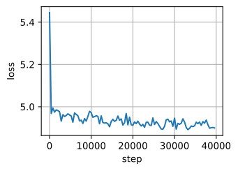
def regression_loss(path, kind):
    """Squared error of net(x_t, t) against the target of a kind, t ~ U(0, 1)."""
    def loss_fn(net, x0, key):
        k_t, k_eps = jax.random.split(key)
        t = jax.random.uniform(k_t, (len(x0),))
        eps = jax.random.normal(k_eps, x0.shape)
        error = net(path.sample(x0, t, eps), t) - path.target(kind, x0, eps, t)
        return (error ** 2).reshape(len(x0), -1).sum(1).mean()  # per example
    return loss_fn

num_steps = 40_000
net_v, ema_v, losses_v = d2l.train_regression(
    d2l.TimeMLP(256, 3, rngs=nnx.Rngs(1)), regression_loss(linear, 'velocity'),
    lambda k: mix.sample(k, 512), num_steps, jax.random.key(1), cosine=True,
    ema_half_life=700)
d2l.plot(jnp.arange(100) * num_steps // 100,
         losses_v.reshape(100, -1).mean(1), 'step', 'loss')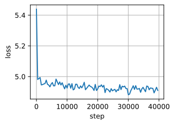
Each point of the curve averages \(400\) steps. The loss falls within a few thousand steps and levels off near \(5\), far above zero; we will see that no network can do much better.
17.2.2.2 Four Targets, One Oracle
The network above predicts a velocity; DDPM’s predicts the noise, and others predict the clean point. At a fixed \(\mathbf{x}_t\) these are not different quantities. Taking the posterior mean of Equation 17.2.1 gives \(\mathbf{x}_t = \alpha_t \hat{\mathbf{x}}_0 + \sigma_t \hat{\boldsymbol\epsilon}\), so \(\hat{\boldsymbol\epsilon} = \mathbb{E}[\boldsymbol\epsilon \mid \mathbf{x}_t]\) and \(\hat{\mathbf{x}}_0\) determine each other, and Tweedie’s formula for the kernel \(\mathcal{N}(\alpha_t \mathbf{x}_0, \sigma_t^2 \mathbf{I})\) gives the score, as in Equation 17.1.6:
\[ \nabla \log p_t(\mathbf{x}_t) = \frac{\alpha_t \hat{\mathbf{x}}_0 - \mathbf{x}_t}{\sigma_t^2} = -\frac{\hat{\boldsymbol\epsilon}}{\sigma_t}. \tag{17.2.7}\]
The marginal velocity Equation 17.2.5 is \(\dot\alpha_t \hat{\mathbf{x}}_0 + \dot\sigma_t \hat{\boldsymbol\epsilon}\), and eliminating \(\hat{\mathbf{x}}_0\) between it and the score gives the score–velocity identity
\[ \mathbf{u}_t(\mathbf{x}) = \frac{\dot\alpha_t}{\alpha_t}\, \mathbf{x} - \Big(\sigma_t \dot\sigma_t - \sigma_t^2 \frac{\dot\alpha_t}{\alpha_t}\Big) \nabla \log p_t(\mathbf{x}), \tag{17.2.8}\]
with multiples fixed by the path. On the linear path it reads
\[ \mathbf{u}_t(\mathbf{x}) = \hat{\boldsymbol\epsilon} - \hat{\mathbf{x}}_0 = -\frac{\mathbf{x} + t\, \nabla \log p_t(\mathbf{x})}{1 - t}. \tag{17.2.9}\]
A fifth target, \(\mathbf{v} = \alpha_t \boldsymbol\epsilon - \sigma_t \mathbf{x}_0\), was introduced by Salimans and Ho (2022) as \(\mathbf{v}\)-prediction; on the cosine path \(\alpha_t = \cos\frac{\pi t}{2}\), \(\sigma_t = \sin\frac{\pi t}{2}\) it equals \(2/\pi\) times the velocity. All of these are affine functions of one posterior mean, the oracle that a perfect network would learn, so a network trained on any of them defines all of them (Table 43.6.1 collects the conversions). The named models of the literature are choices of path and target (Table 17.2.1).
DDPM’s training loss, which Ho et al. (2020) called the simple loss, is
\[ L_{\textrm{simple}}(\boldsymbol\theta) = \mathbb{E}_{t,\, \mathbf{x}_0,\, \boldsymbol\epsilon}\, \big\| \boldsymbol\epsilon - \boldsymbol\epsilon_{\boldsymbol\theta}(\alpha_t \mathbf{x}_0 + \sigma_t \boldsymbol\epsilon,\, t) \big\|^2 . \tag{17.2.10}\]
Since the conditional score of the kernel is \(-\boldsymbol\epsilon/\sigma_t\), the simple loss is denoising score matching Equation 17.1.3 at every level, weighted by \(\sigma_t^2\) (Section 43.5.3.2). Ho et al. derived it from a variational bound on the log-likelihood; with one particular weighting over \(t\) the regression is such a bound (Section 17.5).
target and x0_eps above implement these conversions. make_pred wraps a trained network as the pair \((\hat{\mathbf{x}}_0, \hat{\boldsymbol\epsilon})\) at any \((\alpha, \sigma)\), by querying it at the time of its own path with the same log-SNR, which time_at finds by bisection. An \(\boldsymbol\epsilon\)-predictor has no \(\hat{\mathbf{x}}_0 = (\mathbf{x} - \sigma\hat{\boldsymbol\epsilon})/\alpha\) at pure noise, \(\alpha = 0\), so samplers that start there on the linear and cosine paths need another kind; an \(\boldsymbol\epsilon\)-model samples on the VP path, whose \(\alpha\) stays positive.
@d2l.add_to_class(GaussianPath)
def time_at(self, log_snr):
    """The time with a given log-SNR, by bisection (lambda_t falls in t)."""
    lo, hi = torch.zeros_like(log_snr), torch.ones_like(log_snr)
    for _ in range(50):
        mid = (lo + hi) / 2
        later = self.log_snr(mid) > log_snr      # the answer lies after mid
        lo, hi = torch.where(later, mid, lo), torch.where(later, hi, mid)
    return (lo + hi) / 2

def make_pred(net, path, kind):
    """pred(x, alpha, sigma) -> (x0, eps) from net(x, t) of a kind on path."""
    def pred(x, alpha, sigma):
        log_snr = 2 * math.log(alpha / sigma) if alpha > 0 else -math.inf
        t = path.time_at(torch.tensor(log_snr, dtype=torch.float64))
        x = x * (path.sigma(t).item() / sigma)  # the same point on our path
        t = torch.full((len(x),), t.item(), device=x.device)
        return path.x0_eps(kind, net(x, t), x, t)
return pred@d2l.add_to_class(GaussianPath)
def time_at(self, log_snr):
"""The time with a given log-SNR, by bisection (lambda_t falls in t)."""
def halve(_, interval):
lo, hi = interval
mid = (lo + hi) / 2
later = self.log_snr(mid) > log_snr # the answer lies after mid
return jnp.where(later, mid, lo), jnp.where(later, hi, mid)
lo, hi = jax.lax.fori_loop(0, 50, halve, (jnp.zeros_like(log_snr),
jnp.ones_like(log_snr)))
return (lo + hi) / 2
def make_pred(net, path, kind):
"""pred(x, alpha, sigma) -> (x0, eps) from net(x, t) of a kind on path."""
def pred(x, alpha, sigma):
log_snr = jnp.where(alpha > 0, 2 * jnp.log(alpha / sigma), -jnp.inf)
t = path.time_at(jnp.asarray(log_snr, jnp.float32))
x = x * (path.sigma(t) / sigma) # the same point on our path
t = jnp.full((len(x),), t)
return path.x0_eps(kind, net(x, t), x, t)
return predThe second model makes DDPM’s choice, the noise target on the VP path, and changes nothing else.
torch.manual_seed(2)
net_eps, ema_eps, losses_eps = d2l.train_regression(
    d2l.TimeMLP(256, 3).to(device), regression_loss(vp, 'eps'),
    lambda: mix.sample(512), num_steps, cosine=True, ema_half_life=700)
net_eps, ema_eps, losses_eps = d2l.train_regression(
d2l.TimeMLP(256, 3, rngs=nnx.Rngs(2)), regression_loss(vp, 'eps'),
lambda k: mix.sample(k, 512), num_steps, jax.random.key(2), cosine=True,
ema_half_life=700)The two networks differ in path and target, but by the dictionary they should hold the same posterior mean, which the last part of the section checks.
17.2.2.3 The Loss Floor
The velocity model’s loss levelled off near \(5\) for the reason of Section 17.1: a target contains the noise of its own example, so even the oracle keeps the conditional variance of the target given \(\mathbf{x}_t\), now averaged over the path. For the mixture this floor is exact. The function oracle takes \(\hat{\mathbf{x}}_0\) from GaussianMixture.posterior_mean and \(\hat{\boldsymbol\epsilon}\) from \(\mathbf{x}_t = \alpha_t \hat{\mathbf{x}}_0 + \sigma_t \hat{\boldsymbol\epsilon}\); every target is the same affine function of them, and any sampler can use oracle in place of a network.
def oracle(x, alpha, sigma):
    """The exact posterior means (x0_hat, eps_hat) of the mixture at x."""
    x0_hat = mix.posterior_mean(x, alpha, sigma)
    a, s = (torch.as_tensor(v, device=x.device).reshape(-1, 1)
            for v in (alpha, sigma))
    return x0_hat, (x - a * x0_hat) / s

def loss_floor(path, kind, x0, eps, t):
    """E||target - E[target | x_t]||^2 over the draws (x0, eps, t)."""
    x = path.sample(x0, t, eps)
    best = path.target(kind, *oracle(x, path.alpha(t), path.sigma(t)), t)
    return ((path.target(kind, x0, eps, t) - best) ** 2).sum(1).mean().item()

n = 1_000_000
x0, eps = mix.sample(n), torch.randn(n, 2, device=device)
times = [torch.full((n,), t, device=device) for t in (0.1, 0.5, 0.9)]
times.append(torch.rand(n, device=device))             # t ~ U(0, 1)
print('target, path      t=0.1  t=0.5  t=0.9  t~U(0,1)  trained')
for name, path, kind, losses in (('noise, vp', vp, 'eps', losses_eps),
        ('velocity, linear', linear, 'velocity', losses_v)):
    floors = [loss_floor(path, kind, x0, eps, t) for t in times]
    print(f'{name:16}' + ''.join(f'{f:7.3f}' for f in floors[:3])
          + f'{floors[3]:10.3f}{losses[-1000:].mean().item():9.3f}')
target, path t=0.1 t=0.5 t=0.9 t~U(0,1) trained
noise, vp 1.368 0.477 0.002 0.540 0.542
velocity, linear 2.351 2.796 9.157 4.906 4.899def oracle(x, alpha, sigma):
"""The exact posterior means (x0_hat, eps_hat) of the mixture at x."""
x0_hat = mix.posterior_mean(x, alpha, sigma)
a, s = (jnp.reshape(jnp.asarray(v), (-1, 1)) for v in (alpha, sigma))
return x0_hat, (x - a * x0_hat) / s
def loss_floor(path, kind, x0, eps, t):
"""E||target - E[target | x_t]||^2 over the draws (x0, eps, t)."""
x = path.sample(x0, t, eps)
best = path.target(kind, *oracle(x, path.alpha(t), path.sigma(t)), t)
return float(((path.target(kind, x0, eps, t) - best) ** 2).sum(1).mean())
n = 1_000_000
key, k_x0, k_eps, k_t = jax.random.split(key, 4)
x0, eps = mix.sample(k_x0, n), jax.random.normal(k_eps, (n, 2))
times = [jnp.full((n,), t) for t in (0.1, 0.5, 0.9)]
times.append(jax.random.uniform(k_t, (n,))) # t ~ U(0, 1)
print('target, path t=0.1 t=0.5 t=0.9 t~U(0,1) trained')
for name, path, kind, losses in (('noise, vp', vp, 'eps', losses_eps),
('velocity, linear', linear, 'velocity', losses_v)):
floors = [loss_floor(path, kind, x0, eps, t) for t in times]
print(f'{name:16}' + ''.join(f'{f:7.3f}' for f in floors[:3])
+ f'{floors[3]:10.3f}{float(losses[-1000:].mean()):9.3f}')target, path t=0.1 t=0.5 t=0.9 t~U(0,1) trained
noise, vp 1.371 0.478 0.002 0.539 0.541
velocity, linear 2.355 2.812 9.156 4.920 4.916Each training loss sits at its floor. The floors differ by an order of magnitude, about \(0.5\) for the noise and about \(5\) for the velocity, because the targets are scaled differently. The noise floor is largest near the data, where noise and the spread of a mode look alike; the velocity floor, \(\textrm{Var}(\mathbf{x}_0 \mid \mathbf{x}_t)/t^2\) summed over coordinates, grows toward the noise end, where the clean point is hardest to guess. A score target would divide the noise floor by \(\sigma_t^2\), without bound near the data (4). Losses of different targets cannot be compared; predictors trained on different targets can, through the dictionary.
17.2.3 Sampling by Integration
The marginal velocity carries the noise distribution to the data distribution, so we sample by following it, along deterministic trajectories or with fresh noise at every step.
17.2.3.1 The Probability-Flow ODE and Euler’s Method
The pair \((p_t, \mathbf{u}_t)\) satisfies the continuity equation (Section 43.6.1): the marginal velocity moves the density \(p_t\) of \(\mathbf{x}_t\) along the path. A point drawn from \(p_1 = \mathcal{N}(\mathbf{0}, \mathbf{I})\) and carried backward in time by the ordinary differential equation
\[ \frac{d\mathbf{x}}{dt} = \mathbf{u}_t(\mathbf{x}), \qquad \textrm{from } t = 1 \textrm{ down to } t = 0, \tag{17.2.11}\]
is therefore a draw from \(p_t\) at every time, and from the data at \(t = 0\). This probability-flow ODE is the deterministic twin of the diffusion process (Section 43.4.4.3). We build it up from the smallest case, as Nakkiran et al. (2025) do.
Let the data be one point \(\mathbf{x}_0\). On the linear path a point at \(\mathbf{x}\) carries the noise \(\boldsymbol\epsilon = (\mathbf{x} - (1 - t)\mathbf{x}_0)/t\) and moves with velocity \(\boldsymbol\epsilon - \mathbf{x}_0 = (\mathbf{x} - \mathbf{x}_0)/t\). Every trajectory is a straight line into \(\mathbf{x}_0\), and a single step of length one from \(t = 1\), \(\mathbf{x} \leftarrow \mathbf{x} - \mathbf{u}_1(\mathbf{x}) = \mathbf{x}_0\), is exact. With two data points the field is the posterior-weighted average of two such straight fields, and the trajectories bend where the posterior switches from one point to the other (Section 43.6.1.3).
Any distribution is a mixture of point masses, with straight conditional paths and a curved marginal flow. At \(t = 1\) the point is pure noise, so the posterior equals the prior and \(\mathbf{u}_1(\mathbf{x}) = \mathbf{x} - \mathbb{E}[\mathbf{x}_0]\): one step of length one sends every start to the mean of the data (Section 43.5.4). For our mixture that mean is \((-0.5, -0.7)\), between the modes, where no data lie.
Euler’s method (Section 43.1.3) follows the curve in \(K\) straight steps, \(\mathbf{x} \leftarrow \mathbf{x} - \mathbf{u}_t(\mathbf{x})/K\) at \(t = 1, 1 - 1/K, \ldots, 1/K\). We run it with the learned field from \(2{,}000\) standard Gaussian starts.
@torch.no_grad()
def euler(net, x, steps):
    """Euler's method on dx/dt = net(x, t), from t = 1 down to t = 0."""
    for k in range(steps, 0, -1):
        x = x - net(x, torch.full((len(x),), k / steps, device=x.device)) / steps
    return x

torch.manual_seed(3)
x_T = torch.randn(2000, 2, device=device)
print(mix.summary(euler(ema_v, x_T, 100)))
{'weights': [0.514, 0.277, 0.21], 'stray': 0.0135, 'spread': 0.471}def euler(net, x, steps):
"""Euler's method on dx/dt = net(x, t), from t = 1 down to t = 0."""
for k in range(steps, 0, -1):
x = x - net(x, jnp.full((len(x),), k / steps)) / steps
return x
key, k_T = jax.random.split(key)
x_T = jax.random.normal(k_T, (2000, 2))
print(mix.summary(euler(ema_v, x_T, 100))){'weights': [0.497, 0.304, 0.2], 'stray': 0.015, 'spread': 0.459}A hundred steps put the samples on the three modes. The library’s sampler takes the same steps in other coordinates: along every Gaussian path, \(\bar{\mathbf{x}} = \mathbf{x}/\alpha_t\) and the noise-to-signal ratio \(\bar\sigma = \sigma_t/\alpha_t\) obey \(d\bar{\mathbf{x}}/d\bar\sigma = \hat{\boldsymbol\epsilon}\) (Karras et al. 2022), a form that serves every path and predictor.
ode_sample takes Euler steps of this equation through a list of levels \(\bar\sigma\), here the path’s grid in \(t\) from sigma_bars; second-order steps and other grids wait for Section 17.4.
@d2l.add_to_class(GaussianPath)
def sigma_bars(self, steps):
    """sigma_bar = sigma / alpha on the grid of steps; inf where alpha = 0."""
    a, s = self.grid(steps)
    return [s_k / a_k if a_k > 0 else math.inf for a_k, s_k in zip(a, s)]

def pred_bar(pred, xb, r):
    """pred at x = alpha x_bar for sigma_bar = r; at r = inf, x_bar is noise."""
    if math.isinf(r):
        return pred(xb, 0.0, 1.0)
    a = 1 / math.sqrt(1 + r ** 2)
    return pred(xb * a, a, r * a)

@torch.no_grad()
def ode_sample(pred, x, sigma_bars):
    """Euler (= DDIM) on d x_bar / d sigma_bar = eps, from x to data; x is the
    noisy point at the first level, unit-variance scale (noise if inf)."""
    r0 = sigma_bars[0]
    xb = x if math.isinf(r0) else x * math.sqrt(1 + r0 ** 2)  # x / alpha
    for r_t, r_s in zip(sigma_bars[:-1], sigma_bars[1:]):
        x0, eps = pred_bar(pred, xb, r_t)
        xb = x0 + r_s * eps                    # the Euler (= DDIM) step
return xb@d2l.add_to_class(GaussianPath)
def sigma_bars(self, steps):
"""sigma_bar = sigma / alpha on the grid of steps; inf where alpha = 0."""
a, s = self.grid(steps)
with jax.ensure_compile_time_eval(): # constants, even under jit
return s / a
def pred_bar(pred, xb, r):
"""pred at x = alpha x_bar for sigma_bar = r; at r = inf, x_bar is noise."""
finite = jnp.isfinite(r)
a = jnp.where(finite, 1 / jnp.sqrt(1 + r ** 2), 0.0)
return pred(xb * jnp.where(finite, a, 1.0), a,
jnp.where(finite, r * a, 1.0))
def ode_sample(pred, x, sigma_bars):
"""Euler (= DDIM) on d x_bar / d sigma_bar = eps, from x to data; x is the
noisy point at the first level, unit-variance scale (noise if inf)."""
with jax.ensure_compile_time_eval(): # the grid is a constant
r = jnp.asarray(sigma_bars)
from_inf = bool(jnp.isinf(r[0]))
def step(xb, r):
r_t, r_s = r
x0, eps = pred_bar(pred, xb, r_t)
return x0 + r_s * eps, None # the Euler (= DDIM) step
xb = x if from_inf else x * jnp.sqrt(1 + r[0] ** 2) # x / alpha
return jax.lax.scan(step, xb, (r[:-1], r[1:]))[0]How many steps does the flow need? We integrate the wrapped velocity network from the same starts with one, ten and a hundred steps, and check that a hundred steps of ode_sample reproduce the loop above.
pred_v = make_pred(ema_v, linear, 'velocity')
samples = [ode_sample(pred_v, x_T, linear.sigma_bars(steps))
           for steps in (1, 10, 100)]
print('one step: mean', [round(v, 3) for v in samples[0].mean(0).tolist()],
      'std', [round(v, 3) for v in samples[0].std(0).tolist()])
for steps, x in zip((10, 100), samples[1:]):
    print(f'{steps} steps:', mix.summary(x))
print('largest difference to the loop:',
      (samples[2] - euler(ema_v, x_T, 100)).abs().max().item())
d2l.scatter_panels(samples, ['1 step', '10 steps', '100 steps'],
                   data=mix.sample(2000));
one step: mean [-0.52, -0.715] std [0.044, 0.022]
10 steps: {'weights': [0.522, 0.273, 0.206], 'stray': 0.025, 'spread': 0.448}
100 steps: {'weights': [0.514, 0.277, 0.21], 'stray': 0.0135, 'spread': 0.471}
largest difference to the loop: 0.00012962520122528076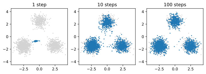
pred_v = make_pred(ema_v, linear, 'velocity')
samples = [ode_sample(pred_v, x_T, linear.sigma_bars(steps))
           for steps in (1, 10, 100)]
print('one step: mean', [round(v, 3) for v in samples[0].mean(0).tolist()],
      'std', [round(v, 3) for v in samples[0].std(0).tolist()])
for steps, x in zip((10, 100), samples[1:]):
    print(f'{steps} steps:', mix.summary(x))
print('largest difference to the loop:',
      float(jnp.abs(samples[2] - euler(ema_v, x_T, 100)).max()))
key, k_data = jax.random.split(key)
d2l.scatter_panels(samples, ['1 step', '10 steps', '100 steps'],
                   data=mix.sample(k_data, 2000));
one step: mean [-0.508, -0.699] std [0.039, 0.032]
10 steps: {'weights': [0.51, 0.296, 0.194], 'stray': 0.031, 'spread': 0.439}
100 steps: {'weights': [0.497, 0.304, 0.2], 'stray': 0.015, 'spread': 0.459}
largest difference to the loop: 0.0007569789886474609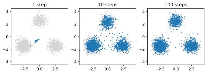
One step lands every start on the data mean \((-0.5, -0.7)\), with almost no spread, as the point-mass argument predicts. Ten steps recover the three modes with weights within about \(0.03\) of the targets, but about three percent of the samples stray between the modes. A hundred steps bring the strays down to about one percent, and the library’s sampler agrees with the loop to within \(10^{-3}\). The extra steps follow the curvature of the marginal flow.
17.2.3.2 The Reverse SDE and the Ancestral Chain
DDPM runs the reverse chain of Figure 17.2.2 instead, one stochastic step at a time. The reversal of a small forward step is nearly Gaussian (Sohl-Dickstein et al. 2015), and given the clean point it is exactly Gaussian: for \(s < t\), \(q(\mathbf{x}_s \mid \mathbf{x}_t, \mathbf{x}_0)\) has a mean linear in \(\mathbf{x}_t\) and \(\mathbf{x}_0\). Ho et al.’s ancestral step replaces \(\mathbf{x}_0\) by \(\hat{\mathbf{x}}_0\) in that mean and adds fresh noise with the variance \(\beta = 1 - \bar\alpha_t / \bar\alpha_s\) of the forward step. On the VP path, written with the score, it reads
\[ \mathbf{x}_s = \frac{\mathbf{x}_t + \beta\, \nabla \log p_t(\mathbf{x}_t)}{\sqrt{1 - \beta}} + \sqrt{\beta}\, \mathbf{z}, \qquad \mathbf{z} \sim \mathcal{N}(\mathbf{0}, \mathbf{I}). \tag{17.2.12}\]
With \(1/\sqrt{1 - \beta} \approx 1 + \beta/2\), the step splits to first order into two:
\[ \mathbf{x}_s \approx \Big[ \mathbf{x}_t + \tfrac{\beta}{2} \nabla \log p_t(\mathbf{x}_t) + \sqrt{\beta}\, \mathbf{z} \Big] + \tfrac{\beta}{2} \big( \mathbf{x}_t + \nabla \log p_t(\mathbf{x}_t) \big). \]
The bracket is a Langevin step of size \(h = \beta\), which leaves \(p_t\) in place and pulls stray points back toward it, and the second term is one Euler step of the probability-flow ODE from \(t\) back to \(s\), since on the VP path \(\mathbf{u}_t = -\tfrac12 \beta(t)\, (\mathbf{x} + \nabla \log p_t)\) and \(\beta \approx \beta(t)\, (t - s)\).
In continuous time the reversal is exact, by a theorem of Anderson (1982) . A forward process \(d\mathbf{x} = \mathbf{f}\, dt + g\, d\mathbf{W}\) is reversed, from \(t = 1\) down to \(0\), by
\[ d\mathbf{x} = \big[ \mathbf{f} - g^2 \nabla \log p_t(\mathbf{x}) \big]\, dt + g\, d\bar{\mathbf{W}}, \qquad\textrm{which has the same marginals as}\qquad \frac{d\mathbf{x}}{dt} = \mathbf{f} - \tfrac12 g^2 \nabla \log p_t(\mathbf{x}), \tag{17.2.13}\]
where \(\bar{\mathbf{W}}\) is a Brownian motion run backward. For the VP path, \(\mathbf{f} = -\tfrac12 \beta(t)\mathbf{x}\) and \(g^2 = \beta(t)\), the right-hand ODE is the flow we just integrated, and the ancestral step is, to first order, the Euler–Maruyama step (Section 43.3.4.1) of the SDE. Between the two lies a family of samplers with the same marginals: the more noise a sampler injects, the larger the score correction in its drift (Section 43.4.5, Figure 43.4.5).
ancestral_sample takes this step on any path with any predictor pred(x, alpha, sigma) -> (x0, eps), with the noise variance \(\sigma_t^2 - (\alpha_t/\alpha_s)^2 \sigma_s^2\) of the forward step from \(s\) to \(t\).
@torch.no_grad()
def ancestral_sample(pred, x, path, steps, *, t_start=1.0):
    """Ho et al.'s sampler from x at t_start (1 is noise) to data at t = 0."""
    a, s = path.grid(steps, t_start)
    for i in range(steps):
        x0, eps = pred(x, a[i], s[i])
        ratio = s[i + 1] * a[i] / (a[i + 1] * s[i])
        x = a[i + 1] * x0 + s[i + 1] * ratio * eps      # the posterior mean
        if s[i + 1] > 0:                                # no noise at t = 0
            var = s[i] ** 2 - (a[i] / a[i + 1] * s[i + 1]) ** 2  # forward step
            x = x + math.sqrt(var) * torch.randn_like(x)
    return x
def ancestral_sample(pred, x, path, steps, key, *, t_start=1.0):
"""Ho et al.'s sampler from x at t_start (1 is noise) to data at t = 0."""
a, s = path.grid(steps, t_start)
a_t, s_t, a_s, s_s = a[:-1], s[:-1], a[1:], s[1:]
ratio = s_s * a_t / (a_s * s_t)
var = jnp.maximum(s_t ** 2 - (a_t / a_s * s_s) ** 2, 0) # forward step
noise = jnp.where(s_s > 0, jnp.sqrt(var), 0) # none at t = 0
def step(x, inputs):
a_t, s_t, a_s, c_eps, c_noise, key = inputs
x0, eps = pred(x, a_t, s_t)
x = a_s * x0 + c_eps * eps # the posterior mean
return x + c_noise * jax.random.normal(key, x.shape), None
return jax.lax.scan(step, x, (a_t, s_t, a_s, s_s * ratio, noise,
jax.random.split(key, steps)))[0]We run two hundred steps of the chain with the noise model, from the same \(2{,}000\) starts as the flow.
pred_eps = make_pred(ema_eps, vp, 'eps')
print(mix.summary(ancestral_sample(pred_eps, x_T, vp, 200)))
{'weights': [0.515, 0.297, 0.189], 'stray': 0.0145, 'spread': 0.487}pred_eps = make_pred(ema_eps, vp, 'eps')
key, k_anc = jax.random.split(key)
print(mix.summary(ancestral_sample(pred_eps, x_T, vp, 200, k_anc))){'weights': [0.485, 0.311, 0.205], 'stray': 0.0105, 'spread': 0.478}The chain recovers the three modes with the right weights, up to the sampling error of \(2{,}000\) points, and about as few strays as the flow at a hundred steps; Ho et al. (2020) ran a thousand steps, but in two dimensions two hundred suffice. Either sampler can use either network through make_pred.
17.2.4 Experiments on the Running Example
Neither network ever saw the exact posterior. We compare each with the oracle in its predictions, its samples, and through the dictionary.
17.2.4.1 The Learned Predictor against the Optimal One
The loss of any predictor splits into the floor and a gap that training can still reduce, \(\mathbb{E}\|\boldsymbol\epsilon - \hat{\boldsymbol\epsilon}_{\boldsymbol\theta}\|^2 = \mathbb{E}\|\boldsymbol\epsilon - \boldsymbol\epsilon^\star\|^2 + \mathbb{E}\|\hat{\boldsymbol\epsilon}_{\boldsymbol\theta} - \boldsymbol\epsilon^\star\|^2\), with \(\boldsymbol\epsilon^\star\) the oracle’s noise prediction. We evaluate all three for the noise model on \(20{,}000\) fresh points at four times of the VP path.
def sq(u, w):
    """Mean squared distance between two batches of points."""
    return ((u - w) ** 2).sum(1).mean().item()

torch.manual_seed(4)
x0, eps = mix.sample(20_000), torch.randn(20_000, 2, device=device)
print('   t     gap   floor    loss')
with torch.no_grad():
    for t in (0.1, 0.3, 0.5, 0.7):
        tt = torch.full((len(x0),), t, device=device)
        x = vp.sample(x0, tt, eps)
        eps_hat = ema_eps(x, tt)
        eps_star = oracle(x, vp.alpha(tt), vp.sigma(tt))[1]
        print(f'{t:4} {sq(eps_hat, eps_star):7.4f} {sq(eps, eps_star):7.4f}'
              f' {sq(eps, eps_hat):7.4f}')
t gap floor loss
0.1 0.0004 1.3627 1.3625
0.3 0.0003 0.7730 0.7736
0.5 0.0001 0.4736 0.4736
0.7 0.0000 0.0540 0.0540def sq(u, w):
"""Mean squared distance between two batches of points."""
return float(((u - w) ** 2).sum(1).mean())
key, k_x0, k_eps = jax.random.split(key, 3)
x0, eps = mix.sample(k_x0, 20_000), jax.random.normal(k_eps, (20_000, 2))
print(' t gap floor loss')
for t in (0.1, 0.3, 0.5, 0.7):
tt = jnp.full((len(x0),), t)
x = vp.sample(x0, tt, eps)
eps_hat = ema_eps(x, tt)
eps_star = oracle(x, vp.alpha(tt), vp.sigma(tt))[1]
print(f'{t:4} {sq(eps_hat, eps_star):7.4f} {sq(eps, eps_star):7.4f}'
f' {sq(eps, eps_hat):7.4f}') t gap floor loss
0.1 0.0005 1.3544 1.3553
0.3 0.0003 0.7714 0.7717
0.5 0.0001 0.4759 0.4760
0.7 0.0000 0.0542 0.0543The loss column equals the floor plus the gap, to within the Monte Carlo error. The gap is below a thousandth at every time, on a target with unit variance per coordinate, and small next to the floor at every printed time: the network is close to the oracle wherever the data put their mass.
17.2.4.2 Samples from Both Samplers
A sampler accumulates the errors of all its steps. We draw \(20{,}000\) samples with two hundred ancestral steps of the noise model and a hundred Euler steps of the velocity model, and repeat both with the oracle in place of the network. At this sample size a mode weight carries a standard error of about \(0.0035\).
torch.manual_seed(5)
x_T = torch.randn(20_000, 2, device=device)
runs = {'data': mix.sample(20_000),
        'ancestral, network': ancestral_sample(pred_eps, x_T, vp, 200),
        'ancestral, oracle': ancestral_sample(oracle, x_T, vp, 200),
        'Euler, network': ode_sample(pred_v, x_T, linear.sigma_bars(100)),
        'Euler, oracle': ode_sample(oracle, x_T, linear.sigma_bars(100))}
for name, x in runs.items():
    print(f'{name:>18}:', mix.summary(x))
d2l.scatter_panels([runs[k][:2000] for k in runs],
                   list(runs), lim=4.5, size=2.4);
data: {'weights': [0.504, 0.299, 0.197], 'stray': 0.0103, 'spread': 0.476}
ancestral, network: {'weights': [0.503, 0.298, 0.199], 'stray': 0.0139, 'spread': 0.487}
ancestral, oracle: {'weights': [0.503, 0.301, 0.196], 'stray': 0.011, 'spread': 0.483}
Euler, network: {'weights': [0.5, 0.304, 0.197], 'stray': 0.0131, 'spread': 0.471}
Euler, oracle: {'weights': [0.499, 0.304, 0.197], 'stray': 0.0107, 'spread': 0.474}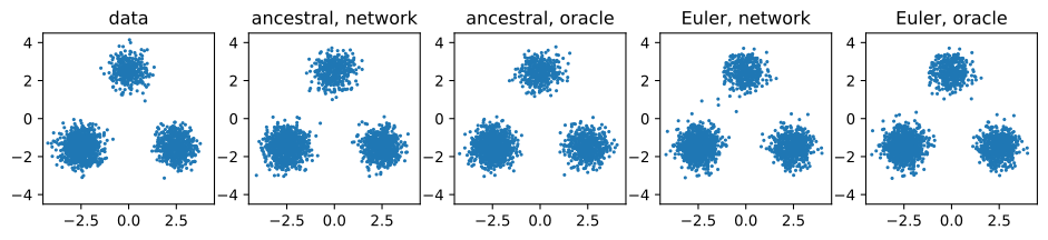
key, k_T, k_data, k_net, k_oracle = jax.random.split(key, 5)
x_T = jax.random.normal(k_T, (20_000, 2))
runs = {'data': mix.sample(k_data, 20_000),
        'ancestral, network': ancestral_sample(pred_eps, x_T, vp, 200, k_net),
        'ancestral, oracle': ancestral_sample(oracle, x_T, vp, 200, k_oracle),
        'Euler, network': ode_sample(pred_v, x_T, linear.sigma_bars(100)),
        'Euler, oracle': ode_sample(oracle, x_T, linear.sigma_bars(100))}
for name, x in runs.items():
    print(f'{name:>18}:', mix.summary(x))
d2l.scatter_panels([runs[k][:2000] for k in runs],
                   list(runs), lim=4.5, size=2.4);
data: {'weights': [0.503, 0.298, 0.199], 'stray': 0.0094, 'spread': 0.478}
ancestral, network: {'weights': [0.497, 0.3, 0.203], 'stray': 0.0124, 'spread': 0.485}
ancestral, oracle: {'weights': [0.499, 0.298, 0.203], 'stray': 0.0134, 'spread': 0.485}
Euler, network: {'weights': [0.495, 0.308, 0.197], 'stray': 0.0117, 'spread': 0.47}
Euler, oracle: {'weights': [0.495, 0.307, 0.198], 'stray': 0.0106, 'spread': 0.472}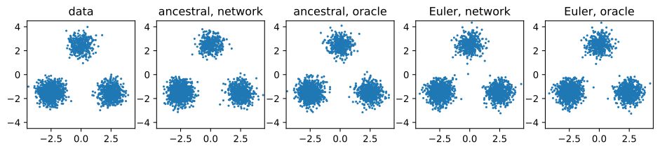
The ancestral chain with the network recovers the weights \(0.5/0.3/0.2\) within sampling error, and Euler with the network matches them to within about \(0.01\). Every sampler, network or oracle, strays about as often as the data themselves, about one percent, the share of a Gaussian beyond three standard deviations. Both samplers recover the mode weights, which no single noise level could.
17.2.4.3 The Dictionary Checked
If both networks learned the posterior mean, each should match the linear-path velocity that Equation 17.2.9 computes from the exact score of \(p_t\) (mix.score with \(\alpha = 1 - t\) and \(\sigma = t\)). For the noise model, make_pred returns \((\hat{\mathbf{x}}_0, \hat{\boldsymbol\epsilon})\), whose difference is the linear-path velocity. We stop at \(t = 0.95\), because a noise model has no clean-point estimate at \(\alpha = 0\).
print('   t  E|u|^2  velocity net  noise net')
with torch.no_grad():
    for t in (0.2, 0.5, 0.8, 0.95):
        tt = torch.full((len(x0),), t, device=device)
        x = linear.sample(x0, tt, eps)
        u = -(x + t * mix.score(x, 1 - t, t)) / (1 - t)  # from the score
        x0_hat, eps_hat = pred_eps(x, 1 - t, t)
        print(f'{t:4} {sq(u, 0):7.2f} {sq(ema_v(x, tt), u):13.4f}'
              f' {sq(eps_hat - x0_hat, u):10.4f}')
t E|u|^2 velocity net noise net
0.2 8.05 0.0003 0.0005
0.5 7.74 0.0007 0.0016
0.8 1.07 0.0009 0.0017
0.95 2.00 0.0005 0.0136print(' t E|u|^2 velocity net noise net')
for t in (0.2, 0.5, 0.8, 0.95):
tt = jnp.full((len(x0),), t)
x = linear.sample(x0, tt, eps)
u = -(x + t * mix.score(x, 1 - t, t)) / (1 - t) # from the score
x0_hat, eps_hat = pred_eps(x, 1 - t, t)
print(f'{t:4} {sq(u, 0):7.2f} {sq(ema_v(x, tt), u):13.4f}'
f' {sq(eps_hat - x0_hat, u):10.4f}') t E|u|^2 velocity net noise net
0.2 8.05 0.0004 0.0006
0.5 7.73 0.0014 0.0013
0.8 1.07 0.0011 0.0016
0.95 2.00 0.0006 0.0133The velocity network differs from the field computed from the score by less than a quarter of a percent of the field’s mean squared norm, which ranges from about \(8\) at \(t = 0.2\) to about \(1\) at \(t = 0.8\). The noise network, converted through two paths and a change of time, stays within about one percent, with its largest error at \(t = 0.95\), where the conversion divides by a small \(\alpha\). No score was learned, and no velocity appears in the noise model’s loss.
17.2.5 Summary
A Gaussian path connects the data to noise through every noise level, and a walk down it settles the mode weights at coarse levels and the details at fine ones. One regression onto per-example targets trains one network along the whole path, because least squares recovers the posterior mean; the score, noise, clean point, \(v\) and velocity are affine functions of it, and the models of the literature differ only in path, target and sampler (Table 17.2.1). Samples come from the probability-flow ODE or the ancestral chain. On the mixture both learned models sit at their loss floors, agree through the dictionary, and recover the mode weights.
| model | target and path | sampler | where |
|---|---|---|---|
| denoising score model | the noise, at one level | Langevin dynamics | Section 17.1 |
| noise-conditional score network | the noise at each level of a ladder, weighted by \(\tilde\sigma^2\) | annealed Langevin dynamics | here, 10 |
| DDPM | \(\boldsymbol\epsilon\) on the VP path | the ancestral chain or the probability-flow ODE | here, Section 17.3 |
| flow matching, rectified flow | \(\boldsymbol\epsilon - \mathbf{x}_0\) on the linear path | Euler steps on the probability-flow ODE | here, Section 17.4 |
| \(\mathbf{v}\)-prediction | \(\mathbf{v}\) on the cosine path | either, through the dictionary | Section 17.5 |
| masked diffusion | the clean tokens of a partly masked sequence, by a weighted cross-entropy | iterative unmasking | Section 17.8 |
Nothing in this section used the fact that \(\mathbf{x}\) had two coordinates. An image has thousands, and its pixels are strongly correlated; the next question is what network, and what changes to training and sampling, a path through image space needs.
17.2.6 Exercises
- The marginal of the linear path. The linear path Equation 17.2.2 joins a draw \(\mathbf{x}_0\) of the mixture, with weights \(\pi_k\), means \(\boldsymbol\mu_k\) and standard deviation \(s = 0.5\) per coordinate, to independent noise \(\boldsymbol\epsilon\).
- Show that \(p_t\) is the mixture with weights \(\pi_k\), means \((1 - t)\boldsymbol\mu_k\) and per-coordinate variance \((1 - t)^2 s^2 + t^2\). Derive Equation 17.2.9 from Equation 17.2.8.
- Show from Equation 17.2.5 that \(\mathbf{u}_t(\mathbf{x}) \to \mathbf{x} - \mathbb{E}[\mathbf{x}_0]\) as \(t \to 1\), and conclude where one Euler step from \(t = 1\) to \(t = 0\) sends every start.
- With two Euler steps the first ends at \(t = 1/2\). Show that it maps \(\mathcal{N}(\mathbf{0}, \mathbf{I})\) to \(\mathcal{N}(\mathbb{E}[\mathbf{x}_0]/2, \mathbf{I}/4)\), and compare the center and the width of this cloud with those of \(p_{1/2}\). Which mode should the two-step samples overweight, and why?
- Velocity, noise and clean-point targets. On the linear path, take the posterior mean of \(\mathbf{x}_t = (1 - t)\mathbf{x}_0 + t\boldsymbol\epsilon\).
- Show that the marginal velocity equals both \((\mathbf{x} - \hat{\mathbf{x}}_0)/t\) and \((\hat{\boldsymbol\epsilon} - \mathbf{x})/(1 - t)\).
- By the first part, an error in \(\hat{\mathbf{x}}_0\) reaches the velocity divided by \(t\), and an error in \(\hat{\boldsymbol\epsilon}\) divided by \(1 - t\). Near which end of the path is each prediction a poor source of the velocity, and how does this explain why a noise model is never queried at \(\alpha = 0\)? (8 works out the propagation of errors between all targets on the cosine path.)
- Show that the velocity loss of \(\mathbf{u}_{\boldsymbol\theta} = (\mathbf{x} - \hat{\mathbf{x}}_{0,\boldsymbol\theta})/t\) equals the clean-point loss \(\mathbb{E}\|\hat{\mathbf{x}}_{0,\boldsymbol\theta} - \mathbf{x}_0\|^2\) weighted by \(1/t^2\), and the velocity loss of \(\mathbf{u}_{\boldsymbol\theta} = (\hat{\boldsymbol\epsilon}_{\boldsymbol\theta} - \mathbf{x})/(1 - t)\) equals the noise loss weighted by \(1/(1 - t)^2\). Which times does flow matching emphasize relative to each of the two unweighted losses?
- [code] The loss floor. Use
oracleandloss_floor.- Plot the floor of the velocity target on the linear path and of the noise target on the VP path against \(t\) on a grid in \((0, 1)\). Where is each largest? The printed training loss is a mean over \(1{,}000\) minibatches of \(512\) points; estimate its standard error from
losses_v, and decide whether a printed loss below the floor would be a contradiction. - Let \(\boldsymbol\Sigma\) be the covariance matrix of the mixture, with eigenvalues \(\kappa_1, \kappa_2\). For Gaussian data with this covariance, show that the velocity floor on the linear path at time \(t\) is \(\sum_i \kappa_i / \big((1 - t)^2 \kappa_i + t^2\big)\). Add this curve to the plot, and explain why it cannot lie below the floor of the mixture. Why do the two floors agree at both ends of the path?
- The score target \(-\boldsymbol\epsilon/\sigma_t\) has the floor of the noise target divided by \(\sigma_t^2\). Evaluate it on the VP path at \(t = 0.01\), \(0.1\) and \(0.5\), and explain why no network is trained on this target with \(t\) uniform on \((0, 1)\).
- The noise model’s training loss is about a tenth of the velocity model’s. Is it the better model? Wrap
ema_epsandema_vwithmake_pred, and at the noise levels of the linear path at \(t \in \{0.1, 0.5, 0.9\}\) measure each network’s gap to the oracle in a common unit, \(\mathbb{E}\|\hat{\mathbf{x}}_0 - \hat{\mathbf{x}}_0^\star\|^2\), where \(\hat{\mathbf{x}}_0^\star\) comes fromoracle. Use the weights of Exercise 2c, and the factor \(\alpha_t^2/\sigma_t^2\) that turns a clean-point error into a noise error, to explain why the raw losses differ so much. Which comparison ranks the two models: the raw losses, or each loss’s excess over its own floor?
- Plot the floor of the velocity target on the linear path and of the noise target on the VP path against \(t\) on a grid in \((0, 1)\). Where is each largest? The printed training loss is a mean over \(1{,}000\) minibatches of \(512\) points; estimate its standard error from
- The ancestral step to first order, for Gaussian data. ● Let the data be \(\mathcal{N}(\mathbf{0}, s^2 \mathbf{I})\), so that on the DDPM chain \(q_k = \mathcal{N}(\mathbf{0}, v_k \mathbf{I})\) with \(v_k = \bar\alpha_k s^2 + 1 - \bar\alpha_k\).
- Show that one ancestral step Equation 17.2.12 with the exact score and step variance \(\beta_k\) maps \(q_k\) to \(\mathcal{N}\big(\mathbf{0}, (v_{k-1} + \delta_k)\mathbf{I}\big)\) with \(\delta_k = \beta_k^2 (1/v_k - 1)/(1 - \beta_k)\).
- For which data is the step exact? Is the variance too large or too small for data narrower than the standard Gaussian, such as one component of the mixture, \(s = 0.5\)?
- How does the error accumulated over the chain change when the schedule is refined to twice as many steps with half the \(\beta_k\)?
- Step size and Gaussian reversal. ● The ancestral chain uses Gaussian transitions, which are justified for small steps. This problem measures how small. Write \(\sigma_{t|s}^2 = \sigma_t^2 - (\alpha_t/\alpha_s)^2 \sigma_s^2\) for the variance of the forward step from \(s\) to \(t > s\).
- Show that the exact reversal is the mixture \(q(\mathbf{x}_s \mid \mathbf{x}_t) = \mathbb{E}_{\mathbf{x}_0 \mid \mathbf{x}_t}\big[q(\mathbf{x}_s \mid \mathbf{x}_t, \mathbf{x}_0)\big]\) and that its covariance is \(\tau^2 \mathbf{I} + c^2\, \textrm{Cov}[\mathbf{x}_0 \mid \mathbf{x}_t]\), where \(\tau^2 = \sigma_{t|s}^2 \sigma_s^2/\sigma_t^2\) is the variance of \(q(\mathbf{x}_s \mid \mathbf{x}_t, \mathbf{x}_0)\) and \(c = \alpha_s \sigma_{t|s}^2/\sigma_t^2\) is the coefficient of \(\mathbf{x}_0\) in its mean.
- Let the data be \(\pm 1\) with equal probability in one dimension, and let \(x_t = 0\). Show that the reversal is the equal mixture of \(\mathcal{N}(\pm c, \tau^2)\), which is bimodal exactly when \(\zeta^2 = c^2/\tau^2\) exceeds one, and that \(\zeta^2 = \alpha_s^2 \sigma_{t|s}^2 / (\sigma_t^2 \sigma_s^2)\). How does \(\zeta\) shrink as the step \(t - s\) is refined?
- Evaluate \(\zeta\) on the VP path from \(t = 0.5\) to \(s = 0.495\), \(0.45\) and \(0.3\), and for one step from \(t = 0.3\) to \(s = 0\). Which reversals are bimodal? What does a Gaussian transition with the optimal mean produce at \(x_t = 0\) in the last case, and what should it produce?
- [code] Commitment time. ● When along the path does a sample decide its mode? Biroli et al. (2024) measure this by cloning: start at a point of \(q_t\), run two copies of the reverse chain with independent noise, and record whether they end in the same mode.
- Draw \(2{,}000\) clean points, noise them to \(\mathbf{x}_t\) on the VP path for \(t = 0.9, 0.7, 0.5, 0.4, 0.3, 0.2, 0.1\), and run two copies of
ancestral_sample(pred_eps, x_t, vp, steps, t_start=t)from each with about \(200\, t\) steps. Plot the fraction \(\varphi(t)\) of pairs whose ends have the same nearest mean. Which value does \(\varphi\) approach as \(t \to 1\), and why? - Let \(\Lambda\) be the largest eigenvalue of the covariance of the data. Biroli et al. define the speciation time by \(\bar\alpha_t \Lambda = 1\), where the signal along the top principal direction stops dominating the noise. Compute it for the mixture and compare it with your curve and with the ladder of this section, whose coarse levels decided the mode weights. 3 and 6 work out the same question for two modes in one dimension.
- Draw \(2{,}000\) clean points, noise them to \(\mathbf{x}_t\) on the VP path for \(t = 0.9, 0.7, 0.5, 0.4, 0.3, 0.2, 0.1\), and run two copies of
- Same ratio, same flow. ● Let two Gaussian paths have coefficients related by \(\alpha^B_t = c_t\, \alpha^A_t\) and \(\sigma^B_t = c_t\, \sigma^A_t\) for a smooth positive function \(c_t\), so that they have the same log-SNR at every time.
- Show that \(p^B_t(\mathbf{y}) = c_t^{-d}\, p^A_t(\mathbf{y}/c_t)\), and use Equation 17.2.8 to show that \(\mathbf{u}^B_t(\mathbf{y}) = (\dot c_t / c_t)\, \mathbf{y} + c_t\, \mathbf{u}^A_t(\mathbf{y}/c_t)\). Conclude that the trajectories of the probability-flow ODE are related by \(\mathbf{y}_t = c_t\, \mathbf{x}_t\).
- Let \(\tau(t)\) be increasing. Show that the path \(p_{\tau(t)}\) is generated by the field \(\dot\tau(t)\, \mathbf{u}_{\tau(t)}\), with the same trajectories as \(\mathbf{u}\).
- Find the change of time \(\tau(t)\) for which the cosine path \((\cos\frac{\pi\tau}{2}, \sin\frac{\pi\tau}{2})\) at time \(\tau(t)\) has the log-SNR of the linear path at time \(t\), and show that \(c_t = 1/\sqrt{(1 - t)^2 + t^2}\). Where along the path is the rescaling largest?
- What does the probability-flow ODE of the cosine path do to data distributed as \(\mathcal{N}(\mathbf{0}, \mathbf{I})\), and why? What does that of the linear path do to the same data?
- Ladder spacing in high dimensions. ● Let the data be a single point at the origin of \(\mathbb{R}^d\), so that \(p_{\tilde\sigma} = \mathcal{N}(\mathbf{0}, \tilde\sigma^2 \mathbf{I})\), and let the ladder be geometric with ratio \(q = \tilde\sigma_{i-1}/\tilde\sigma_i > 1\).
- Show that \(r = \|\mathbf{x}\|\) for \(\mathbf{x} \sim p_{\tilde\sigma}\) satisfies \(\mathbb{E}[r^2] = d\tilde\sigma^2\) and \(\textrm{Var}[r^2] = 2d\tilde\sigma^4\), and conclude that \(r\) is approximately \(\mathcal{N}(\tilde\sigma\sqrt d, \tilde\sigma^2/2)\) for large \(d\).
- A chain that leaves level \(i - 1\) with a sample of \(p_{\tilde\sigma_{i-1}}\) enters level \(i\) at a radius that lies, with high probability, in \(\tilde\sigma_{i-1}(\sqrt d \pm 3/\sqrt 2)\). Show that \(p_{\tilde\sigma_i}\) puts the mass \(\Phi\big(\sqrt{2d}(q - 1) + 3q\big) - \Phi\big(\sqrt{2d}(q - 1) - 3q\big)\) on this interval, where \(\Phi\) is the standard normal distribution function. Why does a mass near zero mean that the chain starts the level where the network has seen almost no training inputs?
- Song and Ermon (2020) choose \(q\) so that this mass is about one half. Solve for \(q\) at \(d = 3072\), the dimension of CIFAR-10 images, and count the levels from \(\tilde\sigma = 50\) down to \(0.01\). Compare with the \(232\) levels of their CIFAR-10 model.
- The top level must also be coarse enough to merge the modes. Two equal Gaussian components at \(\pm\mu\) with variance \(v\) have a single mode exactly when \(\mu^2 \le v\) (6). Use this criterion on the two lower modes of the mixture to estimate the noise level at which they merge, and compare it with the ladder’s top level of \(3\).
- [code] The exact optimum memorizes. A finite training set is itself a distribution, a mixture of point masses, and its exact velocity field is known. Bertrand et al. (2025) take as their starting point that integrating this field reproduces the training points, and ask why trained networks generalize instead.
- Draw \(64\) points from the mixture and train
TimeMLP(256, 3)withregression_loss(linear, 'velocity')on batches drawn from these points only. d2l.GaussianMixture(points, [1/64] * 64, 0.0)is the empirical distribution, and itsvelocitymethod is the exact field for \(t > 0\). Integrate it and the trained network witheulerfrom the same \(2{,}000\) starts. For both sets of samples, plot the histogram of the distance to the nearest training point.- Which sampler reproduces the training set, and which produces new points? Bertrand et al. argue that the noise in the regression targets is not what makes the network generalize. Repeat the first two parts with \(1{,}024\) training points, and describe how the two histograms change.
- Draw \(64\) points from the mixture and train
- [extended] A noise-conditional score network on the mixture. ●● Train the model of Song and Ermon (2019) on the running example and compare it with the samplers of this section.
- Train one
TimeMLPon the ten levels of the ladder, with the level’s log-noise \(\log\tilde\sigma_i\) as its time input, by denoising score matching weighted by \(\tilde\sigma_i^2\): the loss of level \(i\) is \(\mathbb{E}\|\tilde\sigma_i\, \mathbf{s}_{\boldsymbol\theta}(\mathbf{x}_0 + \tilde\sigma_i \boldsymbol\epsilon, \tilde\sigma_i) + \boldsymbol\epsilon\|^2\). Why does the weight make the levels comparable? - Run annealed Langevin dynamics with the learned scores, \(100\) steps per level as in the text, and compare the summary with the exact-score ladder.
- The ladder used \(1{,}000\) network evaluations. Compare it with
ancestral_sampleandode_sampleat the same number of evaluations, and with fewer. Which hand-chosen quantities of the ladder does the path make unnecessary?
- Train one