torch.set_float32_matmul_precision('high') # tf32 matmuls on tensor cores17.6 Latent Diffusion and Transformers
The image models of this chapter draw \(28 \times 28\) garments with a U-Net that processes every pixel at each of fifty sampling steps. The text-to-image systems that many readers have used draw pictures of a million pixels in seconds, and the papers behind most of them describe neither a U-Net nor a network that looks at pixels. The previous section hinted at the reason: most pixels carry detail that a viewer hardly notices. Why do current systems diffuse something other than pixels, why is their network a transformer, and how does a caption steer it?
Rombach et al. (2022) split generation into two stages. An autoencoder compresses each image into a small grid of numbers, its latent, from which a decoder restores the image with little visible loss, and a diffusion model learns the distribution of the latents at a fraction of the cost per step. Peebles and Xie (2023) replaced the U-Net by a transformer that reads the latent grid as a sequence of patches, the diffusion transformer (DiT), and found that its samples improve steadily as its computation grows.
Together the two ideas are the design of most recent image and video generators. We train a small autoencoder on Fashion-MNIST and run the regression of the previous sections on its latents, then build the DiT and train it at three sizes, and close with text and video, a paragraph each. Systems at full scale are the subject of a later part of this book.
17.6.1 Why a Latent Space
17.6.1.1 The Cost of Pixels
Every sampling step evaluates the network on the whole image. A convolution applies its kernel at every pixel, so the cost of a U-Net grows with the number of pixels; attention compares every position with every other, so its cost grows with their square. A \(512 \times 512\) color image holds \(512 \cdot 512 \cdot 3 = 786{,}432\) numbers.
Most of these numbers describe detail. In Section 17.5.3.2 the power of Fashion-MNIST images fell by three orders of magnitude from one to fourteen cycles per image, and the sampler fixed the silhouette of a garment at high noise and added its texture in the last steps. A viewer rarely notices a wrong texture, but a missing sleeve is obvious.
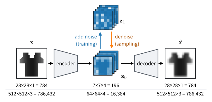
Rate–distortion theory makes this precise: for each level of distortion, the rate–distortion function gives the fewest bits per image that a code needs (Section 42.4.3.2). Rombach et al. (2022) observed that a likelihood model of natural images spends most of its bits on imperceptible details, at the low-distortion end of this curve. They leave this perceptual compression to an autoencoder, and the semantic compression, the modeling of what the image shows, to the diffusion model. The autoencoder of Stable Diffusion maps a \(512 \times 512 \times 3\) image to a \(64 \times 64 \times 4\) latent, 48 times fewer numbers. Every diffusion step works on the latent, and the decoder runs once per sample.
The latent must keep enough information for the decoder and be easy for the diffusion model to learn. A latent that stored every pixel would reconstruct perfectly and be as hard to model as the pixels; Dieleman (2025) calls this a trade between rate, distortion and modelability. Our autoencoder maps 784 numbers to a \(7 \times 7\) grid with four channels, 196 numbers (Figure 17.6.1).
17.6.1.2 The Autoencoder
A latent is easy to model if it has a known scale, against which the noise of the Gaussian path is calibrated, if it has no isolated outliers, and if nearby latents decode to similar images, so that a slightly wrong latent still gives a plausible image. An autoencoder trained only to reconstruct guarantees none of this.
The variational autoencoder (Kingma and Welling 2014) supplies the remedy. The encoder outputs a mean \(\boldsymbol\mu\) and a standard deviation \(\mathbf{s}\) for each of the 196 latent numbers, the latent is drawn as \(\mathbf{z} = \boldsymbol\mu + \mathbf{s} \odot \boldsymbol\xi\) with standard normal \(\boldsymbol\xi\), and the decoder maps \(\mathbf{z}\) to a reconstruction \(\hat{\mathbf{x}}\). The loss adds to the reconstruction error a term that pulls each latent number toward a standard normal:
\[\mathcal{L}(\mathbf{x}) = \frac{1}{784}\,\|\mathbf{x} - \hat{\mathbf{x}}\|^2 + \frac{\beta}{196} \sum_{j=1}^{196} \tfrac{1}{2}\left(\mu_j^2 + s_j^2 - 1 - \log s_j^2\right). \tag{17.6.1}\]
The sum is the Kullback–Leibler divergence from \(\mathcal{N}(\boldsymbol\mu, \mathrm{diag}(\mathbf{s}^2))\) to \(\mathcal{N}(\mathbf{0}, \mathbf{I})\), the term of the evidence lower bound (Section 41.5.5), and \(\beta\) is its weight (not the schedule’s \(\beta_k\)). With \(\beta = 10^{-4}\) the reconstruction stays in charge, and the KL term only stops the encoder from inflating its means or shrinking its standard deviations to zero. The autoencoders of large systems add a patch critic and a perceptual loss, because a squared error averages plausible textures into a blur (Section 16.7); others quantize the latent into discrete tokens (Esser et al. 2021; Chang et al. 2022).
Our autoencoder stacks the residual blocks of the U-Net, without an embedding, at widths 64 and 128; its encoder halves the resolution twice to a \(7 \times 7\) grid with a mean and a log variance per latent channel, and its decoder mirrors it.
class Autoencoder(nn.Module):
    """Residual convolutional autoencoder from 28x28x1 images to a 7x7
    Gaussian latent and back; returns the reconstruction and the KL term."""
    def __init__(self, latent_channels=4, ch=64, num_blocks=2):
        super().__init__()
        blocks = lambda a, b: [d2l.UNetBlock(a, b)] + [
            d2l.UNetBlock(b, b) for _ in range(num_blocks - 1)]
        down = lambda c: nn.Conv2d(c, c, 3, stride=2, padding=1)
        head = lambda a, b: [nn.GroupNorm(8, a), nn.SiLU(),
                             nn.Conv2d(a, b, 3, padding=1)]
        self.encoder = nn.Sequential(
            nn.Conv2d(1, ch, 3, padding=1), *blocks(ch, ch),
            down(ch), *blocks(ch, 2 * ch),                       # 14 x 14
            down(2 * ch), *blocks(2 * ch, 2 * ch),               # 7 x 7
            *head(2 * ch, 2 * latent_channels))  # mean and log variance
        self.decoder = nn.Sequential(
            nn.Conv2d(latent_channels, 2 * ch, 3, padding=1),
            *blocks(2 * ch, 2 * ch),
            nn.Upsample(scale_factor=2), *blocks(2 * ch, ch),    # 14 x 14
            nn.Upsample(scale_factor=2), *blocks(ch, ch),        # 28 x 28
            *head(ch, 1))

    def encode(self, x):
        mean, log_var = self.encoder(x).chunk(2, dim=1)
        return mean, log_var.clamp(-30, 20)

    def forward(self, x):
        mean, log_var = self.encode(x)
        z = mean + (0.5 * log_var).exp() * torch.randn_like(mean)
        kl = 0.5 * (mean ** 2 + log_var.exp() - 1 - log_var).mean()
        return self.decoder(z), kl
class Autoencoder(nnx.Module):
"""Residual convolutional autoencoder from 28x28x1 images to a 7x7
Gaussian latent and back; returns the reconstruction and the KL term."""
def __init__(self, latent_channels=4, ch=64, num_blocks=2, *, rngs):
blocks = lambda a, b: [d2l.UNetBlock(a, b, rngs=rngs)] + [
d2l.UNetBlock(b, b, rngs=rngs) for _ in range(num_blocks - 1)]
conv = lambda a, b, **kw: d2l.Conv(a, b, (3, 3), rngs=rngs, **kw)
down = lambda c: conv(c, c, strides=2, padding=1)
up = lambda x: jnp.repeat(jnp.repeat(x, 2, axis=1), 2, axis=2)
head = lambda a, b: [nnx.GroupNorm(a, num_groups=8, epsilon=1e-5,
use_fast_variance=False,
rngs=rngs), nnx.silu, conv(a, b)]
self.encoder = nnx.Sequential(
conv(1, ch), *blocks(ch, ch),
down(ch), *blocks(ch, 2 * ch), # 14 x 14
down(2 * ch), *blocks(2 * ch, 2 * ch), # 7 x 7
*head(2 * ch, 2 * latent_channels)) # mean and log variance
self.decoder = nnx.Sequential(
conv(latent_channels, 2 * ch), *blocks(2 * ch, 2 * ch),
up, *blocks(2 * ch, ch), # 14 x 14
up, *blocks(ch, ch), # 28 x 28
*head(ch, 1))
def encode(self, x):
mean, log_var = jnp.split(self.encoder(x), 2, axis=-1)
return mean, jnp.clip(log_var, -30, 20)
def __call__(self, x, key):
mean, log_var = self.encode(x)
z = mean + jnp.exp(0.5 * log_var) * jax.random.normal(key, mean.shape)
kl = 0.5 * (mean ** 2 + jnp.exp(log_var) - 1 - log_var).mean()
return self.decoder(z), klWe train it for 20,000 updates with d2l.train_regression of Section 17.1, which runs Adam on a loss and returns the trained model, a moving average of its weights and the losses. The learning rate decays to zero along a cosine, so the final weights need no averaging.
X, y, X_test, y_test = d2l.load_fashion_mnist_pm1()
dev = X.device

def batch_fn():
    return X[torch.randint(0, len(X), (128,), device=dev)]

def ae_loss(ae, x):
    x_hat, kl = ae(x)
    return ((x_hat - x) ** 2).mean() + 1e-4 * kl

torch.manual_seed(1)
ae, _, _ = d2l.train_regression(d2l.Autoencoder().to(dev), ae_loss, batch_fn,
                                20_000, cosine=True)
print(f'{d2l.num_params(ae) / 1e6:.2f}M parameters')
2.40M parametersX, y, X_test, y_test = d2l.load_fashion_mnist_pm1()
def batch_fn(key):
return X[jax.random.randint(key, (128,), 0, len(X))]
def ae_loss(ae, x, key):
x_hat, kl = ae(x, key)
return ((x_hat - x) ** 2).mean() + 1e-4 * kl
ae, _, _ = d2l.train_regression(d2l.Autoencoder(rngs=nnx.Rngs(1)), ae_loss,
batch_fn, 20_000, jax.random.key(1),
cosine=True)
print(f'{d2l.num_params(ae) / 1e6:.2f}M parameters')2.40M parametersThe first row shows eight test images, the second the decoder’s output for their latent means.
with torch.no_grad():
    x_hat = ae.decoder(ae.encode(X_test[:8])[0])
d2l.show_gray(torch.cat([X_test[:8], x_hat]), 2, 8);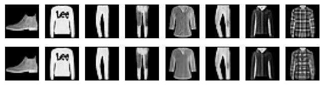
encode = nnx.jit(lambda ae, x: ae.encode(x))      # mean and log variance
decoder = nnx.jit(lambda ae, z: ae.decoder(z))
x_hat = decoder(ae, encode(ae, X_test[:8])[0])
d2l.show_gray(jnp.concatenate([X_test[:8], x_hat]), 2, 8);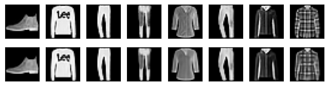
The reconstructions are hard to tell from the originals. To measure them we use the Fréchet distance (FD) of Section 17.3, the distance between Gaussians fitted to the features that a small classifier, d2l.FeatureCNN, extracts from two sets of images. Two sets of real images differ by chance too, so we print the FD between two disjoint sets of 5,000 test images as the floor. All FDs in this section use 5,000 images; at 1,000 the floor is about six times higher.
cnn = d2l.fashion_feature_cnn(X, y)
f_ref = d2l.fd_features(cnn, X_test[:5000])

def fd(imgs):
    """FD of images against the first 5,000 test images."""
    return d2l.fid_score(d2l.fd_features(cnn, imgs), f_ref)

print(f'floor, the other 5,000 test images: FD {fd(X_test[5000:]):.2f}')
floor, the other 5,000 test images: FD 0.17cnn = d2l.fashion_feature_cnn(X, y)
f_ref = d2l.fd_features(cnn, X_test[:5000])
def fd(imgs):
"""FD of images against the first 5,000 test images."""
return d2l.fid_score(d2l.fd_features(cnn, imgs), f_ref)
print(f'floor, the other 5,000 test images: FD {fd(X_test[5000:]):.2f}')floor, the other 5,000 test images: FD 0.18We score the reconstructions of the other 5,000 test images.
x_hat = d2l.batched(lambda x: ae.decoder(ae.encode(x)[0]), X_test[5000:])
fd_rec = fd(x_hat)
print(f'reconstructions: squared error {((x_hat - X_test[5000:]) ** 2).mean():.4f}'
      f' per pixel, FD {fd_rec:.2f}')
reconstructions: squared error 0.0038 per pixel, FD 0.65x_hat = d2l.batched(lambda x: decoder(ae, encode(ae, x)[0]), X_test[5000:])
fd_rec = fd(x_hat)
print(f'reconstructions: squared error {((x_hat - X_test[5000:]) ** 2).mean():.4f}'
f' per pixel, FD {fd_rec:.2f}')reconstructions: squared error 0.0039 per pixel, FD 0.78The reconstructions score an FD of 0.6 to 0.8 against the floor of 0.17, at a squared error of about 0.004 per pixel. This bounds every latent model trained with this autoencoder: perfect latents would decode to reconstructions and score the same.
We encode the training set once and print the standard deviation of the latents, the average of the encoder’s \(\mathbf{s}\), and the excess kurtosis of all latent values, which is zero for a normal distribution and large when a few values lie far out.
encoded = d2l.batched(lambda x: torch.cat(ae.encode(x), 1), X)
mu, log_var = encoded.chunk(2, dim=1)       # mean and log variance
s = (0.5 * log_var).exp()
z = mu + s * torch.randn_like(mu)
scale = 1 / z.std().item()
kurtosis = (((z - z.mean()) * scale) ** 4).mean() - 3
print(f'latent std {z.std():.2f} (scale factor {scale:.2f}), encoder std '
      f'{s.mean():.3f}, excess kurtosis {kurtosis:.2f}')
latent std 0.94 (scale factor 1.07), encoder std 0.026, excess kurtosis -0.21encoded = d2l.batched(lambda x: jnp.concatenate(encode(ae, x), -1), X)
mu, log_var = jnp.split(encoded, 2, axis=-1) # mean and log variance
s = jnp.exp(0.5 * log_var)
z = mu + s * jax.random.normal(jax.random.key(2), mu.shape)
scale = 1 / float(z.std())
kurtosis = (((z - z.mean()) * scale) ** 4).mean() - 3
print(f'latent std {z.std():.2f} (scale factor {scale:.2f}), encoder std '
f'{s.mean():.3f}, excess kurtosis {kurtosis:.2f}')latent std 0.95 (scale factor 1.05), encoder std 0.024, excess kurtosis -0.47The latents have a standard deviation slightly below one, so we multiply them by a factor \(c\) of about 1.05. The encoder’s standard deviation is 0.02 to 0.03, so the KL term barely blurs each code, and the excess kurtosis is near zero or negative: the latents have no heavy tails. A larger \(\beta\) makes them closer to normal but costs reconstruction quality (7).
17.6.2 Diffusion in the Latent Space
17.6.2.1 The Same Regression on Latents
With the autoencoder fixed, nothing changes but the data. Each batch draws the latents of 128 training images, \(\mathbf{z}_0 = c\,(\boldsymbol\mu + \mathbf{s} \odot \boldsymbol\xi)\), fresh from the encoder’s distribution as Rombach et al. (2022) do. We train on the linear path of Section 17.2: we form \(\mathbf{z}_t = (1 - t)\,\mathbf{z}_0 + t\,\boldsymbol\epsilon\) and regress the network’s output onto the velocity \(\boldsymbol\epsilon - \mathbf{z}_0\).
The scale factor matters because the path mixes the data with noise of unit variance. Latents with a standard deviation of five would shift the log-SNR at every time by \(\log 25\) (1), and Stable Diffusion multiplies its latents by 0.18215 for this reason. The network is the U-Net of Section 17.3 with four input and output channels, and one loss_fn serves images and latents.
path = d2l.GaussianPath.linear()
loss_fn = d2l.regression_loss(path, 'velocity')  # for images or latents

def latent_batch_fn():
    i = torch.randint(0, len(mu), (128,), device=dev)
    return (mu[i] + s[i] * torch.randn_like(mu[i])) * scale

torch.manual_seed(3)
_, unet_latent, _ = d2l.train_regression(
    d2l.UNet(ch=64, in_channels=4, out_channels=4).to(dev), loss_fn,
    latent_batch_fn, 20_000)
path = d2l.GaussianPath.linear()
loss_fn = d2l.regression_loss(path, 'velocity') # for images or latents
def latent_batch_fn(key):
k1, k2 = jax.random.split(key)
i = jax.random.randint(k1, (128,), 0, len(mu))
return (mu[i] + s[i] * jax.random.normal(k2, mu[i].shape)) * scale
_, unet_latent, _ = d2l.train_regression(
d2l.UNet(ch=64, in_channels=4, out_channels=4, rngs=nnx.Rngs(3)),
loss_fn, latent_batch_fn, 20_000, jax.random.key(3))As a reference we train the same U-Net on pixels. Both runs take 20,000 updates, twice the budget of Section 17.4, because the transformers below need longer runs and this pixel model is their reference too.
torch.manual_seed(4)
_, unet_pixel, _ = d2l.train_regression(d2l.UNet(ch=64).to(dev), loss_fn,
                                        batch_fn, 20_000)
_, unet_pixel, _ = d2l.train_regression(d2l.UNet(ch=64, rngs=nnx.Rngs(4)),
loss_fn, batch_fn, 20_000,
jax.random.key(4))sample draws 5,000 samples from fixed noise with 50 Euler steps of d2l.ode_sample (Section 17.2), and decode undoes the scale factor and decodes latents. The first row below holds samples of the pixel model, the second decoded samples of the latent model.
def sample(net, shape, n=5000):
    """n samples by 50 Euler steps from fixed noise, 1,000 at a time."""
    gen = torch.Generator(dev).manual_seed(0)
    noise = torch.randn(n, *shape, device=dev, generator=gen)
    pred = d2l.make_pred(net, path, 'velocity')
    return d2l.batched(lambda x: d2l.ode_sample(pred, x, path.sigma_bars(50)),
                       noise)

def decode(z):
    return d2l.batched(lambda z_k: ae.decoder(z_k / scale), z)

latent_shape, image_shape = (4, 7, 7), (1, 28, 28)
x_pixel = sample(unet_pixel, image_shape)
x_latent = decode(sample(unet_latent, latent_shape))
fd_pixel, fd_latent = fd(x_pixel), fd(x_latent)
print(f'FD: pixel U-Net {fd_pixel:.2f}, latent U-Net {fd_latent:.2f}')
d2l.show_gray(torch.cat([x_pixel[:8], x_latent[:8]]), 2, 8);
FD: pixel U-Net 1.50, latent U-Net 2.07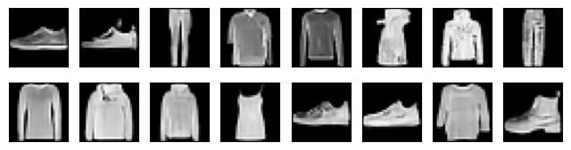
@nnx.jit
def euler50(net, noise):
    pred = d2l.make_pred(net, path, 'velocity')
    return d2l.ode_sample(pred, noise, path.sigma_bars(50))

def sample(net, shape, n=5000):
    """n samples by 50 Euler steps from fixed noise, 1,000 at a time."""
    noise = jax.random.normal(jax.random.key(0), (n, *shape))
    return d2l.batched(lambda x: euler50(net, x), noise)

def decode(z):
    return d2l.batched(lambda z_k: decoder(ae, z_k / scale), z)

latent_shape, image_shape = (7, 7, 4), (28, 28, 1)
x_pixel = sample(unet_pixel, image_shape)
x_latent = decode(sample(unet_latent, latent_shape))
fd_pixel, fd_latent = fd(x_pixel), fd(x_latent)
print(f'FD: pixel U-Net {fd_pixel:.2f}, latent U-Net {fd_latent:.2f}')
d2l.show_gray(jnp.concatenate([x_pixel[:8], x_latent[:8]]), 2, 8);
FD: pixel U-Net 1.58, latent U-Net 2.27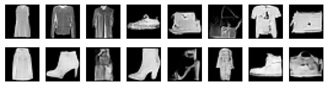
Both rows show recognizable garments. The latent model scores an FD of about 2 (2.0 to 2.4), the pixel model 1.5 to 1.6.
What did the latent model save? train_step_gflops counts the floating-point operations of one training step, forward and backward on 128 inputs, in billions (GFLOP).
def train_step_gflops(net, loss_fn, shape, batch_size=128):
    """GFLOP of one training step, forward and backward, on a batch of zeros
    of the given shape."""
    from torch.utils.flop_counter import FlopCounterMode  # not in the preamble
    x = torch.zeros(batch_size, *shape, device=next(net.parameters()).device)
    with FlopCounterMode(display=False) as counter:
        loss_fn(net, x).backward()
    return counter.get_total_flops() / 1e9
def train_step_gflops(net, loss_fn, shape, batch_size=128):
"""GFLOP of one training step, forward and backward, on a batch of zeros
of the given shape: XLA's estimate for the step lowered for the CPU (for
a GPU it leaves out the convolutions)."""
graphdef, params, rest = nnx.split(net, nnx.Param, ...)
grad = jax.grad(lambda p, r, x, key: loss_fn(nnx.merge(graphdef, p, r),
x, key))
args = jax.device_put((params, rest, jnp.zeros((batch_size, *shape)),
jax.random.key(0)), jax.devices('cpu')[0])
return jax.jit(grad).lower(*args).cost_analysis()['flops'] / 1e9gflops_latent = d2l.train_step_gflops(
d2l.UNet(ch=64, in_channels=4, out_channels=4).to(dev), loss_fn,
latent_shape)
gflops_pixel = d2l.train_step_gflops(d2l.UNet(ch=64).to(dev), loss_fn,
image_shape)
print(f'GFLOP per training step: latent U-Net {gflops_latent:.0f}, '
f'pixel U-Net {gflops_pixel:.0f}')GFLOP per training step: latent U-Net 15, pixel U-Net 203gflops_latent = d2l.train_step_gflops(
d2l.UNet(ch=64, in_channels=4, out_channels=4, rngs=nnx.Rngs(0)), loss_fn,
latent_shape)
gflops_pixel = d2l.train_step_gflops(d2l.UNet(ch=64, rngs=nnx.Rngs(0)),
loss_fn, image_shape)
print(f'GFLOP per training step: latent U-Net {gflops_latent:.0f}, '
f'pixel U-Net {gflops_pixel:.0f}')GFLOP per training step: latent U-Net 11, pixel U-Net 192The latent U-Net needs about a dozen GFLOP per step, the pixel U-Net about 200. Every evaluation of the latent network, in training and at each sampling step, costs less than a tenth of the arithmetic.
17.6.2.2 Reading the Result
At equal updates the latent model’s FD is about 1.4 to 1.5 times the pixel model’s. It cannot fall below the reconstruction FD of 0.6 to 0.8, and it sits well above it. The gap combines the latent model’s own error with the decoder’s response to latents that no training image produced.
At \(28 \times 28\) the trade is not attractive: the pixel model is cheap anyway, and the autoencoder needs a training run of its own. At \(512 \times 512\) the factor of 48 applies to every convolution, and for a transformer with \(2 \times 2\) patches the number of tokens falls from 65,536 to 1,024, so attention, whose cost grows with their square, becomes 4,096 times cheaper. This is why most large text-to-image systems since 2022 diffuse latents, and why their autoencoder limits their quality, a limit we measure once we have a second network to try.
17.6.3 The Transformer Backbone
The U-Net builds in the assumptions of a convolutional network: nearby pixels matter most, and the same features can appear anywhere. The vision transformer of Section 11.5 makes fewer of them, and on image classification it trails convolutional networks at small budgets and overtakes them at large ones. Peebles and Xie (2023) asked whether the same holds for diffusion.
17.6.3.1 Patches and Tokens
The DiT reads its input as the vision transformer does. It cuts the image into \(p \times p\) patches, maps each to a vector of width \(d\) by a linear map (a convolution with kernel size and stride \(p\)), adds a learned position embedding, and passes the tokens through pre-norm transformer blocks (Section 11.1). With \(p = 4\) a \(28 \times 28\) image becomes 49 tokens of 16 pixels each; on our latents with \(p = 1\), each of the 49 grid positions is a token of four numbers.
The output differs from a classifier’s. A denoiser returns a prediction of the shape of its input, so the DiT maps every token by a final linear layer to the values of its patch and reassembles the patches. Each token predicts the velocity of its own patch, informed through attention by all the others. With one token per pixel the image would have 16 times as many tokens, and attention would cost 256 times as much.
17.6.3.2 Adaptive Layer Norm
The transformer also needs the time \(t\), and possibly a label. Peebles and Xie (2023) compared ways to condition it, among them appending the condition as extra tokens, and found that the cheapest worked best: the condition sets the normalization.
A layer norm standardizes each token and applies a learned scale and shift. In adaptive layer norm a linear map computes the scale \(\mathbf{a}\) and the shift \(\mathbf{b}\) from the condition \(\mathbf{c}\), the sum of a time embedding and a label embedding, and the condition also sets a gate \(\mathbf{g}\) on each sublayer’s output. One block computes
\[ \begin{aligned} \mathbf{X} &\leftarrow \mathbf{X} + \mathbf{g}_1 \odot \mathrm{Attention}\big(\mathrm{LN}(\mathbf{X}) \odot (1 + \mathbf{a}_1) + \mathbf{b}_1\big),\\ \mathbf{X} &\leftarrow \mathbf{X} + \mathbf{g}_2 \odot \mathrm{MLP}\big(\mathrm{LN}(\mathbf{X}) \odot (1 + \mathbf{a}_2) + \mathbf{b}_2\big), \end{aligned} \]
where \(\mathrm{LN}\) has no scale or shift of its own and the six vectors are one linear function of \(\mathbf{c}\), shared by all tokens of an image. One small matrix product per image thus turns each feature of each sublayer up or down.
The linear map starts at zero, hence the name adaLN-Zero. All gates are then zero, every block computes the identity, and the final layer, also zero, outputs zero. Training starts from a network that predicts zero velocity everywhere, and each block comes into play as its gates grow (Figure 17.6.2).
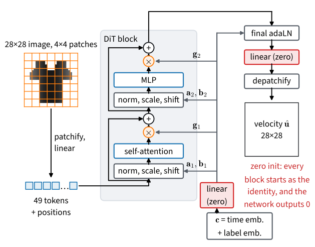
DiTBlock builds the block on the ViTBlock of Section 11.5, with ada as the linear map.
class DiTBlock(d2l.ViTBlock):
    """ViTBlock with adaLN-Zero: the condition c sets a shift, a scale and a
    gate for each sublayer; the gates start at zero."""
    def __init__(self, num_hiddens, mlp_num_hiddens, num_heads):
        super().__init__(num_hiddens, mlp_num_hiddens, num_heads, dropout=0.0,
                         use_bias=True)
        ln = lambda: nn.LayerNorm(num_hiddens, elementwise_affine=False,
                                  eps=1e-6)
        self.norm1, self.norm2 = ln(), ln()
        self.ada = nn.Sequential(nn.SiLU(),
                                 nn.Linear(num_hiddens, 6 * num_hiddens))
        nn.init.zeros_(self.ada[1].weight), nn.init.zeros_(self.ada[1].bias)

    def forward(self, X, c):
        shift1, scale1, gate1, shift2, scale2, gate2 = (
            self.ada(c)[:, None].chunk(6, dim=-1))
        X_mod = self.norm1(X) * (1 + scale1) + shift1
        X = X + gate1 * self.attention(X_mod, X_mod, X_mod)
        return X + gate2 * self.ffn(self.norm2(X) * (1 + scale2) + shift2)
class DiTBlock(d2l.ViTBlock):
"""ViTBlock with adaLN-Zero: the condition c sets a shift, a scale and a
gate for each sublayer; the gates start at zero."""
def __init__(self, num_hiddens, mlp_num_hiddens, num_heads, *, rngs):
super().__init__(num_hiddens, mlp_num_hiddens, num_heads, 0.0,
use_bias=True, rngs=rngs)
ln = lambda: nnx.LayerNorm(num_hiddens, epsilon=1e-6, use_scale=False,
use_bias=False, rngs=rngs)
self.norm1, self.norm2 = ln(), ln()
zeros = nnx.initializers.zeros
self.ada = nnx.Linear(num_hiddens, 6 * num_hiddens, kernel_init=zeros,
bias_init=zeros, rngs=rngs)
def __call__(self, X, c):
shift1, scale1, gate1, shift2, scale2, gate2 = jnp.split(
self.ada(nnx.silu(c))[:, None], 6, axis=-1)
X_mod = self.norm1(X) * (1 + scale1) + shift1
X = X + gate1 * self.attention(X_mod, X_mod, X_mod)
return X + gate2 * self.ffn(self.norm2(X) * (1 + scale2) + shift2)DiT adds the patch embedding, the learned positions, the time and label embeddings, and the final adaptive layer norm and linear layer.
class DiT(nn.Module):
    """Diffusion transformer conditioned on a time t in [0, 1] and, with
    num_classes, on a label y; label num_classes means no label."""
    def __init__(self, img_size=28, patch_size=4, num_channels=1, width=256,
                 depth=6, num_heads=4, num_classes=None):
        super().__init__()
        self.width, self.num_classes = width, num_classes
        self.p, self.g = patch_size, img_size // patch_size
        self.patch = d2l.PatchEmbedding(img_size, patch_size, width,
                                        num_channels)
        self.pos = nn.Parameter(0.02 * torch.randn(1, self.g ** 2, width))
        self.time_mlp = d2l.make_mlp([width] * 3, nn.SiLU())
        self.label_emb = (nn.Embedding(num_classes + 1, width)
                          if num_classes else None)
        self.blks = nn.ModuleList([DiTBlock(width, 4 * width, num_heads)
                                   for _ in range(depth)])
        self.ln = nn.LayerNorm(width, elementwise_affine=False, eps=1e-6)
        self.ada = nn.Sequential(nn.SiLU(), nn.Linear(width, 2 * width))
        self.out = nn.Linear(width, patch_size ** 2 * num_channels)
        for m in (self.ada[1], self.out):
            nn.init.zeros_(m.weight), nn.init.zeros_(m.bias)

    def forward(self, x, t, y=None):
        c = self.time_mlp(d2l.time_embedding(t, self.width))
        if y is not None:
            c = c + self.label_emb(y)
        X = self.patch(x) + self.pos
        for blk in self.blks:
            X = blk(X, c)
        shift, scale = self.ada(c)[:, None].chunk(2, dim=-1)
        X = self.out(self.ln(X) * (1 + scale) + shift)  # (n, g*g, p*p*c)
        n, g, p = len(x), self.g, self.p  # tokens back to pixels
        X = X.reshape(n, g, g, p, p, -1).permute(0, 5, 1, 3, 2, 4)
        return X.reshape(n, -1, g * p, g * p)
class DiT(nnx.Module):
"""Diffusion transformer (NHWC) conditioned on a time t in [0, 1] and,
with num_classes, on a label y; label num_classes means no label."""
def __init__(self, img_size=28, patch_size=4, num_channels=1, width=256,
depth=6, num_heads=4, num_classes=None, *, rngs):
self.width, self.num_classes = width, num_classes
self.p, self.g = patch_size, img_size // patch_size
self.patch = d2l.PatchEmbedding(img_size, patch_size, width,
num_channels, rngs=rngs)
self.pos = nnx.Param(
0.02 * rngs.params.normal((1, self.g ** 2, width)))
self.time_mlp = d2l.make_mlp([width] * 3, nnx.silu, rngs=rngs)
init = nnx.initializers.normal(1.0) # N(0, 1), as in PyTorch
self.label_emb = (nnx.Embed(num_classes + 1, width, rngs=rngs,
embedding_init=init)
if num_classes else None)
self.blks = nnx.List([DiTBlock(width, 4 * width, num_heads, rngs=rngs)
for _ in range(depth)])
self.ln = nnx.LayerNorm(width, epsilon=1e-6, use_scale=False,
use_bias=False, rngs=rngs)
zeros = nnx.initializers.zeros
self.ada = nnx.Linear(width, 2 * width, kernel_init=zeros,
bias_init=zeros, rngs=rngs)
self.out = nnx.Linear(width, patch_size ** 2 * num_channels,
kernel_init=zeros, bias_init=zeros, rngs=rngs)
def __call__(self, x, t, y=None):
c = self.time_mlp(d2l.time_embedding(t, self.width))
if y is not None:
c = c + self.label_emb(y)
X = self.patch(x) + self.pos[...]
for blk in self.blks:
X = blk(X, c)
shift, scale = jnp.split(self.ada(nnx.silu(c))[:, None], 2, axis=-1)
X = self.out(self.ln(X) * (1 + scale) + shift) # (n, g*g, p*p*c)
n, g, p = x.shape[0], self.g, self.p # tokens back to pixels
X = X.reshape(n, g, g, p, p, -1).transpose(0, 1, 3, 2, 4, 5)
return X.reshape(n, g * p, g * p, -1)We build a DiT of width 256 and depth 6 with four heads, and pass eight images and times through it.
dit = d2l.DiT().to(dev)       # width 256, depth 6, 4 heads, 4 x 4 patches
x, t = X[:8], torch.rand(8, device=dev)
with torch.no_grad():
    tokens, out = dit.patch(x), dit(x, t)
print('images', tuple(x.shape), '-> tokens', tuple(tokens.shape),
      '-> output', tuple(out.shape))
print(f'parameters: DiT {d2l.num_params(dit) / 1e6:.2f}M, '
      f'U-Net {d2l.num_params(d2l.UNet(ch=64)) / 1e6:.2f}M')
print('output at initialization all zero:', bool((out == 0).all()))
images (8, 1, 28, 28) -> tokens (8, 49, 256) -> output (8, 1, 28, 28)
parameters: DiT 7.39M, U-Net 1.20M
output at initialization all zero: Truedit = d2l.DiT(rngs=nnx.Rngs(0)) # width 256, depth 6, 4 heads, 4 x 4 patches
x, t = X[:8], jax.random.uniform(jax.random.key(5), (8,))
tokens, out = dit.patch(x), dit(x, t)
print('images', x.shape, '-> tokens', tokens.shape, '-> output', out.shape)
print(f'parameters: DiT {d2l.num_params(dit) / 1e6:.2f}M, U-Net '
f'{d2l.num_params(d2l.UNet(ch=64, rngs=nnx.Rngs(0))) / 1e6:.2f}M')
print('output at initialization all zero:', bool((out == 0).all()))images (8, 28, 28, 1) -> tokens (8, 49, 256) -> output (8, 28, 28, 1)
parameters: DiT 7.39M, U-Net 1.20M
output at initialization all zero: TrueThe DiT has 7.39 million parameters, six times as many as the U-Net, and its untrained output is exactly zero.
17.6.3.3 Scaling with Compute
Is the transformer better than the U-Net? At one size the question has no general answer. Peebles and Xie (2023) trained DiTs of four sizes with three patch sizes each. At a fixed number of training steps, FID fell steadily as the network’s arithmetic per forward pass grew, whether it came from a larger network or from smaller patches, and their largest model, trained for seven million steps, set a new best FID on class-conditional ImageNet at \(256 \times 256\).
We repeat the measurement at our scale. Three DiTs grow in width and depth together, with 64 dimensions per head as in the paper: DiT-S (width 128, depth 4, two heads), DiT-M (the model above) and DiT-L (width 384, depth 8, six heads). Each is trained on pixels with the U-Net’s loss and recipe for the same 20,000 updates, and we measure its size by the FLOPs per training step.
sizes = {'DiT-S': dict(width=128, depth=4, num_heads=2),
         'DiT-M': dict(width=256, depth=6, num_heads=4),
         'DiT-L': dict(width=384, depth=8, num_heads=6)}
runs = {}
for seed, (name, size) in enumerate(sizes.items(), start=5):
    gflops = d2l.train_step_gflops(d2l.DiT(**size).to(dev), loss_fn,
                                   image_shape)
    torch.manual_seed(seed)
    net = d2l.DiT(**size).to(dev)
    _, ema, _ = d2l.train_regression(net, loss_fn, batch_fn, 20_000)
    imgs = sample(ema, image_shape)
    runs[name] = dict(params=d2l.num_params(net), gflops=gflops, fd=fd(imgs),
                      imgs=imgs[:8])
runs['U-Net'] = dict(params=d2l.num_params(d2l.UNet(ch=64)),
                     gflops=gflops_pixel, fd=fd_pixel, imgs=x_pixel[:8])
for name, run in runs.items():
    print(f'{name:6} {run["params"] / 1e6:5.2f}M parameters '
          f'{run["gflops"]:4.0f} GFLOP per step   FD {run["fd"]:.2f}')
DiT-S 1.26M parameters 32 GFLOP per step FD 5.27
DiT-M 7.39M parameters 185 GFLOP per step FD 1.73
DiT-L 21.90M parameters 550 GFLOP per step FD 1.36
U-Net 1.20M parameters 203 GFLOP per step FD 1.50sizes = {'DiT-S': dict(width=128, depth=4, num_heads=2),
'DiT-M': dict(width=256, depth=6, num_heads=4),
'DiT-L': dict(width=384, depth=8, num_heads=6)}
runs = {}
for seed, (name, size) in enumerate(sizes.items(), start=5):
gflops = d2l.train_step_gflops(d2l.DiT(**size, rngs=nnx.Rngs(0)),
loss_fn, image_shape)
net = d2l.DiT(**size, rngs=nnx.Rngs(seed))
_, ema, _ = d2l.train_regression(net, loss_fn, batch_fn, 20_000,
jax.random.key(seed))
imgs = sample(ema, image_shape)
runs[name] = dict(params=d2l.num_params(net), gflops=gflops, fd=fd(imgs),
imgs=imgs[:8])
runs['U-Net'] = dict(params=d2l.num_params(d2l.UNet(ch=64, rngs=nnx.Rngs(0))),
gflops=gflops_pixel, fd=fd_pixel, imgs=x_pixel[:8])
for name, run in runs.items():
print(f'{name:6} {run["params"] / 1e6:5.2f}M parameters '
f'{run["gflops"]:4.0f} GFLOP per step FD {run["fd"]:.2f}')DiT-S 1.26M parameters 33 GFLOP per step FD 4.96
DiT-M 7.39M parameters 190 GFLOP per step FD 1.61
DiT-L 21.90M parameters 559 GFLOP per step FD 1.19
U-Net 1.20M parameters 192 GFLOP per step FD 1.58We plot FD against FLOPs per step on logarithmic axes.
dits = [runs[name] for name in sizes]
d2l.plot([[run['gflops'] for run in dits], [runs['U-Net']['gflops']]],
         [[run['fd'] for run in dits], [runs['U-Net']['fd']]],
         'GFLOP per training step', 'FD (5,000 samples)',
         legend=['DiT-S, M, L', 'U-Net'], xscale='log', yscale='log',
         fmts=('o-', 'rD'))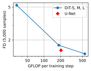
dits = [runs[name] for name in sizes]
d2l.plot([[run['gflops'] for run in dits], [runs['U-Net']['gflops']]],
         [[run['fd'] for run in dits], [runs['U-Net']['fd']]],
         'GFLOP per training step', 'FD (5,000 samples)',
         legend=['DiT-S, M, L', 'U-Net'], xscale='log', yscale='log',
         fmts=('o-', 'rD'))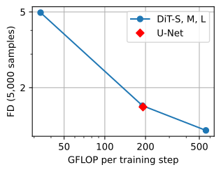
FD falls with every step up in size: about 5 for DiT-S at about 30 GFLOP per step, 1.5 to 1.7 for DiT-M at about 190, and 1.2 to 1.5 for DiT-L at about 550. The first sixfold increase in compute divides the FD by about three; the next threefold increase gains less. The U-Net, at 1.5 to 1.6 and about 200 GFLOP, matches or slightly beats DiT-M, which spends the same arithmetic with six times the parameters, and DiT-L beats it.
The rows below show the first eight samples of DiT-S, DiT-M and DiT-L, drawn from the same noise.
d2l.show_gray(torch.cat([run['imgs'] for run in dits]), 3, 8);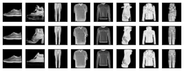
d2l.show_gray(jnp.concatenate([run['imgs'] for run in dits]), 3, 8);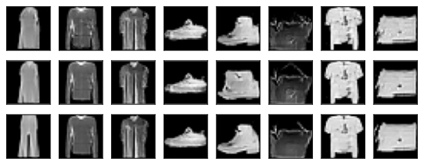
The three models mostly draw the same garment from the same noise, since each integrates an ODE that sends a noise image to one image. DiT-S draws it with blotches and broken outlines, and each larger model sharpens it.
At equal parameters the U-Net wins by a wide margin: DiT-S has as many parameters and three times the FD. The convolutional assumptions are worth much on a small budget, and the transformer overtakes the U-Net only by growing. What makes it the backbone at scale is that it keeps improving as it grows, by a recipe as simple as making it wider and deeper. Its arithmetic runs as large matrix products, and the methods that train language models at scale carry over. Our horizontal axis is compute per update. Whether a large model trained for fewer updates beats a small one trained for more, at equal total compute, is a separate question (11).
Does the transformer help in the latent space too? We train DiT-M on the latents with patches of size 1, so that it sees 49 tokens and spends the same arithmetic per step as in pixel space.
gflops = d2l.train_step_gflops(
    d2l.DiT(img_size=7, patch_size=1, num_channels=4, **sizes['DiT-M']).to(dev),
    loss_fn, latent_shape)
torch.manual_seed(8)
net = d2l.DiT(img_size=7, patch_size=1, num_channels=4,
              **sizes['DiT-M']).to(dev)
_, dit_latent, _ = d2l.train_regression(net, loss_fn, latent_batch_fn, 20_000)
print(f'latent DiT-M, {gflops:.0f} GFLOP per step: FD '
      f'{fd(decode(sample(dit_latent, latent_shape))):.2f}; latent U-Net '
      f'{fd_latent:.2f}; reconstructions {fd_rec:.2f}')
latent DiT-M, 185 GFLOP per step: FD 1.93; latent U-Net 2.07; reconstructions 0.65gflops = d2l.train_step_gflops(
d2l.DiT(img_size=7, patch_size=1, num_channels=4, **sizes['DiT-M'],
rngs=nnx.Rngs(0)), loss_fn, latent_shape)
net = d2l.DiT(img_size=7, patch_size=1, num_channels=4, **sizes['DiT-M'],
rngs=nnx.Rngs(8))
_, dit_latent, _ = d2l.train_regression(net, loss_fn, latent_batch_fn, 20_000,
jax.random.key(8))
print(f'latent DiT-M, {gflops:.0f} GFLOP per step: FD '
f'{fd(decode(sample(dit_latent, latent_shape))):.2f}; latent U-Net '
f'{fd_latent:.2f}; reconstructions {fd_rec:.2f}')latent DiT-M, 190 GFLOP per step: FD 2.15; latent U-Net 2.27; reconstructions 0.78The latent DiT-M scores an FD of about 2 (1.8 to 2.3), at or a little below the latent U-Net’s, although in pixel space it reached 1.5 to 1.7. In the latent space the backbone matters little: both land at about three times the reconstruction FD. Both backbones, a dozen and two hundred GFLOP per step, land at about the same FD, so the limit lies with the autoencoder, its reconstructions and its decoder’s response to slightly wrong latents (10). At our scale the best pixel model therefore beats every latent one. At \(512 \times 512\) the saving decides, but the limit remains, which is why the design of image autoencoders, often called tokenizers, has become a field of its own.
17.6.4 Conditioning on Text and Beyond
17.6.4.1 Cross-Attention and Joint Attention
A caption enters the model as a sequence of vectors. A frozen text encoder, such as the text half of CLIP (Radford et al. 2021) or the encoder of T5 (Raffel et al. 2020), turns the caption into one vector per token, and the denoiser attends to them. In the U-Net of Rombach et al. (2022), cross-attention layers let the image positions query the caption vectors as keys and values. Esser et al. (2024) instead concatenate image and caption tokens into one sequence and attend over both, with separate weights for each kind of token; this multimodal DiT (MMDiT) is the backbone of Stable Diffusion 3. Training needs one ingredient this chapter already has. The caption is dropped with a small probability, as the label was in Section 17.3.4.2, so the empty caption plays the null label \(\varnothing\), and classifier-free guidance combines the two predictions as before, \(\tilde{\mathbf{u}} = \mathbf{u}_{\boldsymbol\theta}(\mathbf{x}, t, \varnothing) + \gamma\,(\mathbf{u}_{\boldsymbol\theta}(\mathbf{x}, t, c) - \mathbf{u}_{\boldsymbol\theta}(\mathbf{x}, t, \varnothing))\), with \(c\) now the caption. Esser et al. also draw the training times from the logit-normal distribution of Section 17.5.
17.6.4.2 Video
A video is a stack of frames, and the recipe applies once the stack is compressed. A three-dimensional autoencoder compresses space and time together, typically eightfold along each side of a frame and fourfold or more in time, and the transformer attends over patches that span a few frames each. Ho et al. (2022) trained the first video diffusion models on pixels, Blattmann et al. (2023) adapted a latent image model to video, and Polyak et al. (2024) trained a transformer of 30 billion parameters on video latents. The number of tokens sets the cost: a few seconds of video make tens of thousands of tokens, and attention over all of them dominates training.
17.6.5 Summary
Diffusion does not need to run on pixels. An autoencoder with a small KL term compresses each image into a latent of known scale, the regression of the previous sections runs on the latents unchanged, and the decoder turns sampled latents back into images. Each network evaluation then costs a fraction of a pixel model’s, while the reconstructions of the autoencoder limit the quality of the samples. The diffusion transformer reads latents or pixels as patch tokens and lets the time set a scale, a shift and a gate in every block, starting from the identity. At equal updates its FD fell steadily with its compute per step, and its largest version beat the U-Net. A caption enters as tokens through attention, and video as tokens over space and time. However cheap each evaluation is, fifty evaluations per sample remain fifty; the next section asks how to get by with one or two.
17.6.6 Exercises
- The scale of the latents. The linear path mixes the data with noise of unit variance.
- Suppose each latent value has standard deviation \(\varsigma\) instead of one. Show that its signal-to-noise ratio at time \(t\) is \(\varsigma^2 (1 - t)^2 / t^2\), so that the log-SNR is shifted by \(\log \varsigma^2\) at every time.
- At which time does a latent with \(\varsigma = 5\) have the signal-to-noise ratio that a latent with \(\varsigma = 1\) has at \(t = \tfrac12\)? What fraction of uniformly drawn training times then falls where the signal still dominates the noise?
- [code] Train the latent U-Net on latents multiplied by \(5c\) instead of \(c\), and compare the decoded FD. Relate the result to the shift of the schedule with resolution in Section 17.5.3.2.
- Tokens at high resolution. The autoencoder of Stable Diffusion maps a \(512 \times 512 \times 3\) image to \(64 \times 64 \times 4\).
- How many tokens does a DiT see with patches of size 2 on the latent, and with patches of size 16 on the pixels? How many numbers does each token carry in the two cases?
- A DiT block of width \(d\) has about \(12 d^2\) weights, and a training step costs about six FLOPs per weight and token, plus the attention. Estimate the FLOPs of one training step on a batch of 256 for a DiT of width 1,152 and depth 28 on the latents with patch 2. How large is the attention part?
- With patch 16 on the pixels the DiT sees as many tokens as with patch 2 on the latents, at almost the same cost. What does the autoencoder provide that a linear patch embedding does not?
- [code] Why start at zero. Replace the zero initialization of the
adalayers ind2l.DiTBlockandd2l.DiTby the framework’s default initialization.- Print the size of the output of the untrained network for both initializations.
- Train both DiT-M models for 2,000 updates and plot their losses. Explain the difference through the identity at initialization.
- [code] Patch size. ● Train DiT-M with patches of size 2 on the pixels for 20,000 updates.
- How many tokens does it see, and how many FLOPs per step does
train_step_gflopscount? Is the increase over patch 4 what the cost of attention predicts? - Where does its FD fall on the curve of DiT-S, DiT-M and DiT-L? Does FD depend on the compute per step alone, whatever produces it?
- How many tokens does it see, and how many FLOPs per step does
- [code] Large patches and the clean-image target. ● Train
DiTon pixels withpatch_size=7, so that each of its 16 tokens carries 49 pixel values, at width 32 with one head and at width 256, for 10,000 updates each. Give each width two output parameterizations under the same velocity loss: the network outputs the velocity, or it outputs \(\hat{\mathbf{x}}_0\) and the velocity is formed as \((\mathbf{x}_t - \hat{\mathbf{x}}_0)/t\), with \(t\) clamped below at \(0.05\).- Report the FD of the four models in a \(2 \times 2\) table.
- Does the clean-image output help at width 32, where a token carries more values than the network has channels, and does the gap close at width 256?
- Explain the result with the argument of Section 17.5: an image lies near a set of much lower dimension than its pixel count, while the noise fills every dimension. Compare with the finding of Li and He (2026) .
- [code] Width of the bottleneck. Train autoencoders with 2, 4 and 8 latent channels.
- Report the reconstruction FD of each and the decoded FD of a latent U-Net trained on each.
- Which of the two numbers moves more, and does the gap between them close as the latent grows? What does this suggest about the four channels of Stable Diffusion’s autoencoder, and the 16 or more of later ones?
- [code] The KL weight. Train the autoencoder with \(\beta \in \{0, 10^{-3}, 10^{-2}\}\).
- For each, print the latent standard deviation, the encoder’s standard deviation, the excess kurtosis and the reconstruction FD.
- Train a latent U-Net on each and report the decoded FD. Which \(\beta\) gives the best samples, and why is it not the one whose latents are closest to normal?
- With \(\beta = 0\) nothing ties the scale of the latents to one. Why does the scale factor \(c\) still make the latents usable?
- Captions and guidance. A text-to-image model is trained with the caption replaced by the empty caption 10% of the time.
- What distribution does the network learn to sample when it is given the empty caption? What would guidance do if the caption were never dropped?
- Guidance needs two predictions per step. Compare the cost of two forward passes with that of one pass on a doubled batch, for a DiT with cross-attention and for an MMDiT, where the empty caption also changes the length of the joint sequence.
- Cross-attention as a lookup. Image tokens \(\mathbf{Y} \in \mathbb{R}^{m \times d}\) query caption tokens \(\mathbf{X} \in \mathbb{R}^{n \times d}\), with queries \(\mathbf{Y}\mathbf{W}_q\), keys \(\mathbf{X}\mathbf{W}_k\) and values \(\mathbf{X}\mathbf{W}_v\).
- Show that each image position receives a convex combination of the caption’s value vectors. With an empty caption of one token, show that every position receives the same vector, so that the unconditional prediction of guidance sees cross-attention as a learned constant shift.
- Suppose that the values were computed from the image instead, \(\mathbf{V} = \mathbf{Y}\mathbf{W}_v\). What goes wrong with the shapes when \(m \neq n\), and what would such a layer compute when \(m = n\)?
- In cross-attention the caption’s keys and values do not depend on \(\mathbf{x}_t\); in an MMDiT the caption tokens are updated by the image tokens in every block. For a caption of 77 tokens, 1,024 image tokens and 50 steps with guidance, which caption-side computations can a cross-attention model do once per sample, and what fraction of an MMDiT’s token computations belongs to the caption?
- [code] Scaling in the latent space. ● Train DiT-S and DiT-L on the latents, as DiT-M was trained above.
- Add the three latent models to the plot of FD against FLOPs per step, with the reconstruction FD as a horizontal line. Does the latent curve keep falling with size?
- Explain the shape of the latent curve through the decoder. What would you change to move it down?
- [code] Compute per step and compute in total. ● Change the training of the three pixel DiTs so that each is scored after 5,000, 10,000 and 20,000 updates.
- Plot FD against total training compute, the FLOPs per step times the number of updates, with one curve per model.
- At equal total compute, does the larger model reach the lower FD? Compare with the plot of FD against total training compute in the paper of Peebles and Xie, and say what longer runs could change.
- At 10,000 updates, does DiT-L still beat the U-Net?
- [extended] Latent diffusion for sprites. ●● Adapt this section’s autoencoder to the \(64 \times 64\) color sprites of Section 16.5, which gives a \(16 \times 16 \times 4\) latent, and train a latent U-Net on it. Score the samples with the
d2l.FeatureCNNof Section 16.5 and compare them with the GANs trained there. Which of the two methods needs more compute for the same FD?