%matplotlib inline
from d2l import torch as d2l
import time
import torch
from torch import nn

# Let fp32 matmuls use tf32 tensor cores; off by default, and every timing
# in this chapter is misleading without it (see :numref:`sec_memory_precision`).
torch.set_float32_matmul_precision('high')13.1 The Performance Model
Run one matrix multiplication at two sizes on the same GPU with correct synchronization, and the hardware can deliver very different fractions of its advertised speed. A small multiplication may achieve one percent of peak throughput, whereas a large one can approach the specification. This section explains the difference and develops a method for diagnosing it.
The method has four steps: measure what the program does; classify which of three resources binds it — arithmetic, memory bandwidth, or per-operation overhead; fix the binding constraint with the matching technique; then re-measure, because the fix moves the bottleneck somewhere else. Every later section of this chapter slots into this loop. Section 13.2 explains where the machine’s two headline numbers come from; Section 13.3 targets the bandwidth and overhead regimes; Section 13.4 buys back memory and trades precision for speed; Section 13.5 and Section 13.6 add devices; Section 13.7 runs the whole loop on a real Transformer.
The analysis uses two quantities. The first is arithmetic intensity: how many floating-point operations a computation performs per byte it moves to and from memory. Compared against a single machine-dependent threshold, intensity predicts which regime an operation lands in — before you run anything. The second is that timing a GPU is easy to get wrong: the frameworks dispatch work asynchronously, so a naive timer measures how fast Python can enqueue work, not how fast the GPU can do it. We build the measurement discipline first, package it into a small tool used throughout the chapter, and then use it to map our own GPU.
Prerequisites: tensors and GPU placement from Section 5.7; the training loop of Section 2.4. No new modeling ideas appear here — this section is about the machine.
%matplotlib inline
from d2l import jax as d2l
import jax
from jax import numpy as jnp
import numpy as np
import time
13.1.1 Counting: FLOPs, Bytes, and Arithmetic Intensity
Every tensor operation makes two demands on the hardware: it asks for arithmetic — some number of floating-point operations (FLOPs) — and it asks for bytes — its inputs must be fetched from memory and its outputs written back. A GPU has a separate budget for each. Our build machine’s RTX 4090 can execute about \(165 \times 10^{12}\) FLOP/s on bf16 tensor cores, and can move about \(1.0 \times 10^{12}\) bytes/s between its compute units and its memory. Which budget runs out first depends on the ratio the operation asks for:
\[ \textrm{arithmetic intensity} \;=\; \frac{\textrm{FLOPs performed}}{\textrm{bytes moved}}. \]
Consider the workhorse: a matrix multiplication \(\mathbf{X}\mathbf{W}\) with \(\mathbf{X} \in \mathbb{R}^{B \times D}\) and \(\mathbf{W} \in \mathbb{R}^{D \times F}\). It performs \(2BDF\) FLOPs (one multiply and one add per term), while touching \(BD + DF + BF\) numbers. With \(b\) bytes per element, the intensity is
\[ \frac{2BDF}{b\,(BD + DF + BF)} \;=\; \frac{2}{b}\left(\frac{1}{F} + \frac{1}{B} + \frac{1}{D}\right)^{-1} \;\approx\; \frac{2B}{b} \quad \textrm{for } B \ll D, F. \tag{13.1.1}\]
The approximation has a direct scaling consequence: for a skinny batch pushed through a wide layer, intensity grows linearly with the batch size, because each weight fetched from memory is reused across every row of the batch. A batch of one reuses nothing — each weight is fetched, used once, and discarded. This single observation will explain phenomena from “why big batches are fast” to why generating from a language model one token at a time is memory-bound (Section 13.2).
An elementwise operation sits at the other extreme: \(y_i = x_i + 1\) performs one FLOP per element while moving \(2b\) bytes (read \(x_i\), write \(y_i\)), an intensity of \(1/(2b)\) — a fraction of a FLOP per byte, no matter how large the tensor.
The roofline model (Williams et al. 2009) converts arithmetic intensity into an upper bound. An operation with intensity \(I\) running on a machine with peak compute \(P\) (FLOP/s) and memory bandwidth \(\beta\) (bytes/s) can attain at most
\[ \textrm{performance} \;\leq\; \min(P,\; I \cdot \beta). \tag{13.1.2}\]
Plotted on log–log axes (Figure 13.1.1), the bandwidth bound rises with intensity until it meets the flat compute roof. The intersection is the ridge point \(I^* = P/\beta\): operations with intensity below \(I^*\) are bandwidth-bound — the memory system cannot feed the arithmetic units fast enough. Additional arithmetic does not increase elapsed time while memory traffic remains limiting; operations above it are compute-bound — the arithmetic units are saturated, and moving fewer bytes would not help.
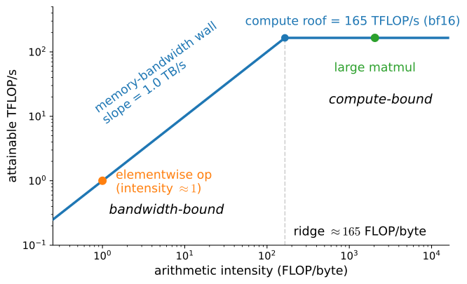
Let’s compute the ridge point for the card this book is built on. Peak tensor-core throughput is not exposed programmatically, so we take it from the specification sheet; the device query tells us what we are running on.
prop = torch.cuda.get_device_properties(0)
peak_tflops = 165.0   # RTX 4090 dense bf16 tensor-core spec
bandwidth_tbs = 1.008  # GDDR6X spec
print(f'{prop.name}, {prop.total_memory / 1e9:.0f} GB')
print(f'ridge point = {peak_tflops / bandwidth_tbs:.0f} FLOP/byte')
NVIDIA GeForce RTX 4090, 25 GB
ridge point = 164 FLOP/bytedevice = jax.devices()[0]
peak_tflops = 165.0 # RTX 4090 dense bf16 tensor-core spec
bandwidth_tbs = 1.008 # GDDR6X spec
print(f'{device.device_kind}')
print(f'ridge point = {peak_tflops / bandwidth_tbs:.0f} FLOP/byte')NVIDIA GeForce RTX 4090
ridge point = 164 FLOP/byteA ridge point of about 165 FLOP/byte means the machine wants about 165 arithmetic operations for every byte it fetches, just to break even — and our consumer card is on the low side; across modern accelerators the ridge sits anywhere from a hundred to several hundred FLOP/byte. Very little of what a neural network does naturally reaches that ratio — which is why the rest of this chapter is mostly about bytes, not FLOPs. For the square matmul above (\(B = D = F = n\), bf16), intensity is \(n/3\): in principle, sizes beyond \(n \approx 500\) stop being bandwidth-limited. The measured sweep below shows that occupancy and launch overhead also determine the crossover. Section 13.2 explains where \(P\) and \(\beta\) come from physically, and why their ratio has climbed, over the long run, from one hardware generation to the next.
13.1.2 Correct GPU Timing
Mapping a GPU against the roofline requires synchronized timing. Timing only the asynchronous Python call underestimates execution time. Deep learning frameworks dispatch GPU work asynchronously: when Python executes a tensor operation, the framework enqueues a kernel on the device and returns immediately, long before the arithmetic happens. Python then races ahead and enqueues more work while the GPU chews through the queue (Figure 13.1.2). This design is what lets a slow interpreter drive a fast accelerator — the CPU’s job is to stay ahead of the GPU, and any point where Python must stop and wait for a value is a stall.
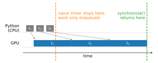
The consequence for measurement: a wall-clock timer wrapped around a GPU operation measures the enqueue, not the execution. Watch it lie:
a = torch.randn(4096, 4096, device=d2l.try_gpu(), dtype=torch.bfloat16)
b = torch.mm(a, a)  # Warmup: cuBLAS picks its kernel on first call

t0 = time.perf_counter()
for _ in range(10):
    b = torch.mm(a, a)
naive = time.perf_counter() - t0

torch.cuda.synchronize()
t0 = time.perf_counter()
for _ in range(10):
    b = torch.mm(a, a)
torch.cuda.synchronize()
honest = time.perf_counter() - t0
print(f'naive timer: {1000 * naive:.2f} ms   '
      f'with synchronize: {1000 * honest:.2f} ms')
naive timer: 0.69 ms with synchronize: 8.99 mskey = jax.random.PRNGKey(0)
a = jax.random.normal(key, (4096, 4096), dtype=jnp.bfloat16)
jnp.dot(a, a).block_until_ready() # Warmup: triggers compilation
t0 = time.perf_counter()
for _ in range(10):
b = jnp.dot(a, a)
naive = time.perf_counter() - t0
b.block_until_ready() # Drain the naive loop's in-flight work first
t0 = time.perf_counter()
for _ in range(10):
b = jnp.dot(a, a)
b.block_until_ready()
honest = time.perf_counter() - t0
print(f'naive timer: {1000 * naive:.2f} ms '
f'with block_until_ready: {1000 * honest:.2f} ms')naive timer: 0.74 ms with block_until_ready: 8.84 msThe naive timer reports close to nothing — it clocked ten kernel launches. The real number requires a barrier: in PyTorch, torch.cuda.synchronize() blocks Python until the device queue drains; in JAX, block_until_ready() blocks on one specific result (the tighter of the two — other work may proceed). Note the barrier before the second timer starts as well: without it, the naive loop’s ten still-in-flight matmuls would be billed to the synchronized loop. A measurement must both start and stop at a known-quiet device. PyTorch also offers torch.cuda.Event timestamps recorded on the device itself, which avoid stopping the pipeline at all; for whole-operation timing, synchronize-and-wall-clock gives the same answer and is what we use.
Synchronization also sneaks in where you did not ask for it. Any operation that needs a tensor’s value on the host must wait for the device to produce it:
float(x)andx.item()— converting to a Python scalar;x.cpu(),x.numpy(),np.asarray(x)— leaving device memory;print(x)— printing needs the values;- boolean control flow like
if (loss < 0.1)— deciding needs the value; - in PyTorch, shape-producing ops like
x.nonzero()— the size of the result depends on the data, so Python must wait to learn it.
Each of these is a barrier exactly like synchronize(), but implicit. The classic self-inflicted wound is reading the loss on every step of a training loop: the read itself is cheap, but it parks Python at the barrier once per step, so the GPU queue drains and the enqueue-ahead pipeline of Figure 13.1.2 never fills. Let’s measure the damage on a long chain of small operations, where staying ahead matters most:
x = torch.ones(256, 256, device=d2l.try_gpu())

torch.cuda.synchronize()
t0 = time.perf_counter()
s = 0.0
for _ in range(1000):
    y = (x * 1.01).sum()
    s += y.item()          # Reads the value: a barrier on every step
sync_every = time.perf_counter() - t0

torch.cuda.synchronize()
t0 = time.perf_counter()
s = torch.zeros((), device=d2l.try_gpu())
for _ in range(1000):
    y = (x * 1.01).sum()
    s += y                 # Accumulate on the device: no barrier
s = s.item()               # One read at the very end
sync_once = time.perf_counter() - t0
print(f'read every step: {sync_every:.3f} s   '
      f'read once: {sync_once:.3f} s')
read every step: 0.061 s read once: 0.042 sx = jnp.ones((256, 256))
t0 = time.perf_counter()
s = 0.0
for _ in range(1000):
y = (x * 1.01).sum()
s += float(y) # Reads the value: a barrier on every step
sync_every = time.perf_counter() - t0
t0 = time.perf_counter()
s = jnp.zeros(())
for _ in range(1000):
y = (x * 1.01).sum()
s = s + y # Accumulate on the device: no barrier
s = float(s) # One read at the very end
sync_once = time.perf_counter() - t0
print(f'read every step: {sync_every:.3f} s '
f'read once: {sync_once:.3f} s')read every step: 0.983 s read once: 0.361 sBoth loops launch the same kernels and compute the same total; they differ only in where the host reads. Keeping the accumulator on the device and reading once at the end cuts the wall clock by roughly a third in PyTorch and by more — around two-thirds — in JAX, where every un-jitted operation already pays a hefty dispatch cost (a preview of Section 13.3) and the per-step read stalls that pipeline on top. The exact margin is framework- and workload-dependent; the rule is not: synchronize once per minibatch at most, and only when the host actually needs the value — accumulate metrics on the device and read them at logging boundaries. (The d2l training loops used throughout this book go a step further: they hand each logged value to the plotting board, which performs the device-to-host conversion on a background thread, off the training loop.)
Since every timing in this chapter needs the same three-step discipline — warm up, synchronize, then time — we package it once. Warmup matters because first calls are unrepresentative: cuBLAS selects kernels, JAX compiles, caches fill. The class times a zero-argument callable and blocks on the device before starting and stopping the clock:
class Benchmark:
    """Time a callable: warmup, then device-synchronized average seconds."""
    def __init__(self, f, warmup=3, repeats=10, desc='time'):
        self.desc = desc
        for _ in range(warmup):
            f()
        if torch.cuda.is_available():
            torch.cuda.synchronize()
        t0 = time.perf_counter()
        for _ in range(repeats):
            f()
        if torch.cuda.is_available():
            torch.cuda.synchronize()
        self.time = (time.perf_counter() - t0) / repeats

    def __repr__(self):
        return f'{self.desc}: {1000 * self.time:.2f} ms/call'
class Benchmark:
"""Time a callable: warmup, then device-synchronized average seconds."""
def __init__(self, f, warmup=3, repeats=10, desc='time'):
self.desc = desc
for _ in range(warmup):
out = f()
jax.block_until_ready(out)
t0 = time.perf_counter()
for _ in range(repeats):
out = f()
jax.block_until_ready(out)
self.time = (time.perf_counter() - t0) / repeats
def __repr__(self):
return f'{self.desc}: {1000 * self.time:.2f} ms/call'Benchmark(lambda: torch.mm(a, a), desc='4096-matmul')4096-matmul: 0.89 ms/callBenchmark(lambda: jnp.dot(a, a), desc='4096-matmul')4096-matmul: 0.85 ms/callNote the JAX version blocks on the callable’s return value, so the callable must return what it computes — pure functions returning their results is JAX’s house style anyway, and Section 13.3 will make that convention load-bearing.
13.1.3 Throughput across Matrix Sizes
A synchronized timer lets us measure the quantity introduced at the start of this section: achieved TFLOP/s as a function of matrix size, against the roofline’s bound. A square bf16 matmul at size \(n\) performs \(2n^3\) FLOPs; its intensity \(n/3\) crosses our card’s ridge point near \(n \approx 500\), so the ceiling of Equation 13.1.2 rises for small \(n\) and flattens for large \(n\). Where the measured curve sits below that ceiling is the interesting part.
sizes = [256, 512, 1024, 2048, 4096, 8192]
achieved = []
for n in sizes:
    a = torch.randn(n, n, device=d2l.try_gpu(), dtype=torch.bfloat16)
    t = Benchmark(lambda: torch.mm(a, a)).time
    achieved.append(2 * n**3 / t / 1e12)
d2l.plot(sizes, [achieved], 'matrix size $n$', 'achieved TFLOP/s',
         xscale='log', yscale='log')
print([f'{n}: {tf:.1f}' for n, tf in zip(sizes, achieved)])
['256: 2.3', '512: 18.6', '1024: 119.6', '2048: 157.5', '4096: 152.8', '8192: 165.8']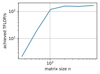
sizes = [256, 512, 1024, 2048, 4096, 8192]
achieved = []
for n in sizes:
    a = jax.random.normal(key, (n, n), dtype=jnp.bfloat16)
    compiled = jax.jit(jnp.dot).lower(a, a).compile()
    flops = compiled.cost_analysis()['flops']  # Analytic count, no timing
    t = Benchmark(lambda: compiled(a, a)).time
    achieved.append(flops / t / 1e12)
d2l.plot(sizes, [achieved], 'matrix size $n$', 'achieved TFLOP/s',
         xscale='log', yscale='log')
print([f'{n}: {tf:.1f}' for n, tf in zip(sizes, achieved)])
['256: 0.4', '512: 4.7', '1024: 21.8', '2048: 119.9', '4096: 158.7', '8192: 173.1']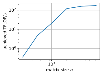
The JAX tab obtains the operation count from the compiler rather than substituting the \(2n^3\) formula. Ahead-of-time lowering (jit(...).lower(...).compile()) produces a compiled object whose cost_analysis() reports the exact analytic FLOP count of the program — no execution, no estimation. We will lean on this introspection again in Section 13.3 and Section 13.4.
Read the plot against Figure 13.1.1, remembering that the roofline is a ceiling, not a prediction of where you land. At \(n = 256\) the card delivers a percent or less of peak: the matrix is so small that per-kernel overhead (a few microseconds to launch work at all — see Section 13.2) rivals the arithmetic. More telling is \(n = 512\). Its nominal intensity (\(\approx 171\)) already sits above the ridge point, so the intensity model alone declares it compute-bound — yet the card delivers a tenth of peak or less. A \(512^2\) output provides too little work to fill 128 streaming multiprocessors, and the launch overhead has not yet been amortized away. Through the middle sizes throughput therefore climbs steeply — a single doubling of \(n\) can yield several times the TFLOP/s — and the curve approaches the specification number only around \(n \approx 2048\)–\(4096\), where the tensor cores finally saturate and the operation is compute-bound in fact as well as on paper. The nominal crossover sits at \(n \approx 500\), the measured knee at \(n \approx 2048\)–\(4096\) depending on the framework, and that gap is not a failure of the model; it is a lesson: intensity tells you when an operation stops being bandwidth-limited in principle, while utilization and overhead decide how much of the roof you collect — and separating those causes is exactly what the profiler below is for.
13.1.4 Three Regimes
The sweep distinguishes three performance regimes. Each regime requires a different optimization (He 2022). A step of any workload divides its wall-clock time among arithmetic, memory traffic, and idle gaps where the device waits for Python; whichever dominates names the regime (Figure 13.1.3).
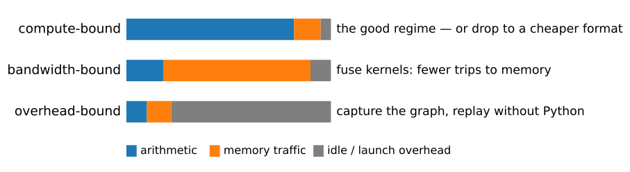
Compute-bound — arithmetic throughput is the limiting resource. Lower-precision formats may raise the applicable compute ceiling (Section 13.2, Section 13.4), while additional devices increase aggregate compute only when the parallel workload can use them (Section 13.5).
Bandwidth-bound — intensity below the ridge; the compute units remain idle while waiting for memory. The fix is to move fewer bytes: fuse chains of operations so intermediate results never make the round trip to memory (Section 13.3), recompute rather than store (Section 13.4), or restructure the algorithm for reuse — the FlashAttention kernel of Section 10.5 applies this restructuring in a specialized implementation.
Overhead-bound — the device finishes each kernel before Python can supply the next one; the GPU is idle most of the time. Small models with many small layers lie in this regime. The corresponding optimization removes Python from the launch loop: capture the whole graph once and replay it without the interpreter (Section 13.3).
A large elementwise operation provides a bandwidth-bound example. Take one large tensor and apply single elementwise kernels of wildly different arithmetic cost — an add, a multiply, and a transcendental:
x = torch.randn(4000, 4000, device=d2l.try_gpu())
for desc, f in [('add', lambda: x + 1), ('mul', lambda: x * 1.5),
                ('sin', lambda: torch.sin(x)),
                ('sigmoid', lambda: torch.sigmoid(x))]:
    print(Benchmark(f, desc=desc))
add: 0.14 ms/call
mul: 0.14 ms/call
sin: 0.14 ms/call
sigmoid: 0.14 ms/callx = jax.random.normal(key, (4000, 4000))
for desc, f in [('add', lambda: x + 1), ('mul', lambda: x * 1.5),
('sin', lambda: jnp.sin(x)),
('sigmoid', lambda: jax.nn.sigmoid(x))]:
print(Benchmark(f, desc=desc))add: 0.29 ms/call
mul: 0.30 ms/call
sin: 0.17 ms/call
sigmoid: 0.16 ms/callA sine costs far more arithmetic than an add, yet it runs no slower: each kernel’s cost is set by the 128 MB it reads and writes, not by what it computes on the way through. (In the PyTorch tab the four times are all but identical; where they scatter, as in the JAX tab, the spread is per-dispatch overhead on these un-jitted calls — a preview of the third regime — not the arithmetic.) While bandwidth is limiting, the added arithmetic does not increase elapsed time. This is the defining behavior of a bandwidth-bound operation. Now chain a few of these operations, as in any activation function or normalization layer does:
def gelu_ish(x):
    # Several elementwise ops; eager mode runs one kernel per op,
    # each a full round trip to memory
    return 0.5 * x * (1 + torch.tanh(0.8 * (x + 0.04 * x**3)))

print(Benchmark(lambda: x + 1, desc='1 op'))
print(Benchmark(lambda: gelu_ish(x), desc='chain'))
1 op: 0.14 ms/call
chain: 1.25 ms/calldef gelu_ish(x):
# Several elementwise ops; without jit, one kernel per op,
# each a full round trip to memory
return 0.5 * x * (1 + jnp.tanh(0.8 * (x + 0.04 * x**3)))
print(Benchmark(lambda: x + 1, desc='1 op'))
print(Benchmark(lambda: gelu_ish(x), desc='chain'))1 op: 0.30 ms/call
chain: 1.70 ms/callThe chain performs a handful of cheap operations, but eager execution runs each as its own kernel, and each kernel pays the full memory round trip — so the chain costs roughly as many round trips as it has operations, despite computing one output from one input. The diagnosis is complete: bandwidth-bound, with several redundant memory round trips. Section 13.3 shows how compiler fusion replaces the sequence with one kernel and verifies both numerical agreement and reduced time.
13.1.5 Profiling Complete Programs
Intensity arithmetic classifies a single operation; real training steps mix hundreds. The tool that classifies a program is the profiler, which records every kernel with its duration and stream — the measured version of Figure 13.1.2. First contact, on a small training step:
net = nn.Sequential(nn.Linear(1024, 1024), nn.ReLU(),
                    nn.Linear(1024, 1024), nn.ReLU(),
                    nn.Linear(1024, 10)).to(d2l.try_gpu())
X = torch.randn(64, 1024, device=d2l.try_gpu())
opt = torch.optim.SGD(net.parameters(), lr=0.1)

def step():
    opt.zero_grad(set_to_none=True)
    net(X).sum().backward()
    opt.step()

step()  # Warmup
with torch.profiler.profile(
        activities=[torch.profiler.ProfilerActivity.CPU,
                    torch.profiler.ProfilerActivity.CUDA],
        acc_events=True) as prof:
    for _ in range(5):
        step()
# The profiler's full table has eleven columns; we read the two that
# diagnose the regime — total CPU vs total device time, per operator.
dev = lambda e: getattr(e, 'device_time_total', 0)  # 'cuda_...' before 2.11
print(f"{'operator':<26}{'CPU total':>11}{'CUDA total':>12}")
for e in sorted(prof.key_averages(), key=dev, reverse=True)[:8]:
    print(f'{e.key[:25]:<26}{e.cpu_time_total/1e3:>8.2f} ms{dev(e)/1e3:>9.2f} ms')
operator CPU total CUDA total
aten::linear 3.21 ms 0.20 ms
aten::addmm 3.02 ms 0.20 ms
autograd::engine::evaluat 2.74 ms 0.17 ms
void cutlass::Kernel2<cut 0.00 ms 0.15 ms
AddmmBackward0 1.97 ms 0.13 ms
aten::mm 1.57 ms 0.13 ms
aten::sum 0.59 ms 0.05 ms
void cutlass::Kernel2<cut 0.00 ms 0.05 msdef loss_fn(params, X):
h = X
for W in params[:-1]:
h = jax.nn.relu(h @ W)
return (h @ params[-1]).sum()
params = [jax.random.normal(k, s) * 0.03 for k, s in zip(
jax.random.split(key, 3), [(1024, 1024), (1024, 1024), (1024, 10)])]
X = jax.random.normal(key, (64, 1024))
grad_fn = jax.jit(jax.grad(loss_fn))
jax.block_until_ready(grad_fn(params, X)) # Warmup / compile
with jax.profiler.trace('/tmp/jax-trace'):
for _ in range(5):
grads = grad_fn(params, X)
jax.block_until_ready(grads)
print('trace written to /tmp/jax-trace; '
'open it in Perfetto (ui.perfetto.dev) or TensorBoard')trace written to /tmp/jax-trace; open it in Perfetto (ui.perfetto.dev) or TensorBoardThe PyTorch table is the diagnostic in miniature. Two columns matter most: device (“CUDA”) time tells you which kernels dominate — matmuls (compute), elementwise/copy kernels (bandwidth) — and the ratio of total CPU time to total CUDA time tells you whether the GPU is fed: when CPU time is far larger, the program is overhead-bound and the kernels themselves are almost irrelevant. Read that ratio coarsely, though: CPU and device totals overlap across threads and streams, so it is a regime heuristic, not a utilization figure — when a real decision hangs on it, look at the timeline instead. Both frameworks can also export a full timeline — prof.export_chrome_trace(...) in PyTorch; the JAX trace directory above opens in Perfetto or TensorBoard — where the Figure 13.1.2 picture appears for your actual program, gaps and all. We will read one in earnest in Section 13.7.
The method. Measure with a synchronized timer or profiler. Classify the regime: compute-bound (kernels dominated by matmuls, device busy), bandwidth-bound (kernels dominated by memory traffic, device busy), or overhead-bound (device idle between kernels). Fix what binds — formats and parallelism for compute, fusion and recomputation for bandwidth, capture-and-replay for overhead. Re-measure, because the bottleneck moves. The rest of this chapter is this loop, applied.
13.1.6 Summary
- Arithmetic intensity — FLOPs per byte moved — caps performance through the roofline bound \(\min(\textrm{peak}, \textrm{intensity} \times \textrm{bandwidth})\). The ridge point of a modern GPU sits at a hundred to several hundred FLOP/byte (about 165 on our card), so most operations are bandwidth-bound, and batch size is the main natural lever on a matmul’s intensity.
- GPU dispatch is asynchronous: naive timers measure the enqueue, not the work. Time with a synchronization barrier (
torch.cuda.synchronize,block_until_ready), warm up first, and beware implicit barriers —.item(),.numpy(),print, value-dependent control flow — inside hot loops. - One matmul kernel traverses three regimes as it grows: overhead-bound when tiny, bandwidth-bound in the middle, compute-bound at scale — and it reaches the roof well after the intensity model’s nominal crossover, because small shapes cannot fill the machine. The profiler’s CPU-versus-device-time comparison diagnoses which regime a whole program is in.
- The chapter’s method: measure → classify → fix → re-measure.
13.1.7 Exercises
- The smallest dimension. The exact expression for the intensity of the product \(\mathbf{X}\mathbf{W}\) in Equation 13.1.1, the one before the approximation, holds for all shapes, not only for \(B \ll D, F\). Let \(m = \min(B, D, F)\).
- Show that the intensity lies between \(2m/(3b)\) and \(2m/b\). Conclude that in bf16, on a GPU whose ridge point is 165 FLOP/byte, every matrix product with a dimension below 165 is bandwidth-bound in the roofline model.
- Apply the bound to three bf16 products: the final layer of the MLP of Section 13.1.5, which maps width 1024 to ten outputs, on a batch of 4096 examples; the attention scores \(\mathbf{Q}\mathbf{K}^\top\) of one head with \(\mathbf{Q}, \mathbf{K} \in \mathbb{R}^{T \times 64}\) for a context of \(T\) tokens; and a \(1 \times 1\) convolution (Section 6.4.3) from 64 to 64 channels on a batch of 128 images of \(32 \times 32\) pixels. For each product, name the dimensions that would have to grow for it to reach the ridge point, and state whether a practitioner controls them.
- A multi-head attention layer computes the scores of all its heads in one batched kernel. Does batching the heads change the intensity of the scores? State what your answer implies for an attention implementation that writes the \(T \times T\) scores to memory.
- Diagnosis from timings. Suppose that
Benchmarkreports the following times per call for four operations of a bf16 program on the RTX 4090 (\(P = 165\) TFLOP/s, \(\beta = 1.008\) TB/s). Operation A multiplies two \(8192 \times 8192\) matrices in 7.4 ms. Operation B applies a softmax to the rows of an \(8192 \times 8192\) matrix in 0.30 ms; it reads and writes the matrix once and performs about five FLOPs per element. Operation C multiplies two \(256 \times 256\) matrices in 10 µs. Operation D multiplies two \(1024 \times 1024\) matrices in 40 µs.- For each operation, compute its arithmetic intensity and the fractions of \(P\) and of \(\beta\) that it achieves. Classify each operation twice: once by comparing its intensity with the ridge point, and once by the roof that it is close to. On which operations do the two classifications disagree?
- For each operation that is close to neither roof, name the most likely of the causes given in Section 13.1.3, and describe what a profiler timeline of the repeated calls would show that confirms it.
- Idle time in a profile. Suppose that two programs keep the GPU busy for only a fifth of their wall-clock time. Program A trains a small MLP with many narrow layers and launches every operation from Python. Program B trains a large convolutional network, and its data loader decodes and resizes every image in the main Python process.
- Describe where the idle gaps of each program appear in a timeline. For each program, state whether one of the fixes of the method at the end of Section 13.1.5 removes its gaps, and name that fix where one does.
- Describe an experiment that confirms the diagnosis of program B without a profiler.
- A third program keeps the GPU busy with large matrix products but converts its loss to a Python float after every step, and its profile attributes most of the host time to that conversion. Explain what the host does during that time, and why the CPU-versus-device comparison of Section 13.1.5 must not count that time as overhead.
- Intensity of a fused chain. Section 13.3.3 fuses the function
gelu_ishof Section 13.1.4 into one kernel that reads the fp32 tensorxonce and writes the result once. The elementwise arithmetic of that kernel runs on the ordinary fp32 units of the RTX 4090, at 82.6 TFLOP/s against a bandwidth of 1.008 TB/s.- Count the FLOPs per element of
gelu_ish, charging the hyperbolic tangent a few tens of FLOPs. Compute the arithmetic intensity of the fused kernel, compare it with the fp32 ridge point, and decide whether fusion moves the chain out of the bandwidth-bound regime. - Find the number of FLOPs per element at which a fused fp32 elementwise kernel with one input and one output becomes compute-bound on this GPU. What does the result imply for the speed of a fused activation function when its hyperbolic tangent is replaced by a cheaper approximation?
- Count the FLOPs per element of
- [code] Your GPU’s roofline. The sweep of Section 13.1.3 measures square bf16 matmuls on whatever GPU runs it.
- Take the dense bf16 peak and the memory bandwidth of your GPU from its specification sheet, compute its ridge point, and compute the matrix size at which the intensity \(n/3\) crosses it. Add the ceiling of Equation 13.1.2 to the plot of the sweep, and find the smallest swept size whose measured throughput reaches half of the ceiling.
- Recent NVIDIA tensor cores run fp32 matrix products in the tf32 format at half the bf16 rate. Show that the nominal crossover of the square fp32 matmul then equals that of bf16. Rerun the sweep in fp32, and compare the sizes at which the two measured curves reach half of their ceilings.
- [code] Tiles and waves. ● Model a matmul kernel on a GPU with \(S\) streaming multiprocessors (SMs, Section 13.2.3) as follows; the RTX 4090 has \(S = 128\). The kernel splits the \(n \times n\) output into \(128 \times 128\) tiles. Each SM computes one tile at a time at \(1/S\) of the peak, and the tiles run in waves of at most \(S\).
- Derive the fraction of the peak that this model allows as a function of \(n\) and \(S\), and evaluate it with the \(S\) of your GPU for the sizes of the sweep in Section 13.1.3. Compare the result with the fractions of the peak that your run of the sweep measures.
- Predict the fraction for \(n = 2176\), 2304, 2432, and 2560, all multiples of 128, relative to the fraction at \(n = 2048\). Measure the five sizes with
Benchmark, and explain where the measured pattern departs from the predicted one. - Describe two ways in which a kernel can split the product at \(n = 512\) into more pieces of work, so that all SMs take part, and state the cost that each way adds.
- [code] Batch size and the ridge. Consider the product \(\mathbf{X}\mathbf{W}\) with \(\mathbf{X} \in \mathbb{R}^{B \times 8192}\) and \(\mathbf{W} \in \mathbb{R}^{8192 \times 8192}\) in bf16.
- Using Equation 13.1.1 without the approximation, find the batch size at which the product reaches the ridge point of your GPU. Compare it with the batch size that the approximation gives.
- Predict the roofline bound on the throughput for \(B \in \{1, 8, 64, 512, 4096\}\). Measure the achieved TFLOP/s with
Benchmark, and plot the bound and the measurements against \(B\) on log-log axes. At \(B = 1\), also convert the measured time into an achieved memory bandwidth, and compare it with the specification. - When a language model generates text one token at a time, each of its linear layers runs a product of this kind with \(B\) equal to the number of sequences served together. What does your plot imply about the time per step of serving 64 sequences instead of one?
- [code] A pipeline model of dispatch. ● Model one call of a GPU operation by three durations: the host needs \(h\) to enqueue the call, the device needs \(d\) to execute it, and a barrier adds a latency \(\sigma\) after the queue drains. The device executes calls in the order in which they were enqueued, and it is idle when the first call is enqueued.
Show that \(R\) calls enqueued back to back and followed by one barrier take
\[R \max(h, d) + \min(h, d) + \sigma.\]
What does
Benchmarktherefore report for an operation with \(d < h\)? Explain why its result forx + 1on a \(256 \times 256\) tensor says nothing about the memory bandwidth of the kernel.Treat one step of the loops of Section 13.1.2 as one call. The loop that reads
yon every step waits at a barrier after each step. Express the ratio of its time to the time of the loop that accumulatesson the device in terms of \(h\), \(d\), and \(\sigma\).Run both loops with
xof side 256, 1024, 4096, and 8192. From the eight timings, estimate \(h\) and \(\sigma\), which do not depend on the size, and \(d\) for each size, and check that the model reproduces the measured ratios. Above which device time per step does reading a value on every step cost less than ten percent?
- [code] Bound versus measurement. The training step of Section 13.1.5 runs a three-layer MLP of width 1024 with ten outputs on a batch of 64 examples in fp32.
- Count the FLOPs that the matrix products of one training step perform, forward and backward, and the bytes that the step moves to read the weight matrices and write their gradients. Combine the two counts into a roofline lower bound on the device time of the step, taking the fp32 peak as the tf32 rate, half the bf16 peak.
- Time the step with
Benchmark, compare the result with the bound, and name the regime of the step.
- [extended] Roofline of a ResNet step. ● Train
ResNet18of Section 7.4 on Fashion-MNIST at \(96 \times 96\) pixels with batch size 128, as in that section, and map one training step onto the roofline of your GPU.- For every convolution of the forward pass and for the final dense layer, compute the FLOPs and the bytes, counting the input, the weights, and the output once each. Do the same for one batch normalization and one ReLU of each stage. Mark every operation at its intensity on a roofline plot of your GPU.
- Profile one training step. Split its device time among convolutions, normalizations and activations, and all other kernels, add the idle time between kernels, and report the share of each in the wall-clock time of the step.
- Apply the fix of the method that targets the largest share outside the compute-bound regime, measure again, and report which share dominates afterward.
- [code] Hidden barriers. Each of the following lines runs once per step of a training loop, where
xandgare tensors on the GPU andcis a Python float:x[x > 0].sum(),print(x.shape),x.argmax(),if g.norm() > c: g *= c / g.norm(), andx * torch.tensor(0.5, device=x.device).- Decide which of the lines make the host wait for the device, and justify each decision.
- Rewrite every line that waits so that it computes the same result without a barrier.
- Call
torch.cuda.set_sync_debug_mode('warn')before the loop, which makes PyTorch warn at every operation that synchronizes with the device, and check both answers.
- [code] Hidden barriers. Each of the following lines runs once per step of a training loop, where
xandgare arrays on the GPU andcis a Python float:x[x > 0].sum(),print(x.shape),jnp.argmax(x),if jnp.linalg.norm(g) > c: g = g * c / jnp.linalg.norm(g), andx * jnp.asarray(0.5).- Decide which of the lines make the host wait for the device, and justify each decision.
- Rewrite every line that waits so that it computes the same result without a barrier.
- Run the loop inside
with jax.transfer_guard_device_to_host('disallow'):, which raises an error at every implicit transfer of a value from the device to the host, and check both answers.