%matplotlib inline
from d2l import torch as d2l
import torch
import torchvision
from torchvision import transforms24.1 Geometry and Linear Algebraic Operations
Section 1.3 introduced the notation and operations needed to express deep learning models. Their geometric interpretation connects vectors, angles, projections, hyperplanes, and matrix transformations. We study vectors, angles, projections, hyperplanes, and the action of matrices on space. This viewpoint prepares two decompositions used in the following sections: eigendecomposition (Section 24.2) for stability, PCA, and Hessian analysis, and singular value decomposition (Section 24.3) for low-rank approximation, conditioning, and LoRA.
We first develop vector geometry and subspaces, then examine high-dimensional similarity and a linear-classifier example. Next, we interpret matrices as maps and study rank and determinants. The final part introduces tensor index notation. The part headings provide natural stopping points; later sections require the geometric and matrix-map material but not the classifier example.
24.1.1 Vectors and Their Geometry
24.1.1.1 Points and Directions
A vector admits two common geometric readings, as a point or as a direction in space. We use the following imports throughout the section.
%matplotlib inline
from d2l import tensorflow as d2l
import tensorflow as tf%matplotlib inline
from d2l import jax as d2l
import jax
from jax import numpy as jnp
import numpy as np
import tensorflow as tf%matplotlib inline
from d2l import mxnet as d2l
from mxnet import gluon, np, npx
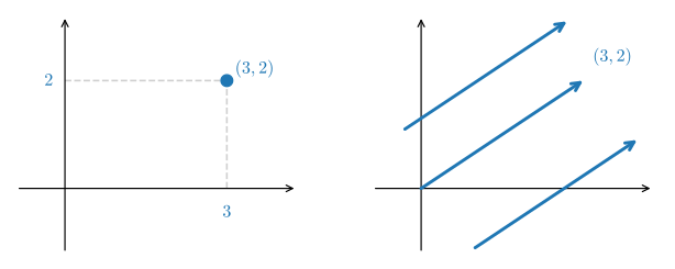
npx.set_np()Read as a point, a vector’s components give its location relative to a fixed reference called the origin: \(\mathbf{v} = [3,2]^\top\) is the point \(3\) units to the right of the origin and \(2\) units up. This reading turns a dataset into a cloud of points, and a task such as telling pictures of cats from pictures of dogs into geometry: find a way to separate two clusters of points in space.
Read as a direction, the same vector says “take \(3\) steps to the right and \(2\) steps up.” An arrow with that displacement can start anywhere, so all the parallel arrows in Figure 24.1.1 are the same vector. (On notation: a single vector is by default a column, while in a matrix holding a tabular dataset each data example is conventionally a row, as described in Section 1.3.)
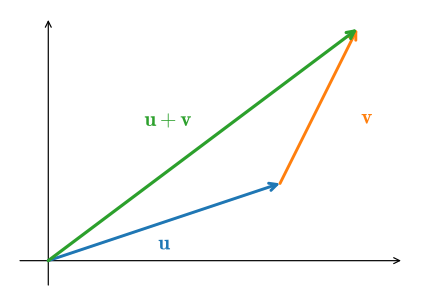
The direction view makes vector addition visual: follow one arrow, then the other, tip to tail, as in Figure 24.1.2.
Vector subtraction has a similar interpretation: from the identity \(\mathbf{u} = \mathbf{v} + (\mathbf{u}-\mathbf{v})\), the vector \(\mathbf{u}-\mathbf{v}\) is the direction that takes us from the point \(\mathbf{v}\) to the point \(\mathbf{u}\).
24.1.1.2 Dot Products and Angles
As described in Section 1.3, the dot product of two column vectors \(\mathbf{u}\) and \(\mathbf{v}\) is
\[\mathbf{u}^\top\mathbf{v} = \sum_i u_i\cdot v_i. \tag{24.1.1}\]
Because Equation 24.1.1 is symmetric, we use the notation
\[ \mathbf{u}\cdot\mathbf{v} = \mathbf{u}^\top\mathbf{v} = \mathbf{v}^\top\mathbf{u}, \]
which makes the symmetry explicit.
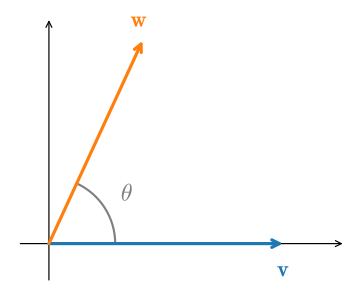
The dot product Equation 24.1.1 also has a geometric interpretation in terms of the angle between two vectors, as shown in Figure 24.1.3.
Consider two vectors
\[ \mathbf{v} = (r,0) \; \textrm{and} \; \mathbf{w} = (s\cos(\theta), s \sin(\theta)). \]
The vector \(\mathbf{v}\) is length \(r\) and runs parallel to the \(x\)-axis, and \(\mathbf{w}\) has length \(s\) and forms angle \(\theta\) with the \(x\)-axis. Their dot product is
\[ \mathbf{v}\cdot\mathbf{w} = rs\cos(\theta) = \|\mathbf{v}\|\|\mathbf{w}\|\cos(\theta). \]
For these vectors, the dot product and norms determine the angle between them. The same identity holds for any pair of vectors in a finite-dimensional space.
The first argument is purely planar. Any two vectors \(\mathbf{v}\) and \(\mathbf{w}\), however many coordinates they have, both lie in the two-dimensional plane they span, and the angle \(\theta\) between them lives in that plane. So we lose nothing by reasoning in two dimensions. Expanding \(\|\mathbf{v} - \mathbf{w}\|^2\) with the dot product gives
\[ \|\mathbf{v} - \mathbf{w}\|^2 = (\mathbf{v}-\mathbf{w})\cdot(\mathbf{v}-\mathbf{w}) = \|\mathbf{v}\|^2 - 2\,\mathbf{v}\cdot\mathbf{w} + \|\mathbf{w}\|^2, \]
while the planar law of cosines applied to the triangle with sides \(\mathbf{v}\), \(\mathbf{w}\), and \(\mathbf{v}-\mathbf{w}\) gives
\[ \|\mathbf{v} - \mathbf{w}\|^2 = \|\mathbf{v}\|^2 + \|\mathbf{w}\|^2 - 2\,\|\mathbf{v}\|\|\mathbf{w}\|\cos\theta. \]
Equating the two and cancelling \(\|\mathbf{v}\|^2 + \|\mathbf{w}\|^2\) leaves the geometric formula for the dot product,
\[ \mathbf{v}\cdot\mathbf{w} = \|\mathbf{v}\|\|\mathbf{w}\|\cos\theta, \tag{24.1.2}\]
which we may solve for the angle:
\[\theta = \arccos\left(\frac{\mathbf{v}\cdot\mathbf{w}}{\|\mathbf{v}\|\|\mathbf{w}\|}\right). \tag{24.1.3}\]
The computation is independent of the ambient dimension, so Equation 24.1.3 holds in every finite dimension.
The function \(\arccos\) is defined only on \([-1, 1]\), so Equation 24.1.3 requires its argument to lie in that interval. The following inequality provides this guarantee in every dimension.
Proposition (Cauchy–Schwarz). For any vectors \(\mathbf{v}, \mathbf{w}\),
\[ |\mathbf{v}\cdot\mathbf{w}| \le \|\mathbf{v}\|\,\|\mathbf{w}\|, \tag{24.1.4}\]
with equality if and only if \(\mathbf{v}\) and \(\mathbf{w}\) are collinear (one is a scalar multiple of the other).
Proof. If \(\mathbf{w} = \mathbf{0}\) both sides are zero and there is nothing to prove, so assume \(\mathbf{w} \neq \mathbf{0}\). Consider the squared length of \(\mathbf{v} - t\mathbf{w}\) as a function of the real number \(t\). A squared length is never negative, so
\[ q(t) = \|\mathbf{v} - t\mathbf{w}\|^2 = \|\mathbf{w}\|^2\, t^2 - 2(\mathbf{v}\cdot\mathbf{w})\, t + \|\mathbf{v}\|^2 \;\ge\; 0 \quad\textrm{for every } t. \]
This is a quadratic in \(t\) with positive leading coefficient \(\|\mathbf{w}\|^2\). A quadratic that stays non-negative cannot have two distinct real roots, so its discriminant must be \(\le 0\):
\[ \bigl(2\,\mathbf{v}\cdot\mathbf{w}\bigr)^2 - 4\,\|\mathbf{w}\|^2\,\|\mathbf{v}\|^2 \le 0, \qquad\textrm{i.e.}\qquad (\mathbf{v}\cdot\mathbf{w})^2 \le \|\mathbf{v}\|^2\,\|\mathbf{w}\|^2. \]
Taking square roots gives Equation 24.1.4. Equality forces the discriminant to vanish, which means \(q\) has a (repeated) real root \(t^\star\) with \(q(t^\star) = \|\mathbf{v} - t^\star\mathbf{w}\|^2 = 0\), that is \(\mathbf{v} = t^\star \mathbf{w}\). \(\blacksquare\)
The argument uses only the nonnegativity of a squared length. Dividing Equation 24.1.4 by \(\|\mathbf{v}\|\|\mathbf{w}\|\) for nonzero \(\mathbf{v}, \mathbf{w}\) yields the well-definedness of the angle:
\[ -1 \;\le\; \frac{\mathbf{v}\cdot\mathbf{w}}{\|\mathbf{v}\|\,\|\mathbf{w}\|} \;\le\; 1, \]
so the \(\arccos\) in Equation 24.1.3 is defined and \(\theta\) lies in \([0, \pi]\) in every dimension. The equality cases are exactly the familiar ones: \(\cos\theta = +1\) (\(\theta = 0\)) when the vectors point the same way, and \(\cos\theta = -1\) (\(\theta = \pi\)) when they point in opposite directions, precisely the collinear cases of the proposition.
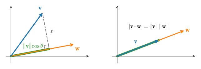
Cauchy–Schwarz also has the geometric interpretation shown in Figure 24.1.4. This picture illustrates the inequality rather than proving it, because it assumes the angle \(\theta\) and Equation 24.1.2, whose validity Cauchy–Schwarz establishes. On the left, the projection of \(\mathbf{v}\) onto \(\mathbf{w}\) has signed length \(\|\mathbf{v}\|\cos\theta\), and the residual \(\mathbf{r} = \mathbf{v} - \operatorname{proj}_{\mathbf{w}}\mathbf{v}\) meets \(\mathbf{w}\) at a right angle (we prove both facts in the next section). Because the right triangle’s hypotenuse \(\mathbf{v}\) can be no shorter than its leg, \(\|\mathbf{v}\|\,|\cos\theta| \le \|\mathbf{v}\|\), which is exactly \(|\mathbf{v}\cdot\mathbf{w}| \le \|\mathbf{v}\|\|\mathbf{w}\|\). On the right is the equality case: when \(\mathbf{v}\) is collinear with \(\mathbf{w}\) the residual vanishes and the inequality becomes an equality.
Cauchy–Schwarz immediately gives the triangle inequality, which bounds the length of a sum by the sum of the lengths.
Corollary (triangle inequality). For any \(\mathbf{v}, \mathbf{w}\), \(\|\mathbf{v} + \mathbf{w}\| \le \|\mathbf{v}\| + \|\mathbf{w}\|\).
Proof. Expand and apply Equation 24.1.4:
\[ \|\mathbf{v} + \mathbf{w}\|^2 = \|\mathbf{v}\|^2 + 2\,\mathbf{v}\cdot\mathbf{w} + \|\mathbf{w}\|^2 \le \|\mathbf{v}\|^2 + 2\,\|\mathbf{v}\|\|\mathbf{w}\| + \|\mathbf{w}\|^2 = \bigl(\|\mathbf{v}\| + \|\mathbf{w}\|\bigr)^2. \]
Taking square roots gives the claim. \(\blacksquare\)
The following function computes the angle between a pair of vectors:
import numpy as onp
def angle(v, w):
    return onp.arccos(v.dot(w) / (onp.linalg.norm(v) * onp.linalg.norm(w)))

angle(onp.array([0, 1, 2]), onp.array([2, 3, 4]))np.float64(0.4189900840328574)np.float64(0.4189900840328574)np.float64(0.4189900840328574)0.4189900840328574Two vectors whose angle is \(\pi/2\) (equivalently \(90^{\circ}\)) are called orthogonal. From Equation 24.1.2, the angle is \(\pi/2\) exactly when \(\cos\theta = 0\), and since \(\|\mathbf{v}\|\|\mathbf{w}\| \neq 0\) for nonzero vectors, this happens if and only if the dot product itself vanishes. We therefore define two vectors to be orthogonal when \(\mathbf{v}\cdot\mathbf{w} = 0\). (We take this as the definition because it extends gracefully to the zero vector, which is orthogonal to everything even though no angle is defined for it.) We will use this condition throughout the chapter.
24.1.1.3 Projection and Orthogonality
Cauchy–Schwarz answers “how aligned are two vectors?”; the closely related operation of projection answers “how much of \(\mathbf{v}\) points along \(\mathbf{w}\)?” Geometrically, we look for the point on the line \(\{t\mathbf{w} : t \in \mathbb{R}\}\) that is closest to \(\mathbf{v}\).
Proposition (orthogonal projection). Let \(\mathbf{w} \neq \mathbf{0}\). The closest multiple of \(\mathbf{w}\) to \(\mathbf{v}\) is
\[ \operatorname{proj}_{\mathbf{w}}\mathbf{v} = \frac{\mathbf{v}\cdot\mathbf{w}}{\mathbf{w}\cdot\mathbf{w}}\,\mathbf{w}, \tag{24.1.5}\]
and the residual \(\mathbf{r} = \mathbf{v} - \operatorname{proj}_{\mathbf{w}}\mathbf{v}\) is orthogonal to \(\mathbf{w}\).
Proof. We minimize the squared distance \(f(t) = \|\mathbf{v} - t\mathbf{w}\|^2 = \|\mathbf{w}\|^2 t^2 - 2(\mathbf{v}\cdot\mathbf{w})\,t + \|\mathbf{v}\|^2\). This is a convex parabola in \(t\); setting \(f'(t) = 2\|\mathbf{w}\|^2 t - 2(\mathbf{v}\cdot\mathbf{w}) = 0\) gives the unique minimizer \(t^\star = \dfrac{\mathbf{v}\cdot\mathbf{w}}{\mathbf{w}\cdot\mathbf{w}}\), which is Equation 24.1.5. For orthogonality of the residual, compute
\[ \mathbf{r}\cdot\mathbf{w} = \mathbf{v}\cdot\mathbf{w} - \frac{\mathbf{v}\cdot\mathbf{w}}{\mathbf{w}\cdot\mathbf{w}}\,(\mathbf{w}\cdot\mathbf{w}) = 0. \qquad \blacksquare \]
Because \(\mathbf{r}\) is orthogonal to \(\operatorname{proj}_{\mathbf{w}}\mathbf{v}\) (which is a multiple of \(\mathbf{w}\)), the decomposition \(\mathbf{v} = \operatorname{proj}_{\mathbf{w}}\mathbf{v} + \mathbf{r}\) splits \(\mathbf{v}\) into two perpendicular pieces, and Pythagoras applies:
\[ \|\mathbf{v}\|^2 = \|\operatorname{proj}_{\mathbf{w}}\mathbf{v}\|^2 + \|\mathbf{r}\|^2 . \tag{24.1.6}\]
Two observations connect this result to the rest of the section. First, the signed length of the projection is
\[ \frac{\mathbf{v}\cdot\mathbf{w}}{\|\mathbf{w}\|} = \|\mathbf{v}\|\cos\theta , \]
which is the quantity used in the hyperplane discussion below. Second, this is a one-dimensional least-squares problem: it finds the best approximation of \(\mathbf{v}\) from the subspace spanned by \(\mathbf{w}\). We state the general version below, as soon as the vocabulary of subspaces and bases is in hand.
24.1.1.4 Span, Bases, and Subspaces
The projection result used the one-dimensional subspace spanned by \(\mathbf{w}\), and the dot-product argument used the plane spanned by two vectors. The concepts of span, subspace, and basis organize the decompositions developed later in this chapter.
Given vectors \(\mathbf{v}_1, \ldots, \mathbf{v}_k\), their span is the set of everything reachable by scaling and adding them:
\[ \operatorname{span}(\mathbf{v}_1, \ldots, \mathbf{v}_k) = \bigl\{ a_1\mathbf{v}_1 + \cdots + a_k\mathbf{v}_k : a_1, \ldots, a_k \in \mathbb{R} \bigr\}. \]
A weighted sum \(a_1\mathbf{v}_1 + \cdots + a_k\mathbf{v}_k\) is called a linear combination, so the span is the set of all linear combinations. In \(\mathbb{R}^2\), the possibilities have a simple geometric interpretation (Figure 24.1.5): the span of a single nonzero vector is the line through the origin in its direction, while the span of two vectors that do not lie on a common line is the entire plane. A span is closed under further addition and scaling, and any set of vectors with that closure property is called a subspace. The complete list of subspaces of \(\mathbb{R}^2\) is short: the origin alone, the lines through the origin, and \(\mathbb{R}^2\) itself; in \(\mathbb{R}^3\), the planes through the origin join the list. Note that every subspace contains the origin (scale any of its elements by zero), so a line that misses the origin is not a subspace.
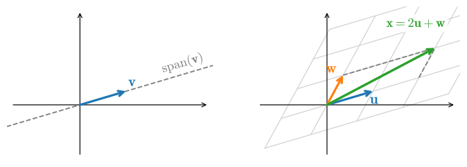
A spanning set can be redundant. If one of the vectors already lies in the span of the others, deleting it shrinks the list without shrinking the span. A collection with no such redundancy (equivalently, one where the only linear combination producing \(a_1\mathbf{v}_1 + \cdots + a_k\mathbf{v}_k = \mathbf{0}\) is the trivial one with every \(a_i = 0\)) is called linearly independent. (We return to the redundant case, linear dependence, when we study matrices and rank below.) A basis of a subspace is a linearly independent set that spans it. The coordinate vectors \(\mathbf{e}_1 = [1, 0]^\top\) and \(\mathbf{e}_2 = [0, 1]^\top\) form the standard basis of \(\mathbb{R}^2\), but the slanted pair in Figure 24.1.5 is an equally valid basis. A fundamental theorem, which we use without proof, says that every basis of a given subspace has the same number of elements and that any linearly independent set can be extended to a basis. The common count of basis elements is the subspace’s dimension. That gives, at last, a precise meaning to the \(d\) in “\(d\)-dimensional space”: \(\mathbb{R}^d\) has dimension \(d\) because \(\mathbf{e}_1, \ldots, \mathbf{e}_d\) is a basis for it.
Linear independence also guarantees unique coordinates.
Proposition (coordinates are unique). Let \(\mathbf{v}_1, \ldots, \mathbf{v}_k\) be a basis of a subspace \(S\). Then every \(\mathbf{x} \in S\) can be written as \(\mathbf{x} = a_1\mathbf{v}_1 + \cdots + a_k\mathbf{v}_k\) for exactly one choice of coefficients \(a_1, \ldots, a_k\).
Proof. At least one representation exists because the basis spans \(S\). If there were two, say \(\mathbf{x} = \sum_i a_i \mathbf{v}_i = \sum_i b_i \mathbf{v}_i\), then subtracting gives \(\sum_i (a_i - b_i)\,\mathbf{v}_i = \mathbf{0}\), and linear independence forces \(a_i = b_i\) for every \(i\). \(\blacksquare\)
A basis therefore identifies an abstract subspace with \(\mathbb{R}^k\): once the basis is fixed, the coefficient list \((a_1, \ldots, a_k)\) identifies the point. Many problems in applied linear algebra become simpler in a suitable basis. The next two sections use eigenvector and singular-vector bases for this purpose.
Finally, two subspaces attach to every matrix \(\mathbf{A}\), and they organize everything matrices do in the remainder of this chapter. The column space of \(\mathbf{A}\) is the span of its columns; since the product \(\mathbf{A}\mathbf{v}\) is exactly the linear combination of the columns of \(\mathbf{A}\) weighted by the entries of \(\mathbf{v}\) (a fact we put to work when we take up matrices as maps below), the column space is the set of all possible outputs of \(\mathbf{A}\). The null space of \(\mathbf{A}\) is the set of inputs sent to zero, \(\{\mathbf{x} : \mathbf{A}\mathbf{x} = \mathbf{0}\}\); it is a subspace because if \(\mathbf{A}\mathbf{x} = \mathbf{A}\mathbf{y} = \mathbf{0}\) then \(\mathbf{A}(a\mathbf{x} + b\mathbf{y}) = a\,\mathbf{A}\mathbf{x} + b\,\mathbf{A}\mathbf{y} = \mathbf{0}\). In words: the column space records what a matrix can produce, and the null space records what it destroys. We will measure the first when we define the rank below, and meet both again among the SVD’s four fundamental subspaces in Section 24.3.
24.1.1.5 Projection onto a Subspace
The projection proposition dropped \(\mathbf{v}\) onto a line. With subspaces and bases in hand, we can state the general version promised there: the same formula, one matrix heavier, drops a vector onto an arbitrary subspace. Call a basis \(\mathbf{q}_1, \ldots, \mathbf{q}_k\) of a subspace \(S \subseteq \mathbb{R}^n\) orthonormal when each vector has unit length and distinct vectors are orthogonal; compactly, \(\mathbf{Q}^\top\mathbf{Q} = \mathbf{I}_k\), where \(\mathbf{Q}\) is the \(n \times k\) matrix with the \(\mathbf{q}_i\) as columns.
Proposition (projection onto a subspace). Let \(\mathbf{Q}\) have orthonormal columns spanning \(S\), and set \(\mathbf{P} = \mathbf{Q}\mathbf{Q}^\top\). Then for every \(\mathbf{x} \in \mathbb{R}^n\): (i) \(\mathbf{P}\mathbf{x} \in S\), and the residual \(\mathbf{x} - \mathbf{P}\mathbf{x}\) is orthogonal to every vector of \(S\); (ii) \(\mathbf{P}\mathbf{x}\) is the unique closest point of \(S\) to \(\mathbf{x}\); (iii) \(\mathbf{P}^2 = \mathbf{P}\) and \(\mathbf{P}^\top = \mathbf{P}\).
Proof. For (i), \(\mathbf{P}\mathbf{x} = \mathbf{Q}(\mathbf{Q}^\top\mathbf{x})\) is a linear combination of the columns of \(\mathbf{Q}\), hence lies in \(S\); and \[\mathbf{Q}^\top(\mathbf{x} - \mathbf{P}\mathbf{x}) = \mathbf{Q}^\top\mathbf{x} - (\mathbf{Q}^\top\mathbf{Q})\mathbf{Q}^\top\mathbf{x} = \mathbf{0}, \tag{24.1.7}\] so the residual is orthogonal to each \(\mathbf{q}_i\) and therefore to everything they span. For (ii), take any \(\mathbf{s} \in S\) and split \(\mathbf{x} - \mathbf{s} = (\mathbf{x} - \mathbf{P}\mathbf{x}) + (\mathbf{P}\mathbf{x} - \mathbf{s})\): the second piece lies in \(S\), the first is orthogonal to it, so Pythagoras Equation 24.1.6 gives \[\|\mathbf{x} - \mathbf{s}\|^2 = \|\mathbf{x} - \mathbf{P}\mathbf{x}\|^2 + \|\mathbf{P}\mathbf{x} - \mathbf{s}\|^2 \ge \|\mathbf{x} - \mathbf{P}\mathbf{x}\|^2, \tag{24.1.8}\] with equality exactly when \(\mathbf{s} = \mathbf{P}\mathbf{x}\). For (iii), \(\mathbf{P}^2 = \mathbf{Q}(\mathbf{Q}^\top\mathbf{Q})\mathbf{Q}^\top = \mathbf{Q}\mathbf{Q}^\top = \mathbf{P}\), and symmetry is immediate from the form \(\mathbf{Q}\mathbf{Q}^\top\). \(\blacksquare\)
Property (iii) restates the geometry algebraically: projecting a second time changes nothing because the first projection already lies in \(S\). For \(k = 1\) with the single unit column \(\mathbf{q} = \mathbf{w}/\|\mathbf{w}\|\), the matrix \(\mathbf{P} = \mathbf{q}\mathbf{q}^\top\) reproduces the one-dimensional formula Equation 24.1.5 exactly.
This proposition is the geometry of least squares, the fitting problem behind linear regression. Given a data matrix \(\mathbf{A}\) whose columns are features and a target vector \(\mathbf{b}\), least squares asks for
\[ \min_{\mathbf{x}} \|\mathbf{A}\mathbf{x} - \mathbf{b}\|^2 . \tag{24.1.9}\]
As \(\mathbf{x}\) ranges over all coefficient vectors, \(\mathbf{A}\mathbf{x}\) ranges over the column space of \(\mathbf{A}\), so minimizing Equation 24.1.9 means finding the closest point to \(\mathbf{b}\) in that column space, and by property (i) the optimal residual is orthogonal to every column of \(\mathbf{A}\). The singular value decomposition solves Equation 24.1.9 in full generality in Section 24.3.
Where does an orthonormal basis come from? The library’s qr routine (the QR factorization, a matrix form of the Gram–Schmidt process we describe when we meet orthogonal matrices below) turns any full-rank matrix into one with orthonormal columns and the same column space. The following example verifies the proposition numerically on a random 3-dimensional subspace of \(\mathbb{R}^5\).
import numpy as onp
# A random 5x3 matrix whose columns span a 3-dim subspace of R^5
onp.random.seed(0)
A = onp.random.randn(5, 3)
Q, _ = onp.linalg.qr(A)  # orthonormal basis of the column space
P = Q.dot(Q.T)          # projection matrix onto that subspace
x = onp.random.randn(5)
r = x - P.dot(x)        # residual
(onp.linalg.norm(P.dot(P) - P),  # P^2 = P (idempotent)
onp.linalg.norm(Q.T.dot(r))) # residual is orthogonal to the subspace(np.float64(4.153077993666847e-16), np.float64(4.211628519682908e-16))(np.float64(4.153077993666847e-16), np.float64(4.211628519682908e-16))(np.float64(4.153077993666847e-16), np.float64(4.211628519682908e-16))(4.153077993666847e-16, 4.211628519682908e-16)Both numbers are zero up to floating-point roundoff: \(\mathbf{P}\) is idempotent, and the residual is orthogonal to the whole subspace.
24.1.2 Similarity in High Dimensions
Why is the angle, rather than the raw distance, so often the right notion of similarity? The answer is invariance to scale. Consider an image and a copy of it dimmed to \(10\%\) brightness. Pixel by pixel the two are far apart, so their Euclidean distance is large; yet the content is identical, and a cat/dog classifier should treat them the same. The angle does: for any vector \(\mathbf{v}\), the angle between \(\mathbf{v}\) and \(0.1\,\mathbf{v}\) is zero, because scaling changes a vector’s length but not its direction. This is why, when the angle is used to compare two vectors, practitioners work with its cosine and call it cosine similarity,
\[ \cos(\theta) = \frac{\mathbf{v}\cdot\mathbf{w}}{\|\mathbf{v}\|\,\|\mathbf{w}\|} \;\in\; [-1, 1], \tag{24.1.10}\]
equal to \(+1\) when the vectors point the same way, \(-1\) when opposite, and \(0\) when orthogonal. Cosine similarity is the similarity measure used for nearest-neighbor retrieval over embeddings, the scaled dot products inside attention (Section 10.2), and the alignment objective of contrastive learning (Oord et al. 2018): in each case we have represented objects as vectors and we measure relatedness by direction, deliberately discarding magnitude.
If we drop two unrelated vectors into a high-dimensional space, what cosine should we expect between them? In high dimensions, random vectors are almost always nearly orthogonal, and the higher the dimension, the more sharply this holds.
Proposition (near-orthogonality). Fix a unit vector \(\mathbf{u} \in \mathbb{R}^d\) and let \(\mathbf{v}\) be drawn uniformly from the unit sphere in \(\mathbb{R}^d\). Then \(\cos\theta = \mathbf{u}\cdot\mathbf{v}\) satisfies
\[ \mathbb{E}[\cos\theta] = 0, \qquad \operatorname{Var}(\cos\theta) = \frac{1}{d}. \]
Proof. The uniform distribution on the sphere is invariant under rotations, so we may rotate coordinates until \(\mathbf{u} = \mathbf{e}_1\); then \(\cos\theta = \mathbf{u}\cdot\mathbf{v} = v_1\). By the symmetry \(\mathbf{v} \mapsto -\mathbf{v}\) we have \(\mathbb{E}[v_1] = 0\). For the variance, every coordinate plays the same role by symmetry, so \(\mathbb{E}[v_i^2]\) is the same for all \(i\); summing and using \(\sum_i v_i^2 = \|\mathbf{v}\|^2 = 1\) gives \(d\,\mathbb{E}[v_1^2] = \mathbb{E}\!\left[\sum_i v_i^2\right] = 1\), hence \(\operatorname{Var}(\cos\theta) = \mathbb{E}[v_1^2] = 1/d\). Chebyshev’s inequality, \(\Pr(|X - \mathbb{E}X| \ge \varepsilon) \le \operatorname{Var}(X)/\varepsilon^2\) (we prove it in Section 27.1), then bounds the chance of a large cosine,
\[ \Pr\bigl(|\cos\theta| \ge \varepsilon\bigr) \le \frac{1}{d\,\varepsilon^2}, \]
which tends to \(0\) as \(d \to \infty\) for any fixed \(\varepsilon > 0\). \(\blacksquare\)
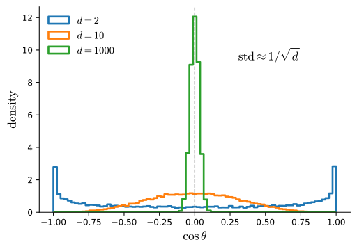
So the typical cosine between random directions has standard deviation \(1/\sqrt{d}\), concentrating ever more tightly at \(0\). This is a first taste of concentration of measure, the phenomenon that makes high-dimensional geometry behave very differently from our \(2\)- and \(3\)-dimensional intuition; we quantify it with exponential tail bounds in Section 27.6. Under this isotropic random reference model, a fixed pair has fluctuations on the scale \(1/\sqrt d\). Whether an observed cosine is unusual depends on the dimension, the number of candidates searched, and how the representations were trained; a positive cosine alone is not evidence of semantic relatedness. Embedding retrieval uses cosine similarity because training makes direction informative, not by chance.
We can watch the concentration happen by sampling random unit vectors and histogramming their pairwise cosines as the dimension grows, shown in Figure 24.1.6. Very low dimensions are genuinely different: in the plane (\(d = 2\)) the histogram piles up at \(\pm 1\) (the density is arcsine-shaped), so two random directions are more likely to be nearly aligned or nearly opposed than nearly orthogonal. Raising the dimension reverses the picture: by \(d = 10\) the histogram is a bell centered at \(0\) with standard deviation \(1/\sqrt{10} \approx 0.32\), and by \(d = 1000\) it has collapsed into a spike of width \(\approx 0.03\).
This concentration is the operating environment of dot-product attention (Section 10.2). An attention layer compares one query \(\mathbf{q}\) against thousands of keys \(\mathbf{k}_1, \mathbf{k}_2, \ldots\) by dot product. Under an isotropic reference model each unrelated score is centered at zero, although the largest among many scores need not be small. Attention learns the query and key representations; near-orthogonality alone does not guarantee separation. A short variance computation also explains the otherwise mysterious \(\sqrt{d}\) in the attention scores \(\mathbf{Q}\mathbf{K}^\top/\sqrt{d}\) (Vaswani et al. 2017). Let the query and key have independent, mean-zero, unit-variance entries. Each summand of \(\mathbf{q}\cdot\mathbf{k} = \sum_i q_i k_i\) then has mean zero and variance \(\mathbb{E}[q_i^2 k_i^2] = \mathbb{E}[q_i^2]\,\mathbb{E}[k_i^2] = 1\), and distinct summands are uncorrelated, since independence gives \(\mathbb{E}[(q_i k_i)(q_j k_j)] = 0\) for \(i \neq j\). The variances of the \(d\) summands therefore add:
\[ \operatorname{Var}(\mathbf{q}\cdot\mathbf{k}) = \sum_{i=1}^d \operatorname{Var}(q_i k_i) = d. \]
The raw scores have standard deviation \(\sqrt{d}\), growing with the dimension, and dividing by \(\sqrt{d}\) is exactly dividing by that standard deviation: it standardizes the scores to size \(O(1)\) so that the softmax downstream stays in its responsive range instead of saturating on whichever score happens to be largest (we study that softmax’s derivative in Section 25.3). The sphere proposition gives the same answer as geometric intuition: each vector has length about \(\sqrt{d}\) while the cosine between unrelated directions has typical size \(1/\sqrt{d}\), so the product lands at size \(\sqrt{d}\).
24.1.3 Hyperplanes and Decision Boundaries
A hyperplane generalizes a line in two dimensions and a plane in three dimensions. In a \(d\)-dimensional vector space, a hyperplane has \(d-1\) dimensions and divides the space into two half-spaces.
Consider a column vector \(\mathbf{w}=[2,1]^\top\) and a scalar bias \(b\). For \(b = 1\), the points \(\mathbf{v}\) satisfying \(\mathbf{w}\cdot\mathbf{v} = b\) also satisfy, by Equation 24.1.3, \[ \|\mathbf{v}\|\|\mathbf{w}\|\cos(\theta) = 1 \; \iff \; \|\mathbf{v}\|\cos(\theta) = \frac{1}{\|\mathbf{w}\|} = \frac{1}{\sqrt{5}}. \]
Thus, the signed length of the projection of \(\mathbf{v}\) onto the direction of \(\mathbf{w}\) is \(1/\|\mathbf{w}\|\); recall the signed projection length \(\|\mathbf{v}\|\cos(\theta)\) from Figure 24.1.4. These points form a line orthogonal to \(\mathbf{w}\), with equation \(2x + y = 1\), or equivalently \(y = 1 - 2x\).
More generally, the equation \(\mathbf{w}\cdot\mathbf{v} = b\) for any scalar \(b\) describes a line (in higher dimensions, a hyperplane) at right angles to \(\mathbf{w}\). The vector \(\mathbf{w}\) is called the normal to the hyperplane, and the bias \(b\) controls where along that normal the hyperplane sits. By the same projection argument, every point on it has the same signed projection \(\mathbf{w}\cdot\mathbf{v}/\|\mathbf{w}\| = b/\|\mathbf{w}\|\) onto the direction of \(\mathbf{w}\), so the hyperplane passes at (signed) distance \(b/\|\mathbf{w}\|\) from the origin. Changing \(b\) slides the hyperplane along \(\mathbf{w}\) without rotating it; the case \(b=0\) is the hyperplane through the origin. More usefully, for any point \(\mathbf{x}\) the quantity \[ \frac{\mathbf{w}\cdot\mathbf{x} - b}{\|\mathbf{w}\|} \] is the signed distance from \(\mathbf{x}\) to the hyperplane: positive on the side \(\mathbf{w}\) points toward, negative on the other, and \(0\) exactly on it. This signed distance is precisely the margin used by linear classifiers. The derivation applies the preceding projection result to the displacement of \(\mathbf{x}\) from any point on the hyperplane. These properties are illustrated in Figure 24.1.7.
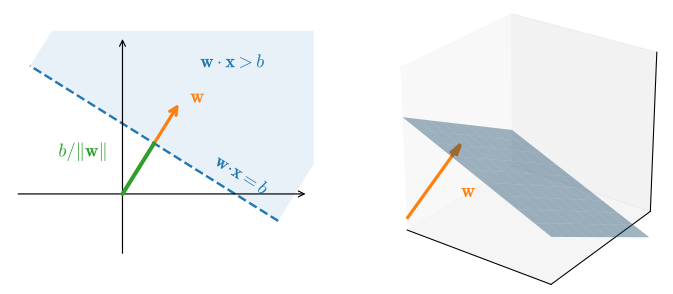
The inequalities \(\mathbf{w}\cdot\mathbf{v} > b\) and \(\mathbf{w}\cdot\mathbf{v} < b\) describe the two half-spaces. Their projections are longer or shorter than \(b/\|\mathbf{w}\|\), respectively, and their signed distances are positive and negative.
In three dimensions, for example, the points satisfying \(\mathbf{w}\cdot\mathbf{v} = b\) for \(\mathbf{w} = [1,2,3]^\top\) form a plane orthogonal to \(\mathbf{w}\), offset from the origin by the signed distance \(b/\|\mathbf{w}\|\). The two inequalities again define the two sides of the plane.
The same construction applies in any finite dimension and, with suitable extensions, in the infinite-dimensional spaces used by kernel methods. Linear classifiers such as those in Section 3.1 find hyperplanes that separate target classes. These hyperplanes are decision boundaries: the learned weight vector is the normal \(\mathbf{w}\) and the learned bias is exactly the offset \(b\), with the predicted class read off from the sign of \(\mathbf{w}\cdot\mathbf{x} - b\). Many deep classification models end with a linear layer followed by a softmax. The preceding network learns a nonlinear representation in which hyperplanes can separate the target classes.
As a simple example, we classify Fashion-MNIST images of t-shirts and trousers (Section 3.2) using the difference between their class means as the normal to a decision boundary. We first load the data and compute the means.
# Load in the dataset
trans = []
trans.append(transforms.ToTensor())
trans = transforms.Compose(trans)
train = torchvision.datasets.FashionMNIST(root="../data", transform=trans,
                                          train=True, download=True)
test = torchvision.datasets.FashionMNIST(root="../data", transform=trans,
                                         train=False, download=True)

X_train_0 = torch.stack(
    [x[0] * 255 for x in train if x[1] == 0]).type(torch.float32)
X_train_1 = torch.stack(
    [x[0] * 255 for x in train if x[1] == 1]).type(torch.float32)
X_test = torch.stack(
    [x[0] * 255 for x in test if x[1] == 0 or x[1] == 1]).type(torch.float32)
y_test = torch.stack([torch.tensor(x[1]) for x in test
                      if x[1] == 0 or x[1] == 1]).type(torch.float32)

# Compute averages
ave_0 = torch.mean(X_train_0, axis=0)
ave_1 = torch.mean(X_train_1, axis=0)
# Load in the dataset
((train_images, train_labels), (
test_images, test_labels)) = tf.keras.datasets.fashion_mnist.load_data()
X_train_0 = tf.cast(tf.stack(train_images[[i for i, label in enumerate(
train_labels) if label == 0]]), dtype=tf.float32) * 256
X_train_1 = tf.cast(tf.stack(train_images[[i for i, label in enumerate(
train_labels) if label == 1]]), dtype=tf.float32) * 256
X_test = tf.cast(tf.stack(test_images[[i for i, label in enumerate(
test_labels) if label == 0 or label == 1]]),
dtype=tf.float32) * 256
y_test = tf.cast(tf.stack([label for label in test_labels
if label == 0 or label == 1]), dtype=tf.float32)
# Compute averages
ave_0 = tf.reduce_mean(X_train_0, axis=0)
ave_1 = tf.reduce_mean(X_train_1, axis=0)# Load in the dataset
((train_images, train_labels), (
test_images, test_labels)) = tf.keras.datasets.fashion_mnist.load_data()
X_train_0 = jnp.array(train_images[train_labels == 0], dtype=jnp.float32) * 256
X_train_1 = jnp.array(train_images[train_labels == 1], dtype=jnp.float32) * 256
X_test = jnp.array(
test_images[(test_labels == 0) | (test_labels == 1)], dtype=jnp.float32) * 256
y_test = jnp.array(
test_labels[(test_labels == 0) | (test_labels == 1)], dtype=jnp.float32)
# Compute averages
ave_0 = jnp.mean(X_train_0, axis=0)
ave_1 = jnp.mean(X_train_1, axis=0)# Load in the dataset
train = gluon.data.vision.FashionMNIST(train=True)
test = gluon.data.vision.FashionMNIST(train=False)
# In MXNet 2.0 reductions over `float` (== float64) inputs stay float64, but
# many fused kernels still emit float32; pin everything to float32 up front so
# downstream dot products see matching dtypes.
X_train_0 = np.stack([x[0] for x in train if x[1] == 0]).astype('float32')
X_train_1 = np.stack([x[0] for x in train if x[1] == 1]).astype('float32')
X_test = np.stack(
[x[0] for x in test if x[1] == 0 or x[1] == 1]).astype('float32')
y_test = np.stack(
[x[1] for x in test if x[1] == 0 or x[1] == 1]).astype('float32')
# Compute averages
ave_0 = np.mean(X_train_0, axis=0)
ave_1 = np.mean(X_train_1, axis=0)The two class means are blurry but recognizable. The following plots display them side by side.
# Plot the two class means side by side
d2l.set_figsize((6, 3))
_, axes = d2l.plt.subplots(1, 2)
axes[0].imshow(ave_0.reshape(28, 28).tolist(), cmap='Greys')
axes[0].set_title('mean t-shirt')
axes[1].imshow(ave_1.reshape(28, 28).tolist(), cmap='Greys')
axes[1].set_title('mean trousers')
d2l.plt.show()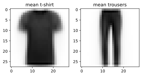
# Plot the two class means side by side
d2l.set_figsize((6, 3))
_, axes = d2l.plt.subplots(1, 2)
axes[0].imshow(tf.reshape(ave_0, (28, 28)), cmap='Greys')
axes[0].set_title('mean t-shirt')
axes[1].imshow(tf.reshape(ave_1, (28, 28)), cmap='Greys')
axes[1].set_title('mean trousers')
d2l.plt.show()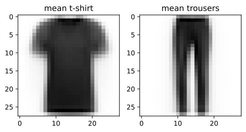
# Plot the two class means side by side
d2l.set_figsize((6, 3))
_, axes = d2l.plt.subplots(1, 2)
axes[0].imshow(np.array(ave_0.reshape(28, 28)), cmap='Greys')
axes[0].set_title('mean t-shirt')
axes[1].imshow(np.array(ave_1.reshape(28, 28)), cmap='Greys')
axes[1].set_title('mean trousers')
d2l.plt.show()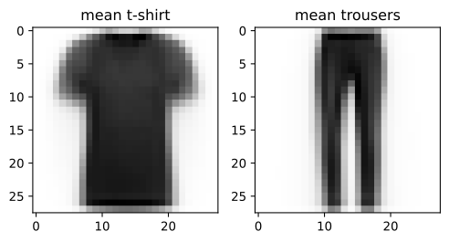
# Plot the two class means side by side
d2l.set_figsize((6, 3))
_, axes = d2l.plt.subplots(1, 2)
axes[0].imshow(ave_0.reshape(28, 28).tolist(), cmap='Greys')
axes[0].set_title('mean t-shirt')
axes[1].imshow(ave_1.reshape(28, 28).tolist(), cmap='Greys')
axes[1].set_title('mean trousers')
d2l.plt.show()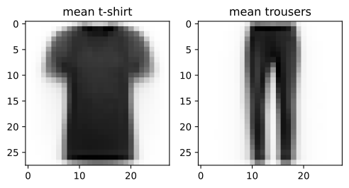
In a fully learned solution, the threshold would be estimated from the dataset. Here we set it geometrically instead: the normal is the difference of the two class means \(\mathbf{w} = \overline{\mathbf{x}}_1 - \overline{\mathbf{x}}_0\), and the natural decision boundary is the hyperplane that bisects the two means: \(\mathbf{w}\cdot\mathbf{x} = b\) with \(b = \mathbf{w}\cdot\tfrac12(\overline{\mathbf{x}}_0 + \overline{\mathbf{x}}_1)\), the midpoint of the two means’ projections onto \(\mathbf{w}\). We classify a test image as class \(1\) when it lands on the class-\(1\) side, i.e. \(\mathbf{w}\cdot\mathbf{x} > b\). Deriving \(b\) from the data this way is scale-equivariant: it gives the same boundary whatever convention each framework uses for pixel intensities, which a hand-picked numeric threshold would not.
import numpy as onp
def as_numpy(x):
    if hasattr(x, 'asnumpy'):                   # MXNet
        return x.asnumpy()
    if hasattr(x, 'detach'):                    # PyTorch
        return x.detach().cpu().numpy()
    if hasattr(x, 'numpy'):                     # TensorFlow
        return x.numpy()
    return onp.asarray(x)                       # JAX / NumPy

X_test_np, y_test_np = as_numpy(X_test), as_numpy(y_test)
ave_0_np, ave_1_np = as_numpy(ave_0), as_numpy(ave_1)
# Normal = difference of class means; threshold = midpoint of their projections
w = (ave_1_np - ave_0_np).ravel()
b = onp.dot(w, (ave_0_np + ave_1_np).ravel()) / 2
predictions = X_test_np.reshape(len(X_test_np), -1).dot(w) > b

# Accuracy
onp.mean(predictions.astype(y_test_np.dtype) == y_test_np, dtype=onp.float64)np.float64(0.9155)np.float64(0.9155)np.float64(0.9155)0.922In this run, the rule classifies about \(92\%\) of the \(2{,}000\) test images correctly without iterative parameter training. We computed two class means, took their difference as the normal \(\mathbf{w}\), and asked of each test image only which side of one hyperplane its \(784\)-dimensional pixel vector lies on. To see the geometry of why such a crude rule works, project every test image onto the normal: reduce each image to the single number \(\mathbf{w}\cdot\mathbf{x}\), its (scaled) signed position along the direction from “mean t-shirt” to “mean trousers”, and histogram the two classes separately.
import numpy as onp
# Histogram of the test images' projections onto the normal direction w
proj = X_test_np.reshape(len(X_test_np), -1).dot(w)
d2l.set_figsize()
d2l.plt.hist(proj[y_test_np == 0], bins=50, alpha=0.6, label='t-shirts')
d2l.plt.hist(proj[y_test_np == 1], bins=50, alpha=0.6, label='trousers')
d2l.plt.axvline(float(b), color='black', linestyle='--', label='threshold')
d2l.plt.xlabel(r'$\mathbf{w}\cdot\mathbf{x}$')
d2l.plt.legend()
d2l.plt.show()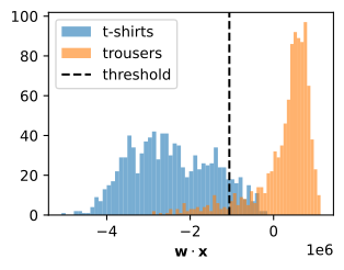
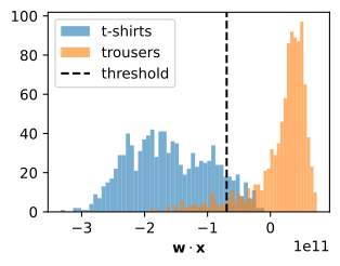
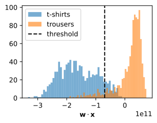
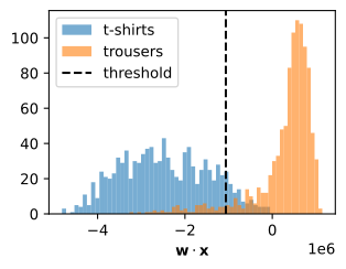
This plot summarizes the geometry of hyperplane classifiers. Along the single direction \(\mathbf{w}\), the two classes form two well-separated modes, and the dashed threshold cuts between them, at the value \(\mathbf{w}\cdot\mathbf{x}\) takes at the midpoint of the two means; the tails that spill across it are exactly the \(\approx 8\%\) of images the rule misclassifies. A learned linear classifier, such as the softmax regression of Section 3.1, improves on this only by moving and tilting the same kind of boundary to reduce the overlap. A deep network also learns a representation in which the class distributions are more readily separated by a hyperplane.
24.1.4 Matrices as Linear Maps
24.1.4.1 Linear Transformations
As introduced in Section 1.3, matrices represent linear transformations. We now study their geometry, using two dimensions for visualization.
Consider the matrix
\[ \mathbf{A} = \begin{bmatrix} a & b \\ c & d \end{bmatrix}. \]
Applying it to an arbitrary vector \(\mathbf{v} = [x, y]^\top\) gives
\[ \begin{aligned} \mathbf{A}\mathbf{v} & = \begin{bmatrix}a & b \\ c & d\end{bmatrix}\begin{bmatrix}x \\ y\end{bmatrix} & = \begin{bmatrix}ax+by\\ cx+dy\end{bmatrix} \\ & = x\begin{bmatrix}a \\ c\end{bmatrix} + y\begin{bmatrix}b \\d\end{bmatrix} & = x\left\{\mathbf{A}\begin{bmatrix}1\\0\end{bmatrix}\right\} + y\left\{\mathbf{A}\begin{bmatrix}0\\1\end{bmatrix}\right\}. \end{aligned} \]
This calculation expresses the image of any vector in terms of the images of two specific vectors, \([1,0]^\top\) and \([0,1]^\top\). The vectors \([1,0]^\top\) and \([0,1]^\top\) are exactly the standard basis \(\mathbf{e}_1, \mathbf{e}_2\) from our discussion of spans and bases: because every vector is a (unique) weighted sum of basis vectors, knowing where a matrix sends a basis determines where it sends everything.
Consider the specific matrix
\[ \mathbf{A} = \begin{bmatrix} 1 & 2 \\ -1 & 3 \end{bmatrix}. \]
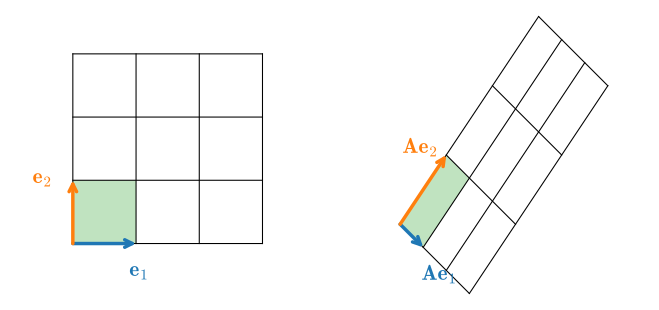
The vector \(\mathbf{v} = [2, -1]^\top\) equals \(2\cdot[1,0]^\top - [0,1]^\top\), so \(\mathbf{A}\) maps it to \(2\,\mathbf{A}[1,0]^\top - \mathbf{A}[0,1]^\top = 2[1, -1]^\top - [2,3]^\top = [0, -5]^\top\). Applying the same reasoning to the integer grid shows that matrix multiplication can shear, rotate, reflect, project, and scale directions while preserving linear combinations, as shown in Figure 24.1.8.
The defining restriction is position-independent linearity: the same displacement is transformed identically everywhere, and linear combinations are preserved.
Some distortions can be severe. For instance the matrix
\[ \mathbf{B} = \begin{bmatrix} 2 & -1 \\ 4 & -2 \end{bmatrix}, \]
compresses the entire two-dimensional plane down to a single line. Such transformations differ fundamentally from invertible maps. The image of \(\mathbf{A}\) can be mapped back to the original grid, whereas \(\mathbf{B}\) maps distinct inputs to the same output. For example, both \([1,1]^\top\) and \([0, -1]^\top\) map to \([1,2]^\top\).
The same reasoning extends beyond \(2\times2\) matrices. In any dimension, the images of the basis vectors determine the action of the matrix on the entire space. For example, \([1,0, \ldots,0]\) selects the first column.
Nothing requires the matrix to be square, either. An \(m \times n\) matrix takes vectors with \(n\) entries to vectors with \(m\) entries: it is a linear map between spaces, from \(\mathbb{R}^n\) to \(\mathbb{R}^m\), and it is still determined by where it sends the \(n\) basis vectors (whose images are its columns). A \(2 \times 3\) matrix has an image of dimension at most two; it fills the output plane only when its rank is two. A \(3 \times 2\) matrix has a plane through the origin as its image when its rank is two, and a line or the origin at lower rank. Every fully connected layer of a neural network is such a map between spaces of different dimensions, composed with a nonlinearity.
24.1.4.2 Orthogonal Matrices
A matrix may skew, rotate, and scale, but a special family does only the rigid part: it rotates or reflects without any stretching. A square matrix \(\mathbf{Q}\) is called orthogonal when its columns are orthonormal, which we can write compactly as \(\mathbf{Q}^\top\mathbf{Q} = \mathbf{I}\). The defining property of such maps is that they preserve lengths and angles, because they preserve every dot product:
\[ (\mathbf{Q}\mathbf{x})\cdot(\mathbf{Q}\mathbf{y}) = (\mathbf{Q}\mathbf{x})^\top(\mathbf{Q}\mathbf{y}) = \mathbf{x}^\top\mathbf{Q}^\top\mathbf{Q}\,\mathbf{y} = \mathbf{x}^\top\mathbf{y} = \mathbf{x}\cdot\mathbf{y}. \]
Taking \(\mathbf{y} = \mathbf{x}\) shows \(\|\mathbf{Q}\mathbf{x}\| = \|\mathbf{x}\|\), so an orthogonal map is a rigid motion of space. Since \(\mathbf{Q}^\top\mathbf{Q} = \mathbf{I}\) means \(\mathbf{Q}^{-1} = \mathbf{Q}^\top\), such maps are invertible, and as we will prove when we meet the determinant at the end of this section, their volume scaling is \(\det\mathbf{Q} = \pm 1\) (the sign distinguishes orientation-preserving from orientation-reversing maps). Orthogonal matrices preserve lengths and angles, and they will turn out to be the building blocks of the two decompositions in the sections that follow: the spectral theorem writes a symmetric matrix as \(\mathbf{Q}\boldsymbol\Lambda\mathbf{Q}^\top\) (Section 24.2), and the singular value decomposition writes any matrix as orthogonal–diagonal–orthogonal (Section 24.3).
Where do orthonormal columns come from in the first place? Any linearly independent collection can be converted into an orthonormal basis of its span by the Gram–Schmidt process: process the vectors in order, subtract from each one its projection Equation 24.1.5 onto each direction already produced, and normalize what remains. In matrix form this algorithm is the QR factorization, the qr call that produced the orthonormal basis in our subspace-projection demo earlier in this section. We will not need its inner workings in this chapter; it is enough to know that orthonormal bases can be computed by standard numerical routines, which makes decompositions built from them practical.
24.1.4.3 Linear Dependence, Rank, and Invertibility
Consider again the matrix
\[ \mathbf{B} = \begin{bmatrix} 2 & -1 \\ 4 & -2 \end{bmatrix}. \]
This maps the entire plane to the single line \(y = 2x\), a property visible from the matrix itself. Let \(\mathbf{b}_1 = [2,4]^\top\) and \(\mathbf{b}_2 = [-1, -2]^\top\) denote the two columns of \(\mathbf{B}\). Every output of \(\mathbf{B}\) is a linear combination \(a_1\mathbf{b}_1 + a_2\mathbf{b}_2\); in the language of spans, the outputs of \(\mathbf{B}\) fill out exactly its column space. The fact that \(\mathbf{b}_1 = -2\cdot\mathbf{b}_2\) means that we can write any linear combination of those two columns entirely in terms of say \(\mathbf{b}_2\) since
\[ a_1\mathbf{b}_1 + a_2\mathbf{b}_2 = -2a_1\mathbf{b}_2 + a_2\mathbf{b}_2 = (a_2-2a_1)\mathbf{b}_2. \]
Thus, one column is redundant, consistent with the collapse of the plane to a line. The dependence \(\mathbf{b}_1 = -2\cdot\mathbf{b}_2\) can be written symmetrically as
\[ \mathbf{b}_1 + 2\cdot\mathbf{b}_2 = 0. \]
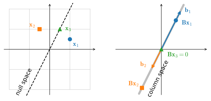
The coefficients \((1, 2)\) of this relation say precisely that \(\mathbf{B}[1, 2]^\top = 1\cdot\mathbf{b}_1 + 2\cdot\mathbf{b}_2 = \mathbf{0}\), so the dependence hands us a nonzero vector in the null space of \(\mathbf{B}\). Figure 24.1.9 shows the two subspaces of \(\mathbf{B}\) together: the whole plane is mapped onto the column space, while the null-space direction is exactly the set of inputs that land on the origin. (For this particular \(\mathbf{B}\) the two subspaces happen to coincide as sets, both being the line \(y = 2x\): a coincidence, equivalent to \(\mathbf{B}^2 = \mathbf{0}\), that makes the picture no less instructive, since what the matrix produces and what it destroys are different roles even when they occupy the same line.)
In general, we will say that a collection of vectors \(\mathbf{v}_1, \ldots, \mathbf{v}_k\) are linearly dependent if there exist coefficients \(a_1, \ldots, a_k\) not all equal to zero so that
\[ \sum_{i=1}^k a_i\mathbf{v}_i = 0. \]
In this case, one vector can be expressed as a combination of the others and is therefore redundant. Linear dependence among the columns shows that the matrix maps the input space to a lower-dimensional subspace. If there is no linear dependence we say the vectors are linearly independent, the same notion we met when defining bases, now read as a property of a matrix’s columns. If a matrix has linearly independent columns, the map is injective and its inputs can be recovered from outputs in its image. A square such matrix is invertible.
24.1.4.3.1 Rank
For a general \(m\times n\) matrix, the rank is the dimension of its image. Equivalently, the rank of \(\mathbf{A}\) is the largest number of linearly independent columns amongst all subsets of columns. For example, our matrix
\[ \mathbf{B} = \begin{bmatrix} 2 & -1 \\ 4 & -2 \end{bmatrix} \]
from above has \(\textrm{rank}(\mathbf{B})=1\), since the two columns \([2, 4]^\top\) and \([-1, -2]^\top\) are linearly dependent, while each column on its own is linearly independent. As another example, consider
\[ \mathbf{C} = \begin{bmatrix} 1& 3 & 0 & -1 & 0 \\ -1 & 0 & 1 & 1 & -1 \\ 0 & 3 & 1 & 0 & -1 \\ 2 & 3 & -1 & -2 & 1 \end{bmatrix}, \]
and show that \(\mathbf{C}\) has rank two since, for instance, the first two columns are linearly independent, however any of the \(\binom{5}{3} = 10\) collections of three columns are linearly dependent. (Exercise: verify this, either by hand or with matrix_rank.)
Equivalently, the rank is the dimension of the column space we defined alongside spans and bases, and a foundational theorem of linear algebra says this equals the dimension of the row space, the span of the rows. A matrix “compresses space” into a lower dimension exactly when its rank is smaller than its number of columns, equivalently, when its null space contains some nonzero vector.
Checking every subset of columns is potentially exponential in the number of columns. Later sections introduce more efficient ways to compute rank; the subset definition is useful here for establishing its meaning.
Rank–nullity quantifies the dimensions mapped to zero and retained in the image.
Proposition (rank–nullity). For an \(m \times n\) matrix \(\mathbf{A}\),
\[ \operatorname{rank}\mathbf{A} + \dim\ker\mathbf{A} = n, \]
where \(\ker\mathbf{A}\) denotes the null space.
Proof. Choose a basis \(\mathbf{w}_1, \ldots, \mathbf{w}_k\) of the null space and extend it to a basis \(\mathbf{w}_1, \ldots, \mathbf{w}_k, \mathbf{v}_1, \ldots, \mathbf{v}_{n-k}\) of \(\mathbb{R}^n\). The images \(\mathbf{A}\mathbf{v}_1, \ldots, \mathbf{A}\mathbf{v}_{n-k}\) span the column space (the \(\mathbf{w}_i\) contribute nothing), and they are independent: if \(\sum_i c_i \mathbf{A}\mathbf{v}_i = \mathbf{0}\) then \(\sum_i c_i \mathbf{v}_i\) lies in the null space, hence is a combination of the \(\mathbf{w}_j\), impossible within a basis unless every \(c_i = 0\). So the column space has dimension exactly \(n - k\). \(\blacksquare\)
Of the \(n\) input dimensions, \(\dim\ker\mathbf{A}\) map to zero and \(\operatorname{rank}\mathbf{A}\) remain in the image. For \(\mathbf{B}\) the count is \(1 + 1 = 2\): the column space and null space each have dimension one, as Figure 24.1.9 shows. The singular value decomposition will make this split visible, with orthonormal bases attached to both halves, in Section 24.3.
24.1.4.3.2 Invertibility
A matrix with linearly dependent columns maps some distinct inputs to the same output, so no inverse can recover every input. By contrast, a square full-rank matrix \(\mathbf{A}\) of size \(n \times n\) is both injective and surjective and therefore invertible. Consider the matrix
\[ \mathbf{I} = \begin{bmatrix} 1 & 0 & \cdots & 0 \\ 0 & 1 & \cdots & 0 \\ \vdots & \vdots & \ddots & \vdots \\ 0 & 0 & \cdots & 1 \end{bmatrix}. \]
This identity matrix has ones on the diagonal and zeros elsewhere, and it leaves every vector unchanged. An inverse of \(\mathbf{A}\) is a matrix \(\mathbf{A}^{-1}\) satisfying
\[ \mathbf{A}^{-1}\mathbf{A} = \mathbf{A}\mathbf{A}^{-1} = \mathbf{I}. \]
Viewed entrywise, \(\mathbf{A}^{-1}\) has \(n \times n\) unknown entries, and the product \(\mathbf{A}^{-1}\mathbf{A}\) must equal \(\mathbf{I}\), imposing \(n \times n\) scalar constraints. Their number alone does not guarantee a solution; full rank does. When it exists, \(\mathbf{A}^{-1}\) is unique for an \(n\)-dimensional square map.
The determinant, introduced below, gives an equivalent criterion: the inverse exists exactly when the determinant is nonzero. As an example, if \(\mathbf{A}\) is the general \(2 \times 2\) matrix
\[ \mathbf{A} = \begin{bmatrix} a & b \\ c & d \end{bmatrix}, \]
then its inverse is
\[ \frac{1}{ad-bc} \begin{bmatrix} d & -b \\ -c & a \end{bmatrix}. \]
The following multiplication verifies the formula for a specific matrix.
import numpy as onp
M = onp.array([[1, 2], [1, 4]])
M_inv = onp.array([[2, -1], [-0.5, 0.5]])
M_inv.dot(M)
array([[1., 0.],
[0., 1.]])24.1.4.3.3 Numerical Issues
While the matrix inverse is useful in theory, in practice we rarely want to compute it. To solve the linear system \(\mathbf{A}\mathbf{x} = \mathbf{b}\), prefer linalg.solve(A, b) to the tempting but inferior inv(A) @ b: the solver factorizes \(\mathbf{A}\) without ever forming its inverse. Like division by a small number, inversion of a matrix that is close to having low rank can amplify numerical errors. Sparsity raises the stakes further. A matrix with a million rows and columns but only \(5\) million non-zero entries is cheap to store, yet its inverse is typically dense, with on the order of \(10^{12}\) non-zero entries. The condition number of Section 24.3.3.2 makes “close to low rank” precise, and measures exactly how much a solve can amplify error.
24.1.4.4 The Determinant
The geometric view gives an intuitive interpretation of the determinant. Return to the grid picture of Figure 24.1.8 and watch the shaded unit square, the square with edges \(\mathbf{e}_1 = (1,0)^\top\) and \(\mathbf{e}_2 = (0,1)^\top\), hence with area one. The matrix
\[ \mathbf{A} = \begin{bmatrix} 1 & 2 \\ -1 & 3 \end{bmatrix} \]
carries it to the shaded parallelogram with edges \(\mathbf{A}\mathbf{e}_1 = [1, -1]^\top\) and \(\mathbf{A}\mathbf{e}_2 = [2, 3]^\top\). There is no reason this parallelogram should have the same area that we started with, and indeed an exercise in coordinate geometry shows that its area is exactly \(5\): this particular matrix quintuples areas.
In general, a matrix
\[ \mathbf{A} = \begin{bmatrix} a & b \\ c & d \end{bmatrix} \]
sends the unit square to the parallelogram with edges \((a, c)^\top\) and \((b, d)^\top\), and we can compute that parallelogram’s area directly. Suppose for the moment that all four entries are positive and that \((a, c)^\top\) makes the smaller angle with the \(x\)-axis. The parallelogram has vertices \((0,0)\), \((a, c)\), \((b, d)\), and \((a+b, c+d)\); enclose it in its bounding rectangle \([0, a+b] \times [0, c+d]\). The part of the rectangle outside the parallelogram consists of two \(b \times c\) rectangles in the corners, two right triangles with legs \(a\) and \(c\), and two right triangles with legs \(b\) and \(d\). Subtracting all six pieces from the rectangle’s area leaves
\[ (a+b)(c+d) - 2bc - 2\cdot\tfrac{1}{2}\,ac - 2\cdot\tfrac{1}{2}\,bd = ad - bc. \]
Working through the other sign configurations changes only the sign of the result, never its magnitude: the parallelogram’s area is always \(|ad - bc|\). The signed quantity \(ad-bc\) is referred to as the determinant, written \(\det\mathbf{A}\).
The following code confirms the worked example: for the matrix \(\mathbf{A}\) above the determinant should come out to \(1 \cdot 3 - 2 \cdot (-1) = 5\).
import numpy as onp
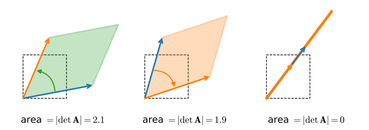
onp.linalg.det(onp.array([[1, 2], [-1, 3]]))np.float64(4.999999999999999)np.float64(4.999999999999999)np.float64(4.999999999999999)4.999999999999999The expression \(ad - bc\) can be zero or negative, and Figure 24.1.10 shows the three possible regimes side by side, each for a different matrix: a positive determinant, where the unit square maps to a parallelogram of area \(\det\mathbf{A}\); a negative determinant, where the parallelogram has area \(|\det\mathbf{A}|\) but the map has flipped the orientation of the plane (the images of \(\mathbf{e}_1\) and \(\mathbf{e}_2\) have traded sides); and a zero determinant, where the square is mapped to a segment. The sign convention records an orientation reversal as a negative signed area.
A zero determinant reveals a loss of dimension. Consider the matrix
\[ \mathbf{B} = \begin{bmatrix} 2 & -1 \\ 4 & -2 \end{bmatrix}. \]
If we compute the determinant of this matrix, we get \(2\cdot(-2) - (-1)\cdot 4 = 0\). \(\mathbf{B}\) compresses the unit square down to a segment of the line \(y = 2x\), which has zero area: the situation of panel (c) in Figure 24.1.10, and exactly the collapse pictured in Figure 24.1.9. And indeed, being compressed into a lower dimensional space is the only way to have zero area after the transformation. Thus, a square matrix \(A\) is invertible if and only if the determinant is not equal to zero. We prove this equivalence below, once the determinant exists in every dimension.
24.1.4.4.1 The Determinant in General
The two-dimensional picture says what the determinant of an \(n \times n\) matrix should be: the signed volume of the parallelepiped spanned by its columns. Rather than wrestle with \(n\)-dimensional geometry directly, we distill the three properties of signed volume that determine it completely, stated for the columns \(\mathbf{a}_1, \ldots, \mathbf{a}_n\) of an \(n \times n\) matrix:
- Multilinear: \(\det\) is linear in each column separately, with the other columns held fixed. (Scaling one edge of a parallelepiped scales its volume; splitting one edge as a sum splits the volume accordingly.)
- Alternating: \(\det\) is zero whenever two columns are equal. (The parallelepiped then flattens into a lower-dimensional slab of zero volume.)
- Normalized: \(\det \mathbf{I} = 1\). (The unit cube has volume one.)
We grant one fact here without proof: exactly one function of the columns has these three properties, and it is the determinant (see (Horn and Johnson 2012) for the construction and the uniqueness argument). Uniqueness comes in a sharper form that we will use below: every function \(f\) of the columns satisfying (1) and (2) is a multiple of the determinant, \(f = f(\mathbf{I}) \cdot \det\). To see why, set \(g = f - f(\mathbf{I})\cdot\det\); then \(g\) satisfies (1) and (2) with \(g(\mathbf{I}) = 0\), so \(g + \det\) satisfies all three properties, hence equals \(\det\) by uniqueness, forcing \(g = 0\).
The three properties yield several useful identities. First, swapping two columns flips the sign of the determinant. Place the vector \(\mathbf{u}+\mathbf{v}\) in two different column slots and expand by multilinearity:
\[ \begin{aligned} 0 &= \det(\ldots, \mathbf{u}+\mathbf{v}, \ldots, \mathbf{u}+\mathbf{v}, \ldots) \\ &= \det(\ldots, \mathbf{u}, \ldots, \mathbf{u}, \ldots) + \det(\ldots, \mathbf{u}, \ldots, \mathbf{v}, \ldots) + \det(\ldots, \mathbf{v}, \ldots, \mathbf{u}, \ldots) + \det(\ldots, \mathbf{v}, \ldots, \mathbf{v}, \ldots). \end{aligned} \]
The left-hand side, the first term, and the last term all vanish by the alternating property, leaving
\[ \det(\ldots, \mathbf{u}, \ldots, \mathbf{v}, \ldots) = -\det(\ldots, \mathbf{v}, \ldots, \mathbf{u}, \ldots). \]
This is where the sign of the signed area comes from: exchanging two edges reverses the orientation of the parallelepiped, and an odd permutation of the columns negates the determinant.
Second, the three properties pin down a formula. Expand each column in the standard basis, \(\mathbf{a}_j = \sum_i a_{ij}\,\mathbf{e}_i\), and apply multilinearity column by column: \(\det\mathbf{A}\) becomes a sum of terms of the form \(a_{i_1 1} a_{i_2 2} \cdots a_{i_n n} \det(\mathbf{e}_{i_1}, \ldots, \mathbf{e}_{i_n})\). Whenever two of the chosen row indices coincide, the term vanishes by the alternating property; when all are distinct, the columns \(\mathbf{e}_{i_1}, \ldots, \mathbf{e}_{i_n}\) are a reshuffling of the identity matrix’s, so repeated column swaps reduce the determinant factor to \(\pm 1\). For a \(2 \times 2\) matrix with columns \(\mathbf{a}_1 = a\,\mathbf{e}_1 + c\,\mathbf{e}_2\) and \(\mathbf{a}_2 = b\,\mathbf{e}_1 + d\,\mathbf{e}_2\), the expansion has four terms; the two with a repeated basis vector vanish and
\[ \det(\mathbf{a}_1, \mathbf{a}_2) = ad\,\det(\mathbf{e}_1, \mathbf{e}_2) + cb\,\det(\mathbf{e}_2, \mathbf{e}_1) = ad - bc, \]
recovering the parallelogram area we computed by hand. In general the determinant is a signed sum of the products of the chosen entries, taken over all ways of picking one entry from each row and each column; this is the permutation formula, and (1)+(2)+(3) leave no other possibility.
For hand computation the sum is organized as cofactor expansion: expanding the first column in the standard basis splits \(\det\mathbf{A}\) into \(n\) smaller determinants, with alternating signs, of the submatrices obtained by deleting the first column and one row. Consider the \(3 \times 3\) example
\[ \mathbf{A} = \begin{bmatrix} 2 & 1 & 0 \\ 1 & 3 & 1 \\ 0 & 1 & 2 \end{bmatrix}, \]
expanding along the first column:
\[ \det \mathbf{A} = 2 \det \begin{bmatrix} 3 & 1 \\ 1 & 2 \end{bmatrix} - 1 \det \begin{bmatrix} 1 & 0 \\ 1 & 2 \end{bmatrix} + 0 \det \begin{bmatrix} 1 & 0 \\ 3 & 1 \end{bmatrix} = 2 \cdot 5 - 1 \cdot 2 + 0 = 8. \tag{24.1.11}\]
Geometrically, \(\mathbf{A}\) maps the unit cube to a parallelepiped of volume \(8\), and it scales the volume of every solid by that same factor. The following code checks Equation 24.1.11 and two consequences of the properties above: swapping two columns flips the sign, and the determinant of a triangular matrix is the product of its diagonal entries.
import numpy as onp
A = onp.array([[2, 1, 0], [1, 3, 1], [0, 1, 2]])
A_swap = onp.array([[1, 2, 0], [3, 1, 1], [1, 0, 2]])  # first two columns swapped
T = onp.array([[2, 5, 1], [0, 3, 4], [0, 0, 1]])       # upper triangular
(onp.linalg.det(A),       # 8, matching the cofactor expansion
 onp.linalg.det(A_swap),  # -8: a column swap flips the sign
onp.linalg.det(T)) # 6 = 2 * 3 * 1, the diagonal product(np.float64(8.000000000000002),
np.float64(-8.000000000000002),
np.float64(6.0))(np.float64(8.000000000000002),
np.float64(-8.000000000000002),
np.float64(6.0))(np.float64(8.000000000000002),
np.float64(-8.000000000000002),
np.float64(6.0))(8.000000000000002, -8.000000000000002, 6.0)The triangular rule deserves its one-paragraph proof, since the next section relies on it. Suppose \(\mathbf{T}\) is upper triangular, so \(t_{ij} = 0\) whenever \(i > j\). Each term of the permutation formula picks one entry from every column, all in distinct rows. To be nonzero, the entry picked from column \(1\) must come from row \(1\) (every lower entry vanishes); the entry from column \(2\) must then come from row \(2\) (row \(1\) is taken and rows \(3, \ldots, n\) hold zeros); continuing across the columns, only the diagonal choice survives. That single term carries the sign of no swaps at all, so
\[ \det \mathbf{T} = t_{11} t_{22} \cdots t_{nn}, \]
the product of the diagonal entries. The same argument, run from column \(n\) backwards, handles lower triangular matrices.
Another useful identity is \(\det \mathbf{A}^\top = \det \mathbf{A}\). For \(2 \times 2\) matrices this is visible at a glance, since transposing swaps \(b\) and \(c\) and leaves \(ad - bc\) unchanged. In general, transposing merely reindexes the permutation formula: each product of \(n\) entries, one from every row and every column, appears in both expansions with the same sign (see (Horn and Johnson 2012) for the bookkeeping). One consequence: everything the determinant says about columns holds verbatim for rows.
24.1.4.4.2 The Unifying Theorem
The equivalence between a zero determinant, linearly dependent columns, and failure of invertibility connects three notions we have met separately. We state it once, with a proof we can carry out by hand in two dimensions.
Proposition (the unifying theorem). For a square matrix \(\mathbf{A}\), the following are equivalent: (i) \(\det\mathbf{A} = 0\); (ii) the columns of \(\mathbf{A}\) are linearly dependent; (iii) \(\mathbf{A}\) is not invertible.
Proof (for the \(2 \times 2\) case). We give the argument for the \(2 \times 2\) matrix \(\mathbf{A} = \bigl[\begin{smallmatrix} a & b \\ c & d \end{smallmatrix}\bigr]\), where every step is a picture. Write the two columns as \(\mathbf{a}_1 = [a, c]^\top\) and \(\mathbf{a}_2 = [b, d]^\top\). As we saw above, \(\det\mathbf{A} = ad - bc\) is the signed area of the parallelogram spanned by \(\mathbf{a}_1\) and \(\mathbf{a}_2\).
(i) \(\Leftrightarrow\) (ii). A parallelogram has zero area exactly when its two spanning edges are collinear, i.e., when one column is a scalar multiple of the other (including the degenerate case where a column is \(\mathbf{0}\)). That is precisely linear dependence of the columns. So \(ad - bc = 0\) if and only if \(\mathbf{a}_1\) and \(\mathbf{a}_2\) are linearly dependent.
(ii) \(\Leftrightarrow\) (iii). If the columns are dependent, every output \(\mathbf{A}\mathbf{x} = x_1\mathbf{a}_1 + x_2\mathbf{a}_2\) lies on the single line spanned by the surviving column, so the whole plane is mapped onto that line. Distinct inputs collide there (the map is not one-to-one), so no inverse can recover them, and \(\mathbf{A}\) is not invertible. Conversely, if the columns are independent they span the plane, every target is hit exactly once, and the map can be undone; concretely, \(ad - bc \neq 0\) is exactly the nonvanishing denominator that made the explicit inverse \(\frac{1}{ad-bc}\bigl[\begin{smallmatrix} d & -b \\ -c & a \end{smallmatrix}\bigr]\) well-defined earlier in this section. \(\blacksquare\)
In \(n\) dimensions the same equivalences hold, and the axiomatic characterization of Section 24.1.4.4.1 supplies the two ingredients that generalize: \(\det\mathbf{A}\) is the signed factor by which \(\mathbf{A}\) scales \(n\)-dimensional volume, and that volume vanishes exactly when the columns are linearly dependent; see (Horn and Johnson 2012) for the full argument. The equivalence also proves claims made earlier without proof. The linear dependence of the columns of \(\mathbf{B}\), the missing \(ad - bc \neq 0\) hypothesis under the \(2 \times 2\) inverse, and the present section’s “\(\det = 0\) means collapse” are equivalent statements.
24.1.4.4.3 Multiplicativity
Approximating a planar figure by a collection of small squares gives geometric intuition for the determinant. A linear map sends each square to a parallelogram with the same signed area-scaling factor. Thus, the determinant is the signed factor by which the map scales the area of the entire figure.
This “scale every figure’s area by the same factor” reading has an immediate consequence for composing two transformations. First, a fact that deserves its own sentence: matrix multiplication is composition of linear maps. Applying \(\mathbf{B}\) and then \(\mathbf{A}\) to an input \(\mathbf{v}\) produces \(\mathbf{A}(\mathbf{B}\mathbf{v})\), and writing out components,
\[ \bigl(\mathbf{A}(\mathbf{B}\mathbf{v})\bigr)_i = \sum_j a_{ij} (\mathbf{B}\mathbf{v})_j = \sum_j \sum_k a_{ij} b_{jk} v_k = \bigl((\mathbf{A}\mathbf{B})\mathbf{v}\bigr)_i, \]
so applying the two maps in sequence is equivalent to applying the single matrix \(\mathbf{A}\mathbf{B}\). Composition motivates the row-times-column definition of matrix multiplication and explains why the product is associative but not commutative: composing functions in the other order generally gives a different function. With composition in hand, we can prove that the determinant is multiplicative.
Proposition (multiplicativity of the determinant). For square matrices \(\mathbf{A}\) and \(\mathbf{B}\) of the same size,
\[ \det(\mathbf{A}\mathbf{B}) = \det(\mathbf{A})\,\det(\mathbf{B}). \tag{24.1.12}\]
Geometric intuition. Apply \(\mathbf{A}\mathbf{B}\) to an arbitrary figure of area \(V\) by running the two maps in turn. First \(\mathbf{B}\) acts and scales the area to \(\det(\mathbf{B})\,V\); then \(\mathbf{A}\) acts and scales that by a further factor of \(\det(\mathbf{A})\). But the composite map \(\mathbf{A}\mathbf{B}\) is itself a single linear transformation, which scales area by its own determinant, so the two factors must multiply to \(\det(\mathbf{A}\mathbf{B})\). This argument leans on the tiling picture above (a linear map scales every figure’s volume by one common factor), which we made plausible but did not prove; the axioms of Section 24.1.4.4.1 turn it into a proof.
Proof. Fix \(\mathbf{A}\) and consider, as a function of \(\mathbf{B}\), the quantity \(D(\mathbf{B}) = \det(\mathbf{A}\mathbf{B})\). The \(j\)-th column of \(\mathbf{A}\mathbf{B}\) is \(\mathbf{A}\mathbf{b}_j\), where \(\mathbf{b}_j\) is the \(j\)-th column of \(\mathbf{B}\). Because \(\mathbf{A}(\cdot)\) is linear and \(\det\) is multilinear, \(D\) is multilinear in the columns of \(\mathbf{B}\); and if two columns of \(\mathbf{B}\) are equal, then so are the corresponding columns of \(\mathbf{A}\mathbf{B}\), making \(D(\mathbf{B}) = 0\), so \(D\) is alternating. By the scaling form of uniqueness from Section 24.1.4.4.1,
\[ \det(\mathbf{A}\mathbf{B}) = D(\mathbf{B}) = D(\mathbf{I})\,\det(\mathbf{B}) = \det(\mathbf{A})\,\det(\mathbf{B}). \qquad \blacksquare \]
Multiplicativity has the following immediate consequence.
Corollary. For square matrices \(\mathbf{A}\) and \(\mathbf{B}\) of the same size,
\[ \det(\mathbf{A}\mathbf{B}) = \det(\mathbf{A})\,\det(\mathbf{B}) = \det(\mathbf{B})\,\det(\mathbf{A}) = \det(\mathbf{B}\mathbf{A}). \]
Even though \(\mathbf{A}\mathbf{B} \neq \mathbf{B}\mathbf{A}\) in general, their determinants always agree, because the two determinants are scalars and scalars commute. Applied to the pair \(\mathbf{W}\mathbf{A}\) and \(\mathbf{W}^{-1}\), it gives similarity invariance, \(\det(\mathbf{W}\mathbf{A}\mathbf{W}^{-1}) = \det(\mathbf{W}^{-1}\mathbf{W}\mathbf{A}) = \det(\mathbf{A})\): matrices that represent the same linear map in different bases have the same determinant, a fact Section 24.2 puts to work.
Further consequences follow without any additional work. First, taking \(\mathbf{B} = \mathbf{A}^{-1}\) in Equation 24.1.12 and using \(\det(\mathbf{I}) = 1\) (the identity moves no volume) gives
\[ \det(\mathbf{A}^{-1}) = \frac{1}{\det(\mathbf{A})}, \]
which also re-confirms the unifying theorem: an inverse can exist only when \(\det(\mathbf{A}) \neq 0\), since otherwise the right-hand side is undefined. Second, we can prove the claim made in the orthogonal-matrices subsection. Combining multiplicativity with \(\det\mathbf{Q}^\top = \det\mathbf{Q}\) from Section 24.1.4.4.1 and applying both to \(\mathbf{Q}^\top\mathbf{Q} = \mathbf{I}\) gives
\[ \det(\mathbf{Q})^2 = \det(\mathbf{Q}^\top)\det(\mathbf{Q}) = \det(\mathbf{Q}^\top\mathbf{Q}) = \det(\mathbf{I}) = 1, \]
so \(\det\mathbf{Q} = \pm 1\): a rigid motion leaves every area and volume unchanged in magnitude, and the sign records whether it preserves orientation (\(+1\)) or reverses orientation (\(-1\)). Third, and looking ahead, similarity invariance is exactly what lets the determinant pass through a diagonalization: once we can write a matrix in terms of its eigenvalues in Section 24.2, the same identities will show that the determinant is the product of the eigenvalues, \(\det(\mathbf{A}) = \prod_i \lambda_i\), the volume scaling being the product of the per-axis stretch factors.
24.1.5 Tensors and Einstein Summation
We close with a compact notation for all of these products at once. Every product in this section (dot products, matrix–vector products, matrix products, and the trace \(\textrm{tr}(\mathbf{A}) = \sum_i a_{ii}\), the sum of the diagonal entries) follows one pattern: multiply entries, then sum over the index that appears twice,
\[ \mathbf{v} \cdot \mathbf{w} = \sum_i v_i w_i, \qquad (\mathbf{A}\mathbf{v})_i = \sum_j a_{ij} v_j, \qquad (\mathbf{A}\mathbf{B})_{ik} = \sum_j a_{ij} b_{jk}, \qquad \textrm{tr}(\mathbf{A}) = \sum_i a_{ii}. \]
Einstein notation makes the pattern the entire definition: write the indexed factors, drop the summation sign, and sum over each index repeated exactly twice in a term. Thus \(\mathbf{v}\cdot\mathbf{w} = v_i w_i\) and \((\mathbf{A}\mathbf{B})_{ik} = a_{ij}b_{jk}\). The same rule extends unchanged to tensors with any number of axes, where a general tensor contraction such as \(y_{il} = x_{ijkl}\,a_{jk}\) (summing over \(j\) and \(k\)) has no tidy matrix notation at all. The rule is exposed directly as einsum: spell out the index pattern as a string, and the library performs the contraction.
import numpy as onp
A = onp.array([[1.0, 2.0], [-1.0, 3.0]])
v = onp.array([2.0, -1.0])
(onp.einsum('i,i->', v, v),      # dot product: v.v
 onp.einsum('ij,j->i', A, v),    # matrix-vector product: Av
 onp.einsum('ij,jk->ik', A, A),  # matrix product: AA
onp.einsum('ii->', A)) # trace: tr(A)(np.float64(5.0),
array([ 0., -5.]),
array([[-1., 8.],
[-4., 7.]]),
np.float64(4.0))(np.float64(5.0),
array([ 0., -5.]),
array([[-1., 8.],
[-4., 7.]]),
np.float64(4.0))(np.float64(5.0),
array([ 0., -5.]),
array([[-1., 8.],
[-4., 7.]]),
np.float64(4.0))(5.0,
array([ 0., -5.]),
array([[-1., 8.],
[-4., 7.]]),
4.0)The matrix here is \(\mathbf{A}\) from Figure 24.1.8 and the vector is \(\mathbf{v} = [2, -1]^\top\), so the second entry of the output reproduces the worked example \(\mathbf{A}\mathbf{v} = [0, -5]^\top\). Index strings like 'ij,jk->ik' recur throughout deep learning: batched matrix products ('bij,bjk->bik'), attention scores, and many custom layers can all use einsum. We use the notation whenever a computation is easier to state in indices than in matrices, starting in Section 24.3, where a one-line einsum rebuilds a matrix from its singular value decomposition.
Index notation also yields one-line proofs. In indices, the trace of a product is
\[ \textrm{tr}(\mathbf{A}\mathbf{B}) = a_{ij} b_{ji} = b_{ji} a_{ij} = \textrm{tr}(\mathbf{B}\mathbf{A}), \tag{24.1.13}\]
The middle equality uses the commutativity of scalar matrix entries; only the indices change order. In particular, Equation 24.1.13 holds even when \(\mathbf{A}\mathbf{B} \neq \mathbf{B}\mathbf{A}\), as with determinants. A corollary is that the trace is invariant under a change of basis,
\[ \textrm{tr}(\mathbf{W}\mathbf{A}\mathbf{W}^{-1}) = \textrm{tr}(\mathbf{A}\mathbf{W}^{-1}\mathbf{W}) = \textrm{tr}(\mathbf{A}), \]
the identity behind the trace–eigenvalue formula \(\textrm{tr}(\mathbf{A}) = \sum_i \lambda_i\) in Section 24.2.
24.1.6 Summary
- Dot products determine lengths and angles. Orthogonal projection gives the closest point in a subspace and leaves a residual perpendicular to that subspace.
- A basis assigns unique coordinates within a subspace. Hyperplanes are codimension-one subspaces or their affine translates and form linear decision boundaries.
- A matrix is a linear map. Its range contains attainable outputs; its null space contains inputs it erases. Rank–nullity relates their dimensions.
- Orthogonal matrices preserve lengths and angles. Invertible matrices preserve all dimensions, whereas singular matrices collapse at least one direction.
- The determinant is signed volume scaling. It is nonzero exactly when a square matrix is invertible; singular values, introduced later, measure directional scaling without a sign.
- Einstein notation makes tensor contractions explicit by summing over repeated indices and extends the same bookkeeping from dot products to matrix and tensor products.
24.1.7 Exercises
- What is the angle between \[ \vec v_1 = \begin{bmatrix} 1 \\ 0 \\ -1 \\ 2 \end{bmatrix}, \qquad \vec v_2 = \begin{bmatrix} 3 \\ 1 \\ 0 \\ 1 \end{bmatrix}? \]
- True or false: \(\begin{bmatrix}1 & 2\\0&1\end{bmatrix}\) and \(\begin{bmatrix}1 & -2\\0&1\end{bmatrix}\) are inverses of one another?
- A planar shape has area \(100\textrm{m}^2\). What is its area after transformation by the matrix \[ \begin{bmatrix} 2 & 3\\ 1 & 2 \end{bmatrix}. \]
- Which of the following sets of vectors are linearly independent?
- \(\left\{\begin{pmatrix}1\\0\\-1\end{pmatrix}, \begin{pmatrix}2\\1\\-1\end{pmatrix}, \begin{pmatrix}3\\1\\1\end{pmatrix}\right\}\)
- \(\left\{\begin{pmatrix}3\\1\\1\end{pmatrix}, \begin{pmatrix}1\\1\\1\end{pmatrix}, \begin{pmatrix}0\\0\\0\end{pmatrix}\right\}\)
- \(\left\{\begin{pmatrix}1\\1\\0\end{pmatrix}, \begin{pmatrix}0\\1\\-1\end{pmatrix}, \begin{pmatrix}1\\0\\1\end{pmatrix}\right\}\)
- Let \(A = \begin{bmatrix}c\\d\end{bmatrix}\cdot\begin{bmatrix}a & b\end{bmatrix}\) for scalars \(a, b, c\), and \(d\). True or false: the determinant of such a matrix is always \(0\)?
- The vectors \(e_1 = \begin{bmatrix}1\\0\end{bmatrix}\) and \(e_2 = \begin{bmatrix}0\\1\end{bmatrix}\) are orthogonal. What condition on a matrix \(A\) ensures that \(Ae_1\) and \(Ae_2\) are orthogonal?
- How can you write \(\textrm{tr}(\mathbf{A}^4)\) in Einstein notation for an arbitrary matrix \(A\)?
- Consider the hyperplane \(\mathbf{w}\cdot\mathbf{x} = b\) with \(\mathbf{w} = [3,4]^\top\) and \(b = 10\). What is the signed distance from the point \(\mathbf{x} = [1,1]^\top\) to this hyperplane, and on which side of it does \(\mathbf{x}\) lie?
- The proof of Cauchy–Schwarz shows that equality holds exactly when one vector is a scalar multiple of the other. Use this to characterize when the triangle inequality \(\|\mathbf{v} + \mathbf{w}\| \le \|\mathbf{v}\| + \|\mathbf{w}\|\) holds with equality, and check your characterization on \(\mathbf{v} = [1,2]^\top\) paired first with \(\mathbf{w} = [2,4]^\top\) and then with \(\mathbf{w} = [-1,-2]^\top\).
- Compute the projection \(\operatorname{proj}_{\mathbf{w}}\mathbf{v}\) of \(\mathbf{v} = [1,2,3]^\top\) onto \(\mathbf{w} = [1,1,1]^\top\). Verify that the residual is orthogonal to \(\mathbf{w}\) and confirm the Pythagorean identity Equation 24.1.6 numerically.
- In code: sample \(1{,}000\) pairs of random unit vectors in \(d = 10{,}000\) dimensions (draw Gaussian vectors and normalize them) and compute the cosine of the angle for each pair. Compare the empirical standard deviation to the predicted \(1/\sqrt{d} = 0.01\), and report the largest \(|\cos\theta|\) you observe.
- Show that an orthogonal matrix \(\mathbf{Q}\) preserves angles: for nonzero \(\mathbf{x}\) and \(\mathbf{y}\), the angle between \(\mathbf{Q}\mathbf{x}\) and \(\mathbf{Q}\mathbf{y}\) equals the angle between \(\mathbf{x}\) and \(\mathbf{y}\). Conclude that rotating every embedding vector in a dataset by the same orthogonal matrix leaves all cosine similarities unchanged.
- Verify that the \(4 \times 5\) matrix \(\mathbf{C}\) from the rank subsection has rank two: check that the first two columns are linearly independent, and confirm, by hand or with
matrix_rank, that every collection of three of its columns is linearly dependent. - Use multilinearity to prove that \(\det(c\mathbf{A}) = c^n \det(\mathbf{A})\) for an \(n \times n\) matrix \(\mathbf{A}\) and a scalar \(c\). Check the identity in code for the \(3 \times 3\) matrix of Equation 24.1.11 with \(c = 2\).