from d2l import torch as d2l
import torch
from torch import nn
from torch.nn import functional as F3.5 Concise Implementation of Softmax Regression
Deep learning frameworks provide a linear layer and a numerically stable cross-entropy loss. We use these components to express the model of Section 3.4 more concisely.
from d2l import tensorflow as d2l
import tensorflow as tf
from d2l import jax as d2l
from flax import nnx
import optaxfrom d2l import mxnet as d2l
from mxnet import gluon, init, npx
from mxnet.gluon import nn
npx.set_np()3.5.1 Defining the Model
As in Section 2.5, we construct our fully connected layer using the built-in layer. The built-in __call__ method then invokes forward whenever we need to apply the network to some input.
We use a Flatten layer to convert the fourth-order tensor X to second order by keeping the dimensionality along the first axis unchanged.
We use a Flatten layer to convert the fourth-order tensor X by keeping the dimension along the first axis unchanged.
NNX layers are ordinary stateful Python objects. Since Fashion-MNIST images have \(28\times28=784\) features, we declare that input width when constructing the linear layer and flatten each minibatch in forward.
Even though the input X is a fourth-order tensor, the built-in Dense layer will automatically convert X into a second-order tensor by keeping the dimensionality along the first axis unchanged.
class SoftmaxRegression(d2l.Classifier):
    """The softmax regression model."""
    def __init__(self, num_outputs, lr):
        super().__init__()
        self.save_hyperparameters()
        self.net = nn.Sequential(nn.Flatten(),
                                 nn.LazyLinear(num_outputs))

    def forward(self, X):
        return self.net(X)
class SoftmaxRegression(d2l.Classifier):
"""The softmax regression model."""
def __init__(self, num_outputs, lr):
super().__init__()
self.save_hyperparameters()
self.net = tf.keras.models.Sequential()
self.net.add(tf.keras.layers.Flatten())
self.net.add(tf.keras.layers.Dense(num_outputs))
def forward(self, X):
return self.net(X)class SoftmaxRegression(d2l.Classifier):
def __init__(self, num_outputs, lr, num_inputs=784, rngs=None):
super().__init__()
self.save_hyperparameters(ignore=['rngs'])
rngs = nnx.Rngs(d2l.get_key()) if rngs is None else rngs
self.net = nnx.Linear(num_inputs, num_outputs, rngs=rngs)
def forward(self, X):
X = X.reshape((X.shape[0], -1)) # Flatten
return self.net(X)class SoftmaxRegression(d2l.Classifier):
"""The softmax regression model."""
def __init__(self, num_outputs, lr):
super().__init__()
self.save_hyperparameters()
self.net = nn.Dense(num_outputs)
self.net.initialize()
def forward(self, X):
return self.net(X)3.5.2 Softmax Revisited
In Section 3.4 we computed the softmax explicitly and then took its logarithm inside the cross-entropy loss. To keep that version usable we clamped probabilities away from zero. This prevents \(\log 0\) but still forms the overflow-prone softmax and sets the gradient of a clamped entry to zero. Here we use a stable expression instead.
Recall that the softmax function computes probabilities via
\[\hat y_j = \frac{\exp(o_j)}{\sum_k \exp(o_k)}. \tag{3.5.1}\]
If some of the \(o_k\) are very large, i.e., very positive, then \(\exp(o_k)\) might be larger than the largest number we can have for certain data types. This is called overflow. Conversely, a strongly negative \(o_k\) makes \(\exp(o_k)\) underflow to \(0\). Single-precision floats span roughly \(10^{-38}\) to \(10^{38}\), so \(\exp\) overflows once an argument exceeds about \(88\) and gradually underflows past about \(-88\) (entering the subnormal range), reaching exactly \(0\) only near \(-104\). A single large positive logit therefore overflows the numerator, while strongly negative logits underflow individual terms to \(0\): harmless in the sum, but fatal once we take a logarithm. A way round this problem is to subtract \(\bar{o} \stackrel{\textrm{def}}{=} \max_k o_k\) from all entries:
\[ \hat y_j = \frac{\exp o_j}{\sum_k \exp o_k} = \frac{\exp(o_j - \bar{o}) \exp \bar{o}}{\sum_k \exp (o_k - \bar{o}) \exp \bar{o}} = \frac{\exp(o_j - \bar{o})}{\sum_k \exp (o_k - \bar{o})}. \]
By construction we know that \(o_j - \bar{o} \leq 0\) for all \(j\). As such, for a \(q\)-class classification problem, the denominator is contained in the interval \([1, q]\). Moreover, the numerator never exceeds \(1\), thus preventing numerical overflow. Numerical underflow only occurs when \(\exp(o_j - \bar{o})\) numerically evaluates as \(0\). Nonetheless, a few steps down the road we might find ourselves in trouble when we want to compute \(\log \hat{y}_j\) as \(\log 0\). In particular, in backpropagation, the computation can produce NaN (Not a Number) values.
The loss ultimately takes the logarithm of the expression involving the exponentials (when calculating the cross-entropy loss). Combining softmax and cross-entropy yields a numerically stable expression. We have:
\[ \log \hat{y}_j = \log \frac{\exp(o_j - \bar{o})}{\sum_k \exp (o_k - \bar{o})} = o_j - \bar{o} - \log \sum_k \exp (o_k - \bar{o}). \]
This avoids overflow and avoids taking the logarithm of a probability that underflowed to zero. We are not quite done, though, because the object we actually need is not \(\log \hat y_j\) but the loss. For an example with true class \(y\), the cross-entropy loss is \(\ell = -\log \hat y_y\). Substituting the stabilized expression above turns the loss into a function of the logits alone:
\[ \ell(y, \mathbf{o}) = \log \sum_{k} \exp(o_k) - o_y = \underbrace{\bar{o} + \log \sum_{k} \exp(o_k - \bar{o})}_{\textrm{numerically stable}} - o_y, \qquad \bar{o} = \max_k o_k. \]
The first term, \(\log \sum_k \exp(o_k)\), is the log-sum-exp function, a smooth upper bound on \(\max_k o_k\) (you proved this, including the fact that the gap never exceeds \(\log q\), in Section 3.1, exercise 6); the second equality provides a stable way to evaluate it, since every exponent \(o_k - \bar{o} \leq 0\). This is precisely what the built-in cross-entropy loss computes when handed raw logits: it never forms the softmax probabilities at all, so neither \(\exp\) of a large number nor \(\log\) of a zero ever occurs. Because the fused loss differentiates this exact expression, its gradient is exactly \(\partial_{o_j}\ell = \mathrm{softmax}(\mathbf{o})_j - y_j\) derived in Section 3.1.3.2, with no clamp to perturb it. We keep the explicit softmax of Section 3.4 only for reading off predicted probabilities at inference time; for the loss we pass logits and let the fused operation do the rest.
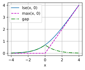
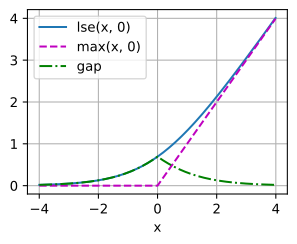
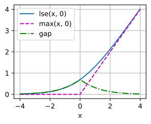
For two classes with logits \((x, 0)\) the loss’s first term is \(\mathrm{lse}(x, 0) = \log(1 + e^x)\), which approaches \(\max(x, 0)\) from above, with the gap largest at the tie \(x = 0\), where it equals \(\log 2 \approx 0.69\), our bound \(\log q\) for \(q = 2\):
x = d2l.arange(-4.0, 4.0, 0.01)
lse, mx = d2l.log(1 + d2l.exp(x)), (x + d2l.abs(x)) / 2
d2l.plot(x, [lse, mx, lse - mx], 'x', legend=['lse(x, 0)', 'max(x, 0)', 'gap'])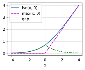
@d2l.add_to_class(d2l.Classifier)
def loss(self, Y_hat, Y, averaged=True):
    Y_hat = d2l.reshape(Y_hat, (-1, Y_hat.shape[-1]))
    Y = d2l.reshape(Y, (-1,))
    return F.cross_entropy(
Y_hat, Y, reduction='mean' if averaged else 'none')@d2l.add_to_class(d2l.Classifier)
def loss(self, Y_hat, Y, averaged=True):
Y_hat = d2l.reshape(Y_hat, (-1, Y_hat.shape[-1]))
Y = d2l.reshape(Y, (-1,))
reduction = (tf.keras.losses.Reduction.SUM_OVER_BATCH_SIZE
if averaged else tf.keras.losses.Reduction.NONE)
fn = tf.keras.losses.SparseCategoricalCrossentropy(
from_logits=True, reduction=reduction)
return fn(Y, Y_hat)@d2l.add_to_class(d2l.Classifier)
def loss(self, Y_hat, Y, averaged=True):
Y_hat = d2l.reshape(Y_hat, (-1, Y_hat.shape[-1]))
Y = d2l.reshape(Y, (-1,))
fn = optax.softmax_cross_entropy_with_integer_labels
return fn(Y_hat, Y).mean() if averaged else fn(Y_hat, Y)@d2l.add_to_class(d2l.Classifier)
def loss(self, Y_hat, Y, averaged=True):
Y_hat = d2l.reshape(Y_hat, (-1, Y_hat.shape[-1]))
Y = d2l.reshape(Y, (-1,))
fn = gluon.loss.SoftmaxCrossEntropyLoss()
l = fn(Y_hat, Y)
return l.mean() if averaged else lThe built-in fused loss (named differently in each library) takes logits, not probabilities: passing softmax outputs would apply the softmax twice. Correspondingly, the model’s forward returns raw logits and contains no softmax: the loss owns that step. We defined this loss on the base Classifier (note the #@save), so every classifier in the rest of the book inherits the numerically stable version.
3.5.3 Training
Next we train our model. We use Fashion-MNIST images, flattened to 784-dimensional feature vectors.
data = d2l.FashionMNIST(batch_size=256)
model = SoftmaxRegression(num_outputs=10, lr=0.1)
trainer = d2l.Trainer(max_epochs=10)
trainer.fit(model, data)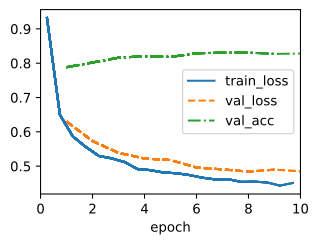
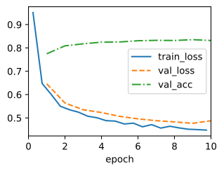
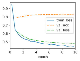
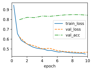
In the displayed run, training reaches about 83–84% validation accuracy, close to the from-scratch implementation in Section 3.4. The shorter program changes the implementation interface, not the underlying linear model.
3.5.4 Summary
The concise model uses a single linear layer for its logits and a framework cross-entropy operator for its loss. That operator combines log-softmax with negative log-likelihood, avoiding the overflow and underflow of an explicitly materialized softmax. The from-scratch version exposes the algebra and data flow; the concise version supplies the stable components normally used in applications. Comparing them makes clear which behavior belongs to the model and which belongs to its implementation.
3.5.5 Exercises
- Number formats. ● Deep learning uses several floating-point formats. Each consists of one sign bit, an exponent field and a mantissa field. The exponent and mantissa fields have 11 and 52 bits in FP64, 8 and 23 bits in FP32, 8 and 10 bits in TF32, 8 and 7 bits in BFLOAT16, and 5 and 10 bits in FP16. Assume that every format represents subnormal numbers as FP32 does. For each format, determine the smallest and largest argument of the exponential function for which the result neither underflows to \(0\) nor overflows. Present the result as a table with one row per format, and explain how each limit depends on the numbers of exponent and mantissa bits.
- [code] Double softmax. The
lossof this section expects logits. Suppose that a model’sforwardmistakenly ends with a softmax. The loss then receives a probability vector \(\mathbf{p}\) in place of the logits and evaluates \(-\log \mathrm{softmax}(\mathbf{p})_y\).- Find the smallest value this loss can take over all probability vectors \(\mathbf{p}\) and labels \(y\), as a function of the number of classes \(q\). Evaluate it for \(q = 10\).
- Copy the from-scratch
softmaxof Section 3.4, which is not part of thed2lpackage. SubclassSoftmaxRegressionso thatforwardapplies thissoftmaxto the logits. Train it withlr=0.1,d2l.FashionMNIST(batch_size=256), andd2l.Trainer(max_epochs=10). Compare its training loss and validation accuracy with those ofSoftmaxRegression, and relate the final training loss to the value from the previous step.
- [code] Fused loss on extreme logits. Section 3.4 showed that the from-scratch
softmaxreturnsNaNon the logits \(\mathbf{o} = (1000, 0, 0)\). Thatsoftmaxis not part of thed2lpackage, so copy it, and store \(\mathbf{o}\) as a \(1 \times 3\) matrix.- Pass \(\mathbf{o}\) to the
lossof this section, first with true class \(y = 0\) and then with \(y = 1\). Check both values against \(\ell(y, \mathbf{o}) = \log\sum_k \exp(o_k) - o_y\) evaluated by hand. - Compute the same two losses by the from-scratch route,
softmaxfollowed byd2l.cross_entropy. Explain each value it returns, and determine the largest finite loss this route can return. - Verify on benign logits such as \(\mathbf{o} = (2, 1, 0)\) that the two routes agree to floating-point precision.
- Pass \(\mathbf{o}\) to the
- [code] Log-sum-exp bound. Write \(\mathrm{lse}(\mathbf{o}) = \log\sum_k \exp(o_k)\) for logits \(\mathbf{o} \in \mathbb{R}^q\). By exercise 6 of Section 3.1, the gap \(\mathrm{lse}(\mathbf{o}) - \max_k o_k\) is at most \(\log q\).
- Show that the gap equals \(-\log \max_j \mathrm{softmax}(\mathbf{o})_j\).
- For each \(q \in \{2, 10, 100, 1000\}\), draw \(1000\) standard Gaussian logit vectors. Plot the mean gap against \(q\) together with the bound \(\log q\), and report the ratio of the two for each \(q\). How does this ratio change as \(q\) grows?