from d2l import torch as d2l
import torch
from torch import nn
from torch.nn import functional as F7.4 Residual Networks: ResNet, ResNeXt, and DenseNet
Adding layers should enlarge a model’s function class without making the shallower solution difficult to recover. Residual networks achieve this by parameterizing each block as a change to the identity map. We first formalize this inclusion of function classes and then implement residual blocks, ResNet, ResNeXt, and DenseNet.
import tensorflow as tf
from d2l import tensorflow as d2l
from d2l import jax as d2l
from flax import nnx
from jax import numpy as jnp
import jaxfrom d2l import mxnet as d2l
from mxnet import np, npx, init
from mxnet.gluon import nn
npx.set_np()7.4.1 Function Classes
Let \(\mathcal{F}\) be the class of functions represented by an architecture as its parameters vary. Given training data \((\mathbf{X},\mathbf{y})\), define the best empirical-loss value available in this class by
\[L^*_{\mathcal{F}} \stackrel{\textrm{def}}{=} \inf_{f\in\mathcal{F}} L(\mathbf{X},\mathbf{y},f). \tag{7.4.1}\]
If \(\mathcal{F}\subseteq\mathcal{F}'\), then \(L^*_{\mathcal{F}'}\leq L^*_{\mathcal{F}}\): the larger class can always reuse the best function available to the smaller one. This is a statement about representational capacity and the optimal training loss. It does not guarantee that an optimizer will find that function or that the resulting model will generalize better. For non-nested classes, even the empirical optima have no such ordering. Figure 7.4.1 illustrates containment rather than a distance to an undefined target function.
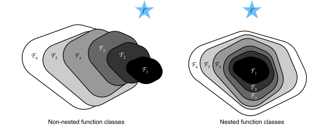
Thus, if larger function classes contain the smaller ones, increasing capacity cannot reduce expressive power. The containment may be equality, so the increase need not be strict. For deep neural networks, if a newly added block can represent the identity \(f(\mathbf{x}) = \mathbf{x}\), the deeper model contains the shallower one as a special case. This protects representation capacity; it does not guarantee that optimization will find the best member of the larger class.
ResNet (He et al. 2016) makes this containment easy to express: each added block can represent the identity mapping by setting its residual branch to zero. The resulting component is a residual block. With it, ResNet won the ImageNet Large Scale Visual Recognition Challenge in 2015. The design influenced how to build deep neural networks. For instance, residual blocks have been added to recurrent networks (Prakash et al. 2016; Kim et al. 2017). Likewise, Transformers (Vaswani et al. 2017) use them to stack many layers of networks efficiently. It is also used in graph neural networks (Kipf and Welling 2017) and, as a basic concept, it has been used extensively in computer vision (Redmon and Farhadi 2018; Ren et al. 2015). Highway networks (Srivastava et al. 2015) predate ResNet and share some of its motivation, using learned gates rather than a direct identity shortcut.
7.4.2 Residual Blocks
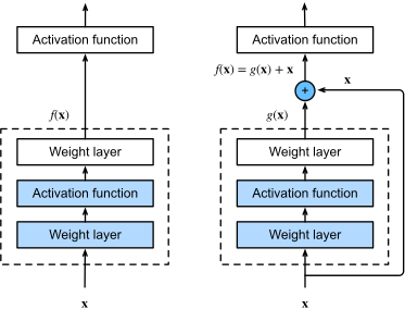
Consider the part of a neural network depicted in Figure 7.4.2. Denote the input by \(\mathbf{x}\). We assume that \(f(\mathbf{x})\), the desired underlying mapping we want to obtain by learning, is to be used as input to the activation function on the top. On the left, the portion within the dotted-line box must directly learn \(f(\mathbf{x})\). On the right, the portion within the dotted-line box needs to learn the residual mapping \(g(\mathbf{x}) = f(\mathbf{x}) - \mathbf{x}\), which is how the residual block derives its name. If the identity mapping \(f(\mathbf{x}) = \mathbf{x}\) is the desired underlying mapping, the residual mapping amounts to \(g(\mathbf{x}) = 0\) and it is thus easier to learn: we only need to push the weights and biases of the upper weight layer (e.g., fully connected layer and convolutional layer) within the dotted-line box to zero. The right figure illustrates the residual block of ResNet, where the solid line carrying the layer input \(\mathbf{x}\) to the addition operator is called a residual connection (or shortcut connection). Residual connections provide a direct path for activations and gradients through a stack of blocks. In fact, the residual block can be thought of as a special case of the multi-branch Inception block: it has two branches one of which is the identity mapping.
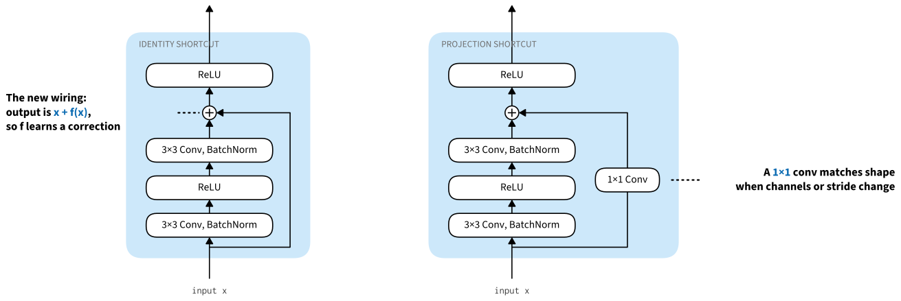
ResNet has VGG’s full \(3\times 3\) convolutional layer design. The residual block has two \(3\times 3\) convolutional layers with the same number of output channels. Each convolutional layer is followed by batch normalization, and the first is followed by a ReLU. We add the input to the second normalized output and then apply the final ReLU. Because that ReLU clips negative values, this post-activation block is exactly the identity only on inputs that are already nonnegative. The pre-activation variant discussed in the exercises places the activation inside the residual branch and permits an exact identity on arbitrary inputs. This kind of design requires that the output of the two convolutional layers has to be of the same shape as the input, so that they can be added together. If we want to change the number of channels, we need to introduce an additional \(1\times 1\) convolutional layer to transform the input into the desired shape for the addition operation. The code below implements both cases.
class Residual(nn.Module):
    """The Residual block of ResNet models."""
    def __init__(self, num_channels, use_1x1conv=False, strides=1):
        super().__init__()
        self.conv1 = nn.LazyConv2d(num_channels, kernel_size=3, padding=1,
                                   stride=strides)
        self.conv2 = nn.LazyConv2d(num_channels, kernel_size=3, padding=1)
        # Auto-enable 1x1 conv when downsampling so the residual shape matches.
        if use_1x1conv or strides != 1:
            self.conv3 = nn.LazyConv2d(num_channels, kernel_size=1,
                                       stride=strides)
        else:
            self.conv3 = None
        self.bn1 = nn.LazyBatchNorm2d()
        self.bn2 = nn.LazyBatchNorm2d()

    def forward(self, X):
        Y = F.relu(self.bn1(self.conv1(X)))
        Y = self.bn2(self.conv2(Y))
        if self.conv3:
            X = self.conv3(X)
        Y += X
        return F.relu(Y)
class Residual(tf.keras.Model):
"""The Residual block of ResNet models."""
def __init__(self, num_channels, use_1x1conv=False, strides=1):
super().__init__()
self.conv1 = tf.keras.layers.Conv2D(num_channels, padding='same',
kernel_size=3, strides=strides)
self.conv2 = tf.keras.layers.Conv2D(num_channels, kernel_size=3,
padding='same')
self.conv3 = None
# Auto-enable 1x1 conv when downsampling so the residual shape matches.
if use_1x1conv or strides != 1:
self.conv3 = tf.keras.layers.Conv2D(num_channels, kernel_size=1,
strides=strides)
self.bn1 = tf.keras.layers.BatchNormalization()
self.bn2 = tf.keras.layers.BatchNormalization()
def call(self, X):
Y = tf.keras.activations.relu(self.bn1(self.conv1(X)))
Y = self.bn2(self.conv2(Y))
if self.conv3 is not None:
X = self.conv3(X)
Y += X
return tf.keras.activations.relu(Y)class Residual(nnx.Module):
"""The Residual block of ResNet models."""
def __init__(self, num_channels, use_1x1conv=False, strides=(1, 1),
in_channels=None, rngs=None):
in_channels = num_channels if in_channels is None else in_channels
rngs = nnx.Rngs(d2l.get_key()) if rngs is None else rngs
self.conv1 = nnx.Conv(in_channels, num_channels, kernel_size=(3, 3),
padding='same', strides=strides, rngs=rngs)
self.conv2 = nnx.Conv(num_channels, num_channels, kernel_size=(3, 3),
padding='same', rngs=rngs)
# Auto-enable 1x1 conv when downsampling so the residual shape matches.
if use_1x1conv or any(s != 1 for s in strides):
self.conv3 = nnx.Conv(in_channels, num_channels,
kernel_size=(1, 1), strides=strides,
rngs=rngs)
else:
self.conv3 = None
self.bn1 = nnx.BatchNorm(num_channels, rngs=rngs)
self.bn2 = nnx.BatchNorm(num_channels, rngs=rngs)
def __call__(self, X):
Y = nnx.relu(self.bn1(self.conv1(X)))
Y = self.bn2(self.conv2(Y))
if self.conv3:
X = self.conv3(X)
Y += X
return nnx.relu(Y)class Residual(nn.Block):
"""The Residual block of ResNet models."""
def __init__(self, num_channels, use_1x1conv=False, strides=1):
super().__init__()
self.conv1 = nn.Conv2D(num_channels, kernel_size=3, padding=1,
strides=strides)
self.conv2 = nn.Conv2D(num_channels, kernel_size=3, padding=1)
# Auto-enable 1x1 conv when downsampling so the residual shape matches.
if use_1x1conv or strides != 1:
self.conv3 = nn.Conv2D(num_channels, kernel_size=1,
strides=strides)
else:
self.conv3 = None
self.bn1 = nn.BatchNorm()
self.bn2 = nn.BatchNorm()
def forward(self, X):
Y = npx.relu(self.bn1(self.conv1(X)))
Y = self.bn2(self.conv2(Y))
if self.conv3:
X = self.conv3(X)
return npx.relu(Y + X)This code generates two types of networks: one where we add the input directly to the output before applying the ReLU nonlinearity whenever use_1x1conv=False and the stride is 1; and one where we adjust channels and resolution by means of a \(1 \times 1\) convolution before adding, which the block enables automatically whenever use_1x1conv=True or the stride is not 1. Figure 7.4.3 illustrates this.
We first consider matching input and output shapes, for which the \(1 \times 1\) convolution is unnecessary.
blk = Residual(3)
X = d2l.randn(4, 3, 6, 6)
blk(X).shape
torch.Size([4, 3, 6, 6])blk = Residual(3)
X = d2l.normal((4, 6, 6, 3))
Y = blk(X)
Y.shapeTensorShape([4, 6, 6, 3])blk = Residual(3)
X = jax.random.normal(d2l.get_key(), (4, 6, 6, 3))
blk(X).shape(4, 6, 6, 3)blk = Residual(3)
blk.initialize()
X = d2l.randn(4, 3, 6, 6)
blk(X).shape(4, 3, 6, 6)We also have the option to halve the output height and width while increasing the number of output channels. In this case we use \(1 \times 1\) convolutions via use_1x1conv=True. This comes in handy at the beginning of each ResNet block to reduce the spatial dimensionality via strides=2.
blk = Residual(6, use_1x1conv=True, strides=2)
blk(X).shape
torch.Size([4, 6, 3, 3])blk = Residual(6, use_1x1conv=True, strides=2)
blk(X).shapeTensorShape([4, 3, 3, 6])blk = Residual(6, use_1x1conv=True, strides=(2, 2), in_channels=3)
blk(X).shape(4, 3, 3, 6)blk = Residual(6, use_1x1conv=True, strides=2)
blk.initialize()
blk(X).shape(4, 6, 3, 3)7.4.3 ResNet Model
The first two layers of ResNet are the same as those of the GoogLeNet we described before: the \(7\times 7\) convolutional layer with 64 output channels and a stride of 2 is followed by the \(3\times 3\) max-pooling layer with a stride of 2. The difference is the batch normalization layer added after each convolutional layer in ResNet.
class ResNet(d2l.Classifier):
    def b1(self):
        return nn.Sequential(
            nn.LazyConv2d(64, kernel_size=7, stride=2, padding=3),
            nn.LazyBatchNorm2d(), nn.ReLU(),
            nn.MaxPool2d(kernel_size=3, stride=2, padding=1))
class ResNet(d2l.Classifier):
def b1(self):
return tf.keras.models.Sequential([
tf.keras.layers.Conv2D(64, kernel_size=7, strides=2,
padding='same'),
tf.keras.layers.BatchNormalization(),
tf.keras.layers.Activation('relu'),
tf.keras.layers.MaxPool2D(pool_size=3, strides=2,
padding='same')])class ResNet(d2l.Classifier):
def __init__(self, arch, lr=0.1, num_classes=10, in_channels=1, rngs=None):
super().__init__()
self.save_hyperparameters(ignore=['rngs'])
rngs = nnx.Rngs(d2l.get_key()) if rngs is None else rngs
self.net = self.create_net(in_channels, rngs)
def b1(self, in_channels, rngs):
return nnx.Sequential(
nnx.Conv(in_channels, 64, kernel_size=(7, 7), strides=(2, 2),
padding='same', rngs=rngs),
nnx.BatchNorm(64, rngs=rngs), nnx.relu,
lambda x: nnx.max_pool(x, window_shape=(3, 3), strides=(2, 2),
padding='same'))class ResNet(d2l.Classifier):
def b1(self):
net = nn.Sequential()
net.add(nn.Conv2D(64, kernel_size=7, strides=2, padding=3),
nn.BatchNorm(), nn.Activation('relu'),
nn.MaxPool2D(pool_size=3, strides=2, padding=1))
return netGoogLeNet uses four modules made up of Inception blocks. However, ResNet uses four modules made up of residual blocks, each of which uses several residual blocks with the same number of output channels. The number of channels in the first module is the same as the number of input channels. Since a max-pooling layer with a stride of 2 has already been used, it is not necessary to reduce the height and width. In the first residual block for each of the subsequent modules, the number of channels is doubled compared with that of the previous module, and the height and width are halved.
@d2l.add_to_class(ResNet)
def block(self, num_residuals, num_channels, first_block=False):
    blk = []
    for i in range(num_residuals):
        if i == 0 and not first_block:
            blk.append(Residual(num_channels, use_1x1conv=True, strides=2))
        else:
            blk.append(Residual(num_channels))
return nn.Sequential(*blk)@d2l.add_to_class(ResNet)
def block(self, num_residuals, num_channels, first_block=False):
blk = tf.keras.models.Sequential()
for i in range(num_residuals):
if i == 0 and not first_block:
blk.add(Residual(num_channels, use_1x1conv=True, strides=2))
else:
blk.add(Residual(num_channels))
return blk@d2l.add_to_class(ResNet)
def block(self, num_residuals, num_channels, in_channels,
first_block=False, rngs=None):
blk = []
for i in range(num_residuals):
if i == 0 and not first_block:
blk.append(Residual(num_channels, use_1x1conv=True,
strides=(2, 2), in_channels=in_channels,
rngs=rngs))
else:
blk.append(Residual(num_channels, in_channels=in_channels,
rngs=rngs))
in_channels = num_channels
return nnx.Sequential(*blk)@d2l.add_to_class(ResNet)
def block(self, num_residuals, num_channels, first_block=False):
blk = nn.Sequential()
for i in range(num_residuals):
if i == 0 and not first_block:
blk.add(Residual(num_channels, use_1x1conv=True, strides=2))
else:
blk.add(Residual(num_channels))
return blkWe assemble the modules into ResNet, using two residual blocks per module. As in GoogLeNet, global average pooling precedes the fully connected output layer.
@d2l.add_to_class(ResNet)
def __init__(self, arch, lr=0.1, num_classes=10):
    super(ResNet, self).__init__()
    self.save_hyperparameters()
    self.net = nn.Sequential(self.b1())
    for i, b in enumerate(arch):
        self.net.add_module(f'b{i+2}', self.block(*b, first_block=(i==0)))
    self.net.add_module('last', nn.Sequential(
        nn.AdaptiveAvgPool2d((1, 1)), nn.Flatten(),
        nn.LazyLinear(num_classes)))
self.net.apply(d2l.init_cnn)@d2l.add_to_class(ResNet)
def __init__(self, arch, lr=0.1, num_classes=10):
super(ResNet, self).__init__()
self.save_hyperparameters()
self.net = self.b1()
for i, b in enumerate(arch):
self.net.add(self.block(*b, first_block=(i==0)))
self.net.add(tf.keras.models.Sequential([
tf.keras.layers.GlobalAvgPool2D(),
tf.keras.layers.Dense(units=num_classes)]))@d2l.add_to_class(ResNet)
def create_net(self, in_channels, rngs):
layers = [self.b1(in_channels, rngs)]
stage_channels = 64
for i, (num_residuals, num_channels) in enumerate(self.arch):
layers.append(self.block(num_residuals, num_channels, stage_channels,
first_block=(i == 0), rngs=rngs))
stage_channels = num_channels
layers.append(nnx.Sequential(
lambda x: x.mean(axis=(1, 2)), # global avg pooling over H, W (NHWC)
nnx.Linear(stage_channels, self.num_classes, rngs=rngs)))
return nnx.Sequential(*layers)@d2l.add_to_class(ResNet)
def __init__(self, arch, lr=0.1, num_classes=10):
super(ResNet, self).__init__()
self.save_hyperparameters()
self.net = nn.Sequential()
self.net.add(self.b1())
for i, b in enumerate(arch):
self.net.add(self.block(*b, first_block=(i==0)))
self.net.add(nn.GlobalAvgPool2D(), nn.Dense(num_classes))
self.net.initialize(init.Xavier())There are four convolutional layers in each module (excluding the \(1\times 1\) convolutional layer). Together with the first \(7\times 7\) convolutional layer and the final fully connected layer, there are 18 layers in total. Therefore, this model is commonly known as ResNet-18. By configuring different numbers of channels and residual blocks in the module, we can create different ResNet models, such as the deeper 152-layer ResNet-152. Although the main architecture of ResNet is similar to that of GoogLeNet, ResNet’s structure is simpler and easier to modify. All these factors have resulted in the rapid and widespread use of ResNet. Figure 7.4.4 depicts the full ResNet-18.
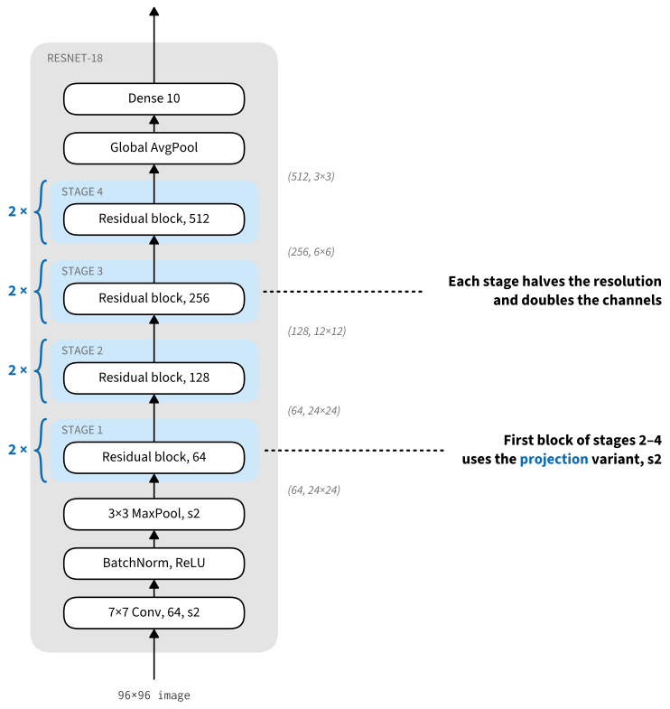
Before training ResNet, let’s observe how the input shape changes across different modules in ResNet. As in all the previous architectures, the resolution decreases while the number of channels increases up until the point where a global average pooling layer aggregates all features.
class ResNet18(ResNet):
    def __init__(self, lr=0.1, num_classes=10):
        super().__init__(((2, 64), (2, 128), (2, 256), (2, 512)),
                       lr, num_classes)
class ResNet18(ResNet):
def __init__(self, lr=0.1, num_classes=10):
super().__init__(((2, 64), (2, 128), (2, 256), (2, 512)),
lr, num_classes)class ResNet18(ResNet):
def __init__(self, lr=0.1, num_classes=10, in_channels=1, rngs=None):
super().__init__(((2, 64), (2, 128), (2, 256), (2, 512)),
lr, num_classes, in_channels, rngs)class ResNet18(ResNet):
def __init__(self, lr=0.1, num_classes=10):
super().__init__(((2, 64), (2, 128), (2, 256), (2, 512)),
lr, num_classes)ResNet18().layer_summary((1, 1, 96, 96))Sequential output shape: torch.Size([1, 64, 24, 24])
Sequential output shape: torch.Size([1, 64, 24, 24])
Sequential output shape: torch.Size([1, 128, 12, 12])
Sequential output shape: torch.Size([1, 256, 6, 6])
Sequential output shape: torch.Size([1, 512, 3, 3])
Sequential output shape: torch.Size([1, 10])ResNet18().layer_summary((1, 96, 96, 1))Conv2D output shape: (1, 48, 48, 64)
BatchNormalization output shape: (1, 48, 48, 64)
Activation output shape: (1, 48, 48, 64)
MaxPooling2D output shape: (1, 24, 24, 64)
Sequential output shape: (1, 24, 24, 64)
Sequential output shape: (1, 12, 12, 128)
Sequential output shape: (1, 6, 6, 256)
Sequential output shape: (1, 3, 3, 512)
Sequential output shape: (1, 10)ResNet18().layer_summary((1, 96, 96, 1))Sequential output shape: (1, 24, 24, 64)
Sequential output shape: (1, 24, 24, 64)
Sequential output shape: (1, 12, 12, 128)
Sequential output shape: (1, 6, 6, 256)
Sequential output shape: (1, 3, 3, 512)
Sequential output shape: (1, 10)ResNet18().layer_summary((1, 1, 96, 96))Sequential output shape: (1, 64, 24, 24)
Sequential output shape: (1, 64, 24, 24)
Sequential output shape: (1, 128, 12, 12)
Sequential output shape: (1, 256, 6, 6)
Sequential output shape: (1, 512, 3, 3)
GlobalAvgPool2D output shape: (1, 512, 1, 1)
Dense output shape: (1, 10)7.4.4 Training
We train ResNet on Fashion-MNIST under the same protocol as the preceding models. In this run the training loss falls below the validation loss, which indicates a generalization gap. Additional data, stronger augmentation, regularization, and a smaller model are distinct possible responses; this single curve does not identify which would help most.
model = ResNet18(lr=0.01)
trainer = d2l.Trainer(max_epochs=10, num_gpus=1)
data = d2l.FashionMNIST(batch_size=128, resize=(96, 96))
model.apply_init([next(iter(data.get_dataloader(True)))[0]], d2l.init_cnn)
trainer.fit(model, data)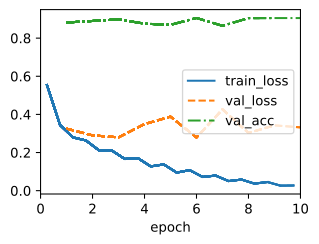
trainer = d2l.Trainer(max_epochs=10)
data = d2l.FashionMNIST(batch_size=128, resize=(96, 96))
with d2l.try_gpu():
    model = ResNet18(lr=0.01)
    trainer.fit(model, data)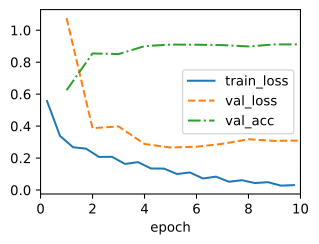
model = ResNet18(lr=0.01)
trainer = d2l.Trainer(max_epochs=10, num_gpus=1)
data = d2l.FashionMNIST(batch_size=128, resize=(96, 96))
trainer.fit(model, data)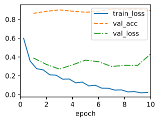
model = ResNet18(lr=0.01)
trainer = d2l.Trainer(max_epochs=10, num_gpus=1)
data = d2l.FashionMNIST(batch_size=128, resize=(96, 96))
trainer.fit(model, data)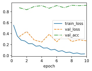
7.4.5 ResNeXt
One of the challenges one encounters in the design of ResNet is the trade-off between nonlinearity and dimensionality within a given block. That is, we could add more nonlinearity by increasing the number of layers, or by increasing the width of the convolutions. An alternative strategy is to increase the number of channels that can carry information between blocks. Unfortunately, the latter comes with a quadratic penalty since the computational cost of ingesting \(c_\textrm{i}\) channels and emitting \(c_\textrm{o}\) channels is proportional to \(\mathcal{O}(c_\textrm{i} \cdot c_\textrm{o})\) (see our discussion in Section 6.4).
We can take some inspiration from the Inception block of Figure 7.2.3 which has information flowing through the block in separate groups. Applying the idea of multiple independent groups to the ResNet block of Figure 7.4.3 led to the design of ResNeXt (Xie et al. 2017). Different from the smorgasbord of transformations in Inception, ResNeXt adopts the same transformation in all branches, thus minimizing the need for manual tuning of each branch.
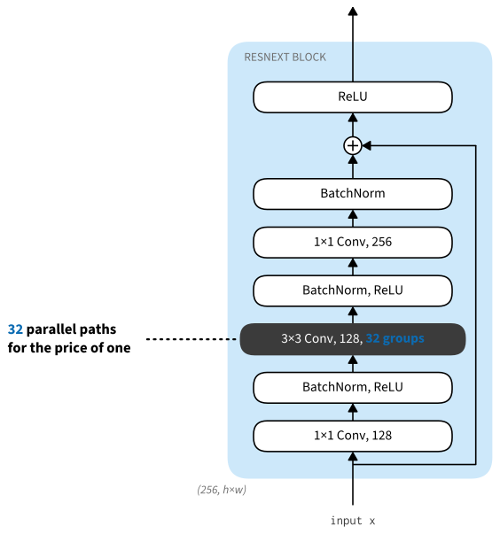
Breaking up a convolution from \(c_\textrm{i}\) to \(c_\textrm{o}\) channels into one of \(g\) groups of size \(c_\textrm{i}/g\) generating \(g\) outputs of size \(c_\textrm{o}/g\) is called, quite fittingly, a grouped convolution. The arithmetic cost is reduced from \(\mathcal{O}(c_\textrm{i} \cdot c_\textrm{o})\) to \(\mathcal{O}(g \cdot (c_\textrm{i}/g) \cdot (c_\textrm{o}/g)) = \mathcal{O}(c_\textrm{i} \cdot c_\textrm{o} / g)\), i.e., it uses \(g\) times fewer multiply-adds. The number of parameters is likewise reduced from a \(c_\textrm{i} \times c_\textrm{o}\) matrix to \(g\) smaller matrices of size \((c_\textrm{i}/g) \times (c_\textrm{o}/g)\). Wall-clock speedup depends on kernel efficiency and memory traffic and can be much smaller. In what follows we assume that both \(c_\textrm{i}\) and \(c_\textrm{o}\) are divisible by \(g\).
The only challenge in this design is that no information is exchanged between the \(g\) groups. The ResNeXt block of Figure 7.4.5 amends this in two ways: the grouped convolution with a \(3 \times 3\) kernel is sandwiched in between two \(1 \times 1\) convolutions. The second one serves double duty in changing the number of channels back. The benefit is that we only pay the \(\mathcal{O}(c \cdot b)\) cost for \(1 \times 1\) kernels and can make do with an \(\mathcal{O}(b^2 / g)\) cost for \(3 \times 3\) kernels. Similar to the residual block implementation in Section 7.4.2, the residual connection is replaced (thus generalized) by a \(1 \times 1\) convolution.
The block in Figure 7.4.5 will also play a major role in the design of generic modern CNNs in Section 7.8. Grouped convolutions appeared in AlexNet (Krizhevsky et al. 2012), where most channels were split into two groups so that each GPU could process one group with limited cross-GPU communication.
The following implementation of the ResNeXtBlock class takes as argument groups (\(g\)), with bot_channels (\(b\)) intermediate (bottleneck) channels. Lastly, when we need to reduce the height and width of the representation, we add a stride of \(2\) by setting use_1x1conv=True, strides=2.
class ResNeXtBlock(nn.Module):
    """The ResNeXt block."""
    def __init__(self, num_channels, groups, bot_mul, use_1x1conv=False,
                 strides=1):
        super().__init__()
        bot_channels = int(round(num_channels * bot_mul))
        self.conv1 = nn.LazyConv2d(bot_channels, kernel_size=1, stride=1)
        self.conv2 = nn.LazyConv2d(bot_channels, kernel_size=3,
                                   stride=strides, padding=1,
                                   groups=groups)
        self.conv3 = nn.LazyConv2d(num_channels, kernel_size=1, stride=1)
        self.bn1 = nn.LazyBatchNorm2d()
        self.bn2 = nn.LazyBatchNorm2d()
        self.bn3 = nn.LazyBatchNorm2d()
        if use_1x1conv:
            self.conv4 = nn.LazyConv2d(num_channels, kernel_size=1,
                                       stride=strides)
            self.bn4 = nn.LazyBatchNorm2d()
        else:
            self.conv4 = None

    def forward(self, X):
        Y = F.relu(self.bn1(self.conv1(X)))
        Y = F.relu(self.bn2(self.conv2(Y)))
        Y = self.bn3(self.conv3(Y))
        if self.conv4:
            X = self.bn4(self.conv4(X))
        return F.relu(Y + X)
class ResNeXtBlock(tf.keras.Model):
"""The ResNeXt block."""
def __init__(self, num_channels, groups, bot_mul, use_1x1conv=False,
strides=1):
super().__init__()
bot_channels = int(round(num_channels * bot_mul))
self.conv1 = tf.keras.layers.Conv2D(bot_channels, 1, strides=1)
self.conv2 = tf.keras.layers.Conv2D(bot_channels, 3, strides=strides,
padding="same",
groups=groups)
self.conv3 = tf.keras.layers.Conv2D(num_channels, 1, strides=1)
self.bn1 = tf.keras.layers.BatchNormalization()
self.bn2 = tf.keras.layers.BatchNormalization()
self.bn3 = tf.keras.layers.BatchNormalization()
if use_1x1conv:
self.conv4 = tf.keras.layers.Conv2D(num_channels, 1,
strides=strides)
self.bn4 = tf.keras.layers.BatchNormalization()
else:
self.conv4 = None
def call(self, X):
Y = tf.keras.activations.relu(self.bn1(self.conv1(X)))
Y = tf.keras.activations.relu(self.bn2(self.conv2(Y)))
Y = self.bn3(self.conv3(Y))
if self.conv4:
X = self.bn4(self.conv4(X))
return tf.keras.activations.relu(Y + X)class ResNeXtBlock(nnx.Module):
"""The ResNeXt block."""
def __init__(self, num_channels, groups, bot_mul, use_1x1conv=False,
strides=(1, 1), in_channels=None, rngs=None):
in_channels = num_channels if in_channels is None else in_channels
rngs = nnx.Rngs(d2l.get_key()) if rngs is None else rngs
bot_channels = int(round(num_channels * bot_mul))
self.conv1 = nnx.Conv(in_channels, bot_channels, kernel_size=(1, 1),
strides=(1, 1), rngs=rngs)
self.conv2 = nnx.Conv(bot_channels, bot_channels,
kernel_size=(3, 3), strides=strides,
padding='same', feature_group_count=groups,
rngs=rngs)
self.conv3 = nnx.Conv(bot_channels, num_channels,
kernel_size=(1, 1), strides=(1, 1), rngs=rngs)
self.bn1 = nnx.BatchNorm(bot_channels, rngs=rngs)
self.bn2 = nnx.BatchNorm(bot_channels, rngs=rngs)
self.bn3 = nnx.BatchNorm(num_channels, rngs=rngs)
if use_1x1conv:
self.conv4 = nnx.Conv(in_channels, num_channels,
kernel_size=(1, 1), strides=strides,
rngs=rngs)
self.bn4 = nnx.BatchNorm(num_channels, rngs=rngs)
else:
self.conv4 = None
def __call__(self, X):
Y = nnx.relu(self.bn1(self.conv1(X)))
Y = nnx.relu(self.bn2(self.conv2(Y)))
Y = self.bn3(self.conv3(Y))
if self.conv4:
X = self.bn4(self.conv4(X))
return nnx.relu(Y + X)class ResNeXtBlock(nn.Block):
"""The ResNeXt block."""
def __init__(self, num_channels, groups, bot_mul,
use_1x1conv=False, strides=1):
super().__init__()
bot_channels = int(round(num_channels * bot_mul))
self.conv1 = nn.Conv2D(bot_channels, kernel_size=1, padding=0,
strides=1)
self.conv2 = nn.Conv2D(bot_channels, kernel_size=3, padding=1,
strides=strides, groups=groups)
self.conv3 = nn.Conv2D(num_channels, kernel_size=1, padding=0,
strides=1)
self.bn1 = nn.BatchNorm()
self.bn2 = nn.BatchNorm()
self.bn3 = nn.BatchNorm()
if use_1x1conv:
self.conv4 = nn.Conv2D(num_channels, kernel_size=1,
strides=strides)
self.bn4 = nn.BatchNorm()
else:
self.conv4 = None
def forward(self, X):
Y = npx.relu(self.bn1(self.conv1(X)))
Y = npx.relu(self.bn2(self.conv2(Y)))
Y = self.bn3(self.conv3(Y))
if self.conv4:
X = self.bn4(self.conv4(X))
return npx.relu(Y + X)Its use is entirely analogous to that of the ResNetBlock discussed previously. For instance, when using (use_1x1conv=False, strides=1), the input and output are of the same shape. Alternatively, setting use_1x1conv=True, strides=2 halves the output height and width.
blk = ResNeXtBlock(32, 16, 1)
X = d2l.randn(4, 32, 96, 96)
blk(X).shape
torch.Size([4, 32, 96, 96])blk = ResNeXtBlock(32, 16, 1)
X = d2l.normal((4, 96, 96, 32))
Y = blk(X)
Y.shapeTensorShape([4, 96, 96, 32])blk = ResNeXtBlock(32, 16, 1)
X = jnp.zeros((4, 96, 96, 32))
blk(X).shape(4, 96, 96, 32)blk = ResNeXtBlock(32, 16, 1)
blk.initialize()
X = d2l.randn(4, 32, 96, 96)
blk(X).shape(4, 32, 96, 96)7.4.6 Concatenation instead of Addition: DenseNet
The residual block computes \(f(\mathbf{x}) = \mathbf{x} + g(\mathbf{x})\), splitting a function into the identity plus a correction, much as a Taylor expansion splits a function into a leading term plus higher-order refinements. What if we want to keep more than two terms, without forcing them to share a sum? DenseNet (dense convolutional network) (Huang et al. 2017) answers by concatenating a layer’s output onto its input along the channel dimension, so every layer receives the feature maps of all layers that precede it. Applying an increasingly complex sequence of functions thus maps \(\mathbf{x}\) to
\[ \mathbf{x} \to \left[ \mathbf{x}, f_1(\mathbf{x}), f_2\left(\left[\mathbf{x}, f_1\left(\mathbf{x}\right)\right]\right), f_3\left(\left[\mathbf{x}, f_1\left(\mathbf{x}\right), f_2\left(\left[\mathbf{x}, f_1\left(\mathbf{x}\right)\right]\right)\right]\right), \ldots\right], \]
where \([\cdot, \cdot]\) denotes concatenation. The name reflects the resulting dependency graph: the last layer of such a chain is densely connected to all its predecessors. Figure 7.4.6 contrasts the two designs.
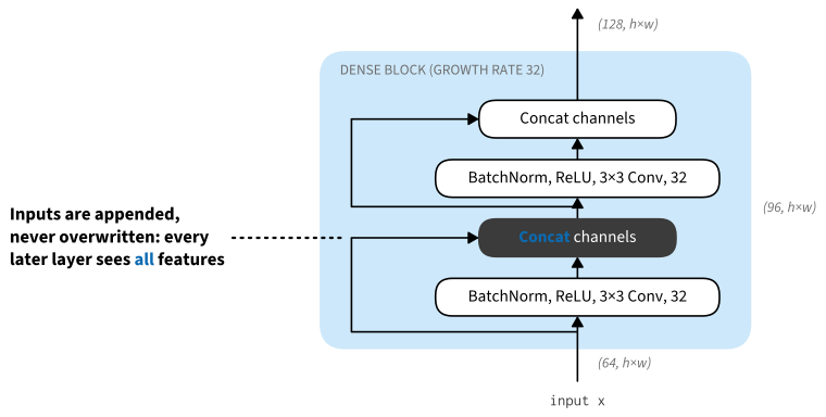
A DenseNet consists of dense blocks, which define how outputs are concatenated, alternating with transition layers, which shrink the accumulated channels back down. Each convolution inside a dense block uses the “batch normalization, activation, and convolution” pre-activation ordering explored in the exercises below.
def conv_block(num_channels):
    return nn.Sequential(
        nn.LazyBatchNorm2d(), nn.ReLU(),
        nn.LazyConv2d(num_channels, kernel_size=3, padding=1))
class ConvBlock(tf.keras.layers.Layer):
def __init__(self, num_channels):
super(ConvBlock, self).__init__()
self.bn = tf.keras.layers.BatchNormalization()
self.relu = tf.keras.layers.ReLU()
self.conv = tf.keras.layers.Conv2D(
filters=num_channels, kernel_size=(3, 3), padding='same')
self.listLayers = [self.bn, self.relu, self.conv]
def call(self, x):
y = x
for layer in self.listLayers:
y = layer(y)
return yclass ConvBlock(nnx.Module):
def __init__(self, in_channels, num_channels, rngs):
self.bn = nnx.BatchNorm(in_channels, rngs=rngs)
self.conv = nnx.Conv(in_channels, num_channels, kernel_size=(3, 3),
padding=(1, 1), rngs=rngs)
def __call__(self, X):
return self.conv(nnx.relu(self.bn(X)))def conv_block(num_channels):
blk = nn.Sequential()
blk.add(nn.BatchNorm(),
nn.Activation('relu'),
nn.Conv2D(num_channels, kernel_size=3, padding=1))
return blkA dense block consists of multiple convolution blocks, each using the same number of output channels. In the forward propagation, however, we concatenate the input and output of each convolution block on the channel dimension. Lazy evaluation allows us to adjust the dimensionality automatically.
class DenseBlock(nn.Module):
    def __init__(self, num_convs, num_channels):
        super(DenseBlock, self).__init__()
        layer = []
        for i in range(num_convs):
            layer.append(conv_block(num_channels))
        self.net = nn.Sequential(*layer)

    def forward(self, X):
        for blk in self.net:
            Y = blk(X)
            # Concatenate input and output of each block along the channels
            X = torch.cat((X, Y), dim=1)
        return X
class DenseBlock(tf.keras.layers.Layer):
def __init__(self, num_convs, num_channels):
super(DenseBlock, self).__init__()
self.listLayers = []
for _ in range(num_convs):
self.listLayers.append(ConvBlock(num_channels))
def call(self, x):
for layer in self.listLayers:
y = layer(x)
# Concatenate input and output of each block along the channels
x = tf.keras.layers.concatenate([x, y], axis=-1)
return xclass DenseBlock(nnx.Module):
def __init__(self, num_convs, num_channels, in_channels=3, rngs=None):
rngs = nnx.Rngs(d2l.get_key()) if rngs is None else rngs
layers = []
for i in range(num_convs):
layers.append(ConvBlock(
in_channels + i * num_channels, num_channels, rngs))
self.layers = nnx.List(layers)
def __call__(self, X):
for layer in self.layers:
Y = layer(X)
# Concatenate input and output of each block along the channels
X = jnp.concatenate((X, Y), axis=-1)
return Xclass DenseBlock(nn.Block):
def __init__(self, num_convs, num_channels):
super().__init__()
self.net = nn.Sequential()
for _ in range(num_convs):
self.net.add(conv_block(num_channels))
def forward(self, X):
for blk in self.net:
Y = blk(X)
# Concatenate input and output of each block along the channels
X = np.concatenate((X, Y), axis=1)
return XIn the following example, we define a DenseBlock instance with two convolution blocks of 10 output channels. When using an input with three channels, we will get an output with \(3 + 10 + 10=23\) channels. The number of convolution block channels controls the growth in the number of output channels relative to the number of input channels. This is also referred to as the growth rate.
blk = DenseBlock(2, 10)
X = torch.randn(4, 3, 8, 8)
Y = blk(X)
Y.shape
torch.Size([4, 23, 8, 8])blk = DenseBlock(2, 10)
X = tf.random.uniform((4, 8, 8, 3))
Y = blk(X)
Y.shapeTensorShape([4, 8, 8, 23])blk = DenseBlock(2, 10)
X = jnp.zeros((4, 8, 8, 3))
Y = blk(X)
Y.shape(4, 8, 8, 23)blk = DenseBlock(2, 10)
X = np.random.uniform(size=(4, 3, 8, 8))
blk.initialize()
Y = blk(X)
Y.shape(4, 23, 8, 8)Since each dense block increases the number of channels, stacking many of them without correction would produce an excessively wide model. A transition layer reduces the number of channels by a \(1\times 1\) convolution and halves the height and width via average pooling with a stride of 2.
def transition_block(num_channels):
    return nn.Sequential(
        nn.LazyBatchNorm2d(), nn.ReLU(),
        nn.LazyConv2d(num_channels, kernel_size=1),
        nn.AvgPool2d(kernel_size=2, stride=2))
class TransitionBlock(tf.keras.layers.Layer):
def __init__(self, num_channels, **kwargs):
super(TransitionBlock, self).__init__(**kwargs)
self.batch_norm = tf.keras.layers.BatchNormalization()
self.relu = tf.keras.layers.ReLU()
self.conv = tf.keras.layers.Conv2D(num_channels, kernel_size=1)
self.avg_pool = tf.keras.layers.AvgPool2D(pool_size=2, strides=2)
def call(self, x):
x = self.batch_norm(x)
x = self.relu(x)
x = self.conv(x)
return self.avg_pool(x)class TransitionBlock(nnx.Module):
def __init__(self, in_channels, num_channels, rngs=None):
rngs = nnx.Rngs(d2l.get_key()) if rngs is None else rngs
self.bn = nnx.BatchNorm(in_channels, rngs=rngs)
self.conv = nnx.Conv(in_channels, num_channels,
kernel_size=(1, 1), rngs=rngs)
def __call__(self, X):
X = self.conv(nnx.relu(self.bn(X)))
X = nnx.avg_pool(X, window_shape=(2, 2), strides=(2, 2))
return Xdef transition_block(num_channels):
blk = nn.Sequential()
blk.add(nn.BatchNorm(), nn.Activation('relu'),
nn.Conv2D(num_channels, kernel_size=1),
nn.AvgPool2D(pool_size=2, strides=2))
return blkApply a transition layer with 10 channels to the output of the dense block in the previous example. This reduces the number of output channels to 10, and halves the height and width.
blk = transition_block(10)
blk(Y).shape
torch.Size([4, 10, 4, 4])blk = TransitionBlock(10)
blk(Y).shapeTensorShape([4, 4, 4, 10])blk = TransitionBlock(23, 10)
blk(Y).shape(4, 4, 4, 10)blk = transition_block(10)
blk.initialize()
blk(Y).shape(4, 10, 4, 4)A full DenseNet alternates four dense blocks with transition layers, mirroring the four-stage layout of ResNet-18; assembling and training one is a straightforward variation on the ResNet code above. Feature reuse makes DenseNet parameter-efficient: it reached ResNet-level ImageNet accuracy with fewer parameters. Concatenation nevertheless carries a cost that addition does not. The unique feature maps grow linearly with depth, but a naive implementation repeatedly materializes ever-wider concatenations and temporary normalized outputs, producing quadratic memory growth inside a dense block. Memory-efficient implementations recompute those temporaries during backpropagation (Pleiss et al. 2017). The remaining activation traffic helped residual addition become the more common choice at scale.
7.4.7 Summary and Discussion
Nested function classes are desirable because adding capacity then preserves the functions already available. A residual branch parametrizes a block as the identity plus a correction. In a pre-activation block, setting that correction to zero gives the identity exactly; in the post-activation block used above, the statement holds on the nonnegative inputs produced by the preceding ReLU.
The residual mapping makes a near-identity transformation accessible by driving the correction toward zero, while the shortcut supplies a direct path for activations and gradients. This enabled the original ResNet experiments to train networks as deep as 152 layers (He et al. 2016). Residual branches can also be initialized near the identity, for example by zero-initializing the final normalization scale. Ordinary randomly initialized residual blocks are not exact identities, and inserting new blocks during training requires a separate function-preserving procedure.
Prior to residual connections, bypassing paths with gating units were introduced to effectively train highway networks with over 100 layers (Srivastava et al. 2015). Using identity functions as bypassing paths, ResNet performed well on multiple computer vision tasks. Residual connections had a major influence on the design of subsequent deep neural networks, of either convolutional or sequential nature. As we will introduce later, the Transformer architecture (Vaswani et al. 2017) adopts residual connections (together with other design choices) and is pervasive in areas as diverse as language, vision, speech, and reinforcement learning. Every transformer block in a large language model, and every block of the denoising networks behind diffusion models, is a residual block. By parameter count, most residual blocks in the world now live outside convolutional networks.
ResNeXt illustrates the trade between arithmetic and activation width. A grouped convolution is a block-diagonal channel-mixing matrix, reducing multiply-adds while retaining a wide representation. ShiftNet (Wu et al. 2018) takes this idea further by replacing spatial multiplications with shifts of channel activations. The shifts use no floating-point multiply-adds, though moving the activation data still incurs memory traffic.
A common feature of the designs we have discussed so far is that the network design is fairly manual, primarily relying on the ingenuity of the designer to find the “right” network hyperparameters. While clearly feasible, it is also very costly in terms of human time and there is no guarantee that the outcome is optimal in any sense. In Section 7.8 we will discuss a number of strategies for obtaining high quality networks in a more automated fashion. In particular, we will review the notion of network design spaces that led to the RegNetX/Y models (Radosavovic et al. 2020).
7.4.8 Exercises
- Inception versus residual blocks. In the
archof GoogLeNet (Section 7.2.3), the second block of the middle group has branch widths \(c_1 = 160\), \(c_2 = (112, 224)\), \(c_3 = (24, 64)\), and \(c_4 = 64\), and it maps 512 input channels to 512 output channels. Compare it with a 512-channelResidualblock that uses an identity shortcut.- Count the convolution weights and the multiply-adds per output pixel of both blocks, ignoring biases and normalization parameters.
- A
Residualblock whose residual branch outputs zero is the identity on nonnegative inputs. Determine whether any choice of parameters makes the Inception block the identity on nonnegative inputs, and state what the answer implies for deepening GoogLeNet by inserting Inception blocks.
- [code] ResNet variants. ● Table 1 of He et al. (2016) specifies ResNet-18 to ResNet-152 by the number of blocks per stage and by the block type.
- Build ResNet-34 by passing its block counts as
archtoResNetand report its parameter count againstResNet18. - ResNet-50 and its deeper relatives use a bottleneck block: a \(1 \times 1\) convolution that reduces the width fourfold, a \(3 \times 3\) convolution, and a \(1 \times 1\) convolution that restores the width.
ResNeXtBlockwithgroups=1andbot_mul=0.25implements this block. Compare its parameter count and multiply-adds with those ofResidualat the same input and output width, and with those ofResidualat a quarter of that width, which is the width of the matching ResNet-34 stage. - Override
blockin a subclass ofResNetso that it stacks bottleneck blocks, build ResNet-50, and compare its parameter count with ResNet-34’s.
- Build ResNet-34 by passing its block counts as
- Pre-activation ordering. He et al. (2016)*1 moved batch normalization and the ReLU in front of each convolution of the residual branch and removed the ReLU after the addition (their Figure 1), so that a block computes \(\mathbf{x} + g(\mathbf{x})\) with the identity path left untouched. The DenseNet convolution block in Section 7.4.6 uses this “batch normalization, activation, convolution” order.
- Stack \(K\) pre-activation blocks, \(\mathbf{x}_k = \mathbf{x}_{k-1} + g_k(\mathbf{x}_{k-1})\) for \(k = 1, \ldots, K\). Write \(\mathbf{x}_K\) in terms of \(\mathbf{x}_0\) and the branch outputs, and show that the Jacobian \(\partial \mathbf{x}_K / \partial \mathbf{x}_0\) contains the identity matrix as an additive term.
- Now stack \(K\)
Residualblocks with identity shortcuts, each of which applies a ReLU after the addition. Which factor takes the place of the identity term in \(\partial \mathbf{x}_K / \partial \mathbf{x}_0\), and what does it imply for the gradient that reaches the first block through the shortcuts?
- [code] Pre-activation ResNet-18. ● Implement the pre-activation block of He et al. (2016)*1 as a variant of
Residual, overrideblockin a subclass ofResNetso that it stacks the new block, and compare the training curves of the resulting ResNet-18 with those ofResNet18. - Nested function classes. The containment argument of Figure 7.4.1 applies to a deeper network when each added block can represent the identity on every input it receives. Every
Residualblock inResNet18receives nonnegative inputs.- Set the weights and bias of
conv2in aResidualblock with an identity shortcut to zero. Determine the output ofbn2in training mode and in evaluation mode, and decide in each mode whether the block is then the identity on nonnegative inputs. Name parameter values ofbn2that make the block the identity in both modes. - ResNet-34 (Table 1 of He et al. (2016)) has the same stage widths as
ResNet18and more blocks per stage. Decide whether ResNet-34 represents every function thatResNet18represents, and justify the answer block by block.
- Set the weights and bias of
- DenseNet accounting. ● Huang et al. (2017) report that DenseNets match the accuracy of comparable ResNets with fewer parameters, whereas Pleiss et al. (2017) had to devise memory-efficient implementations for them. Consider a dense block whose \(n\) convolutions each emit \(r\) channels (the growth rate) on an input with \(c\) channels, and compare it with \(n\)
Residualblocks of constant width \(c\). Ignore biases and batch normalization parameters.DenseBlockbuilds the input of each convolution as a new concatenated tensor, and a naive implementation keeps all of these inputs for the backward pass. How many channels does the \(i\)-th convolution consume? Sum them over the block and compare the sum with the \(2n\) inputs of width \(c\) that the \(3 \times 3\) convolutions of the residual blocks keep.- Count the weights of the dense block’s \(3 \times 3\) convolutions and compare them with those of the \(n\) residual blocks. For which growth rates \(r\) does the dense block use fewer parameters?
- Pleiss et al. (2017) store only the \(c + nr\) channels of distinct feature maps and discard each concatenated tensor and its normalized version after use. For \(c = 64\), \(r = 32\), and \(n = 6\), compare this storage with your sum from the first part. Explain why the backward pass must then recompute concatenations, batch normalizations, and ReLUs, but no convolution.
- Paths through a residual stack. A stack of \(K\) residual blocks can be unraveled into an ensemble of paths: on each block, the signal either passes through the block’s body or skips it (Veit et al. 2016).
- How many end-to-end paths pass through exactly \(\ell\) of the \(K\) bodies? Verify your formula by explicit enumeration for \(K = 4\).
- Relate the distribution of path lengths to why very deep residual networks remain trainable where equally deep plain networks are not.