%matplotlib inline
from d2l import torch as d2l
import numpy as np26.3 Stochastic Gradient Methods
Training a network almost never uses the exact gradient of its loss. Each step computes the gradient on a minibatch of a few hundred examples instead of the whole training set. The two previous sections assumed exact gradients: curvature set the number of steps, and convexity made a stationary point a global minimizer. A minibatch gradient is right on average, but it is noisy, and the noise changes the question from how many steps a run needs to how close to the minimizer it can get. This section asks what the noise costs and how that cost can be removed.
The simplest loss already shows the cost. Take \(f(x) = \tfrac12 x^2\), whose minimizer is \(0\), add noise of unit variance to every gradient, and use the step \(\eta = 0.1\). With exact gradients each step would shrink \(x\) by a tenth, and the iterate would approach \(0\) as closely as we like. With noise it never settles: its mean square tends to \(0.1/1.9 \approx 0.053\), so it stays about \(0.23\) away from the minimizer however many steps we take. Three numbers set the loss at which a run ends: the size of the noise, the step, and the number of steps we can afford.
We first measure the noise of a minibatch gradient. On a quadratic we then compute exactly where a fixed step stalls and how long it takes to get there. Next we show how a decaying step removes the stall and what its constant must be, and we bound the loss that a constant step tuned to a fixed budget reaches on convex and on nonconvex losses. Finally, we cancel the noise on a finite training set with a stored gradient. Every method in this section uses one step size for all coordinates, and the next section lets each coordinate choose its own.
%matplotlib inline
from d2l import tensorflow as d2l
import numpy as np%matplotlib inline
from d2l import jax as d2l
import numpy as np%matplotlib inline
from d2l import mxnet as d2l
import numpy as np26.3.1 Minibatch Gradients
26.3.1.1 The Cost of a Full Gradient
A training loss averages the losses of \(n\) examples,
\[ f(\mathbf{x}) = \frac{1}{n} \sum_{i=1}^n f_i(\mathbf{x}), \]
where \(f_i\) is the loss on example \(i\) and \(\mathbf{x} \in \mathbb{R}^d\) holds the parameters. Its gradient \(\nabla f = \tfrac1n \sum_i \nabla f_i\) is an average too, so computing it touches all \(n\) examples. With \(n = 10^9\) examples, one step of gradient descent is one pass over the data, and gradient descent needs thousands of steps: on the chapter’s running example \(\tfrac12(x_1^2 + 1000\,x_2^2)\), whose two curvatures differ by a factor of \(1000\), the best fixed step needs about \(7{,}000\) steps to shrink the error a million-fold. Stochastic gradient descent (SGD) replaces the average over all examples by the average over a random minibatch \(\mathcal{B}\) of \(b\) indices,
\[ \hat{\mathbf{g}}_b(\mathbf{x}) = \frac{1}{b} \sum_{i \in \mathcal{B}} \nabla f_i(\mathbf{x}), \qquad \mathbf{x}_{k+1} = \mathbf{x}_k - \eta_k\, \hat{\mathbf{g}}_b(\mathbf{x}_k). \tag{26.3.1}\]
Each step thus reads \(b\) examples instead of \(n\). A minibatch of \(b = 256\) out of \(10^9\) examples costs about four million times less than a full pass, and the next subsection shows that its gradient is right on average. Throughout the section, \(k\) counts optimizer steps, and the step size \(\eta_k\) may change with \(k\). In the analysis, a fresh minibatch is drawn at every step and its \(b\) indices are independent and uniform on \(\{1, \ldots, n\}\), that is, drawn with replacement. Training loops usually shuffle the data and draw without replacement, which multiplies the variance below by \((n-b)/(n-1)\), a factor close to one when \(b \ll n\) (Section 9.3 derives it).
26.3.1.2 Unbiasedness and the \(1/b\) Law
How good is the estimate? Two numbers answer this: its mean, and its mean squared distance from the true gradient, which we call its noise power. The noise power depends on how much the example gradients spread around their average, which their covariance measures.
Proposition (minibatch gradients are unbiased with noise power \(\operatorname{tr}\boldsymbol{\Sigma}/b\)). Fix \(\mathbf{x}\) and let
\[ \boldsymbol{\Sigma} = \frac{1}{n} \sum_{i=1}^n \big(\nabla f_i(\mathbf{x}) - \nabla f(\mathbf{x})\big)\big(\nabla f_i(\mathbf{x}) - \nabla f(\mathbf{x})\big)^\top \]
be the covariance of the gradient of one uniformly drawn example. If the \(b\) indices of \(\mathcal{B}\) are independent and uniform on \(\{1, \ldots, n\}\), then
\[ \mathbb{E}\big[\hat{\mathbf{g}}_b(\mathbf{x})\big] = \nabla f(\mathbf{x}), \qquad \mathbb{E}\big[\|\hat{\mathbf{g}}_b(\mathbf{x}) - \nabla f(\mathbf{x})\|^2\big] = \frac{\operatorname{tr} \boldsymbol{\Sigma}}{b}. \tag{26.3.2}\]
Proof. A uniform index \(i\) gives \(\mathbb{E}[\nabla f_i(\mathbf{x})] = \tfrac1n \sum_i \nabla f_i(\mathbf{x}) = \nabla f(\mathbf{x})\), so each of the \(b\) terms has mean \(\nabla f(\mathbf{x})\), and so does their average. The terms are independent, each with covariance \(\boldsymbol{\Sigma}\). Covariances of independent terms add, so their sum has covariance \(b\boldsymbol{\Sigma}\) and their average \(b\boldsymbol{\Sigma}/b^2 = \boldsymbol{\Sigma}/b\). The expected squared norm of a mean-zero vector is the trace of its covariance. \(\blacksquare\)
The minibatch gradient therefore points the right way on average, and its error has power \(\operatorname{tr}\boldsymbol{\Sigma}/b\). In a run, \(\mathbf{x}\) is the current iterate \(\mathbf{x}_k\) and the minibatch is drawn after it, so both statements hold conditionally on \(\mathbf{x}_k\). Unbiasedness rests on uniform sampling: a sampler that draws example \(i\) with probability \(p_i\) must weight its gradient by \(1/(np_i)\) to stay unbiased.
The noise power falls like \(1/b\), so its root mean square falls only like \(1/\sqrt{b}\): a hundred times more examples per step make the gradient ten times quieter. The signal \(\nabla f\) has power \(\|\nabla f\|^2\) at every batch size, and the two powers are equal at the batch size \(b_{\textrm{noise}} = \operatorname{tr}\boldsymbol{\Sigma}/\|\nabla f\|^2\), which the main text calls the gradient-noise scale (Section 9.8); exercise 1 derives the version weighted by curvature.
For the running example we model this noise directly. The gradient of \(f(\mathbf{x}) = \tfrac12(x_1^2 + 1000\,x_2^2)\) is \((x_1, 1000\,x_2)\), and we add to it noise of mean zero and variance \(\sigma^2 = 1\) on each coordinate, drawn afresh at every step. The variance \(\sigma^2\) stands for a diagonal entry of \(\boldsymbol{\Sigma}/b\).
To check the proposition on data, we use a small logistic-regression problem, which serves all the measurements of this section. It has \(n = 200\) examples \(\mathbf{a}_i \in \mathbb{R}^5\) with standard normal entries, labels \(y_i \in \{-1, +1\}\) drawn from the logistic model with weights \((1, -2, 1.5, 0, 2)\), and the loss
\[ f(\mathbf{x}) = \frac{1}{n} \sum_{i=1}^n \log\big(1 + e^{-y_i \mathbf{a}_i^\top \mathbf{x}}\big) + \frac{0.1}{2} \|\mathbf{x}\|^2. \]
Each example contributes a log-loss that is small when its margin \(y_i \mathbf{a}_i^\top \mathbf{x}\) is large and positive, and the penalty makes \(f\) strongly convex with \(\mu \ge 0.1\). The gradient of example \(i\) is \(\nabla f_i(\mathbf{x}) = -y_i s_i \mathbf{a}_i + 0.1\,\mathbf{x}\), where \(s_i = 1/(1 + e^{y_i \mathbf{a}_i^\top \mathbf{x}})\) is the probability that the model assigns to the wrong label. The cell defines the data, the loss, and all \(n\) example gradients at once, as the rows of an \(n \times d\) matrix.
n, d, reg = 200, 5, 0.1                          # examples, parameters, l2 weight
x_true = np.array([1.0, -2.0, 1.5, 0.0, 2.0])
rng = np.random.default_rng()
A = rng.normal(size=(n, d))                       # row i: the features a_i
y = np.where(rng.random(n) < 1 / (1 + np.exp(-A @ x_true)), 1.0, -1.0)

def loss(x, A, y, reg):
    """The regularized logistic loss f(x)."""
    return np.mean(np.log1p(np.exp(-y * (A @ x)))) + 0.5 * reg * x @ x

def example_grads(x, A, y, reg):
    """The n x d matrix whose row i is the gradient of f_i at x."""
    s = 1 / (1 + np.exp(y * (A @ x)))             # probability of the wrong label
    return -(y * s)[:, None] * A + reg * x
Does the error of the minibatch gradient fall like \(1/b\)? The next cell computes \(\operatorname{tr}\boldsymbol{\Sigma}\) at \(\mathbf{x} = \mathbf{0}\) from the example gradients, draws \(10{,}000\) minibatches of each size, and compares the measured mean squared error with \(\operatorname{tr}\boldsymbol{\Sigma}/b\).
G = example_grads(np.zeros(d), A, y, reg)        # per-example gradients at x = 0
g = G.mean(axis=0)                                # the full gradient
tr_sigma = ((G - g)**2).sum(axis=1).mean()
print(f'tr Sigma = {tr_sigma:.3f}')
for b in [1, 4, 16, 64]:
    idx = rng.integers(0, n, size=(10000, b))    # minibatches, with replacement
    err = ((G[idx].mean(axis=1) - g)**2).sum(axis=1).mean()
    print(f'b = {b:2d}: measured {err:.4f}, tr Sigma / b = {tr_sigma / b:.4f}, '
f'ratio {err * b / tr_sigma:.3f}')tr Sigma = 1.070
b = 1: measured 1.0780, tr Sigma / b = 1.0698, ratio 1.008
b = 4: measured 0.2653, tr Sigma / b = 0.2675, ratio 0.992
b = 16: measured 0.0670, tr Sigma / b = 0.0669, ratio 1.003
b = 64: measured 0.0167, tr Sigma / b = 0.0167, ratio 1.001tr Sigma = 1.140
b = 1: measured 1.1352, tr Sigma / b = 1.1399, ratio 0.996
b = 4: measured 0.2874, tr Sigma / b = 0.2850, ratio 1.009
b = 16: measured 0.0700, tr Sigma / b = 0.0712, ratio 0.983
b = 64: measured 0.0178, tr Sigma / b = 0.0178, ratio 0.999tr Sigma = 1.080
b = 1: measured 1.0832, tr Sigma / b = 1.0796, ratio 1.003
b = 4: measured 0.2707, tr Sigma / b = 0.2699, ratio 1.003
b = 16: measured 0.0676, tr Sigma / b = 0.0675, ratio 1.002
b = 64: measured 0.0171, tr Sigma / b = 0.0169, ratio 1.012tr Sigma = 1.146
b = 1: measured 1.1439, tr Sigma / b = 1.1464, ratio 0.998
b = 4: measured 0.2875, tr Sigma / b = 0.2866, ratio 1.003
b = 16: measured 0.0713, tr Sigma / b = 0.0717, ratio 0.994
b = 64: measured 0.0177, tr Sigma / b = 0.0179, ratio 0.987The single-example noise power \(\operatorname{tr}\boldsymbol{\Sigma}\) is about \(1.1\), and the measured error matches \(\operatorname{tr}\boldsymbol{\Sigma}/b\) within a few percent at every batch size: the ratio stays near one from \(b = 1\) to \(b = 64\). The proposition describes the estimate at one point. What the noise does to a whole run is the next question.
26.3.1.3 The Noise Floor
Does the noise average out over a run, or does it accumulate? The smallest case answers this completely: one coordinate of a quadratic, \(f(x) = \tfrac12 \lambda x^2\) with curvature \(\lambda > 0\) and minimizer \(0\). A stochastic gradient is the true gradient \(\lambda x_k\) plus noise \(\xi_k\) that has mean zero given \(x_k\) and variance \(\sigma^2\), so one step reads
\[ x_{k+1} = x_k - \eta\,(\lambda x_k + \xi_k) = \rho\, x_k - \eta\, \xi_k, \qquad \rho = 1 - \eta\lambda. \]
Each step shrinks the distance to the minimizer by the factor \(\rho\), as gradient descent does, and then adds a random kick \(-\eta\xi_k\). We follow the size of the iterate through its second moment \(e_k = \mathbb{E}[x_k^2]\). When we square the step and take expectations, the cross term \(-2\rho\eta\,\mathbb{E}[x_k \xi_k]\) vanishes because the noise has mean zero given \(x_k\):
\[ e_{k+1} = \rho^2 e_k + \eta^2 \sigma^2. \]
The second moment thus contracts by the factor \(\rho^2\) and grows by the noise power \(\eta^2\sigma^2\) at every step. A linear recursion with a constant input is solved through its fixed point. The fixed point \(V\) satisfies \(V = \rho^2 V + \eta^2\sigma^2\); subtracting the two equations shows that the remainder \(e_k - V\) is multiplied by \(\rho^2\) at every step. Hence
\[ e_k = V + \rho^{2k}\,(e_0 - V) \tag{26.3.3}\]
with the noise floor
\[ V = \frac{\eta^2 \sigma^2}{1 - \rho^2} = \frac{\eta\, \sigma^2}{\lambda\, (2 - \eta\lambda)} \;\approx\; \frac{\eta\, \sigma^2}{2\lambda} \qquad (\eta\lambda \ll 1). \tag{26.3.4}\]
The floor grows in proportion to the step and to the noise variance, and it shrinks as the curvature grows. These formulas hold for \(0 < \eta < 2/\lambda\). At \(\eta = 2/\lambda\) we have \(\rho = -1\) and the transient no longer decays, and for \(\eta > 2/\lambda\) the second moment grows even without noise. The value \(2/\lambda\) is the stability ceiling of gradient descent on a quadratic.
The second moment has two parts. The transient \(\rho^{2k}(e_0 - V)\) is the one gradient descent also has, and it decays geometrically. The floor \(V\) exists only because of the noise. Far from the minimizer the transient dominates and SGD moves like gradient descent. Near it, the contraction removes \((1 - \rho^2)\,e\) per step while the noise adds \(\eta^2\sigma^2\), and the two balance at \(e = V\).
The iterate therefore does not converge to the minimizer. Its distribution settles into a stationary distribution with mean square \(V\), a noise ball around the minimizer. Intuitively, the noise kicks the iterate by the same amount at every step, while the pull \(\eta\lambda x\) toward the minimizer weakens as the iterate approaches it. The two balance at a root mean square distance of about \(\sqrt{\eta\sigma^2/(2\lambda)}\), which grows like \(\sqrt{\eta}\). Figure 26.3.1 shows both phases on a two-dimensional bowl.

Training is judged by the loss rather than by the distance. Since \(\mathbb{E} f(x_k) = \tfrac12 \lambda e_k\), the loss floor is
\[ \tfrac12 \lambda V = \frac{\eta\, \sigma^2}{2\,(2 - \eta\lambda)} \;\approx\; \frac{\eta\, \sigma^2}{4}. \]
The loss floor is proportional to the step and to the noise power and, for small steps, independent of the curvature: a flat direction lets the iterate wander farther, by exactly the factor that its flatness takes off the loss.
On a quadratic in \(d\) dimensions, each coordinate along an eigenvector of the Hessian obeys this scalar recursion with its own eigenvalue \(\lambda_i\) and the noise variance \(\sigma_i^2\) along that eigenvector, so the loss floors \(\eta\sigma_i^2/(2(2 - \eta\lambda_i))\) add. The \(\sigma_i^2\) are the diagonal entries of \(\boldsymbol{\Sigma}/b\) in the eigenbasis and sum to \(\operatorname{tr}\boldsymbol{\Sigma}/b\). When every \(\eta\lambda_i \ll 1\), the total floor is therefore about \(\eta\operatorname{tr}\boldsymbol{\Sigma}/(4b)\), and it depends on the step and the batch only through \(\eta/b\). Halving the step and doubling the batch lower it by the same factor. This coupling is behind the learning-rate rules for large batches in Section 9.8.
Take \(\lambda = \sigma = 1\). At \(\eta = 0.1\) the floor is \(V = 0.1/1.9 = 0.053\), a root mean square of \(0.23\) and a loss floor of \(0.026\). At \(\eta = 0.3\) it is \(V = 0.176\), a root mean square of \(0.42\) and a loss floor of \(0.088\). Starting from \(x_0 = 3\), so \(e_0 = 9\), the remainder \(e_k - V\) falls below a tenth of \(V\) after \(36\) steps at \(\eta = 0.1\) (where \(\rho^2 = 0.81\)) and after \(9\) steps at \(\eta = 0.3\) (where \(\rho^2 = 0.49\)). A third of the step gives about a third of the floor and takes four times as many steps to reach it. Every remedy in this section manages this trade-off between the floor and the speed.
On the running example the two coordinates of \(\tfrac12(x_1^2 + 1000\,x_2^2)\) obey the scalar recursion with \(\lambda_1 = 1\) and \(\lambda_2 = 1000\). Take \(\eta = 1/L = 10^{-3}\), where \(L = 1000\) is the largest curvature; this step is half the stability ceiling \(2/1000\). The stiff coordinate has \(\rho_2 = 0\): one step erases its transient, and from then on it sits on its floor \(V_2 = 10^{-3}/1000 = 10^{-6}\). The slow coordinate has \(\rho_1 = 0.999\) and the floor \(V_1 = 10^{-3}/1.999 = 5.0 \times 10^{-4}\), and its transient needs \(\log 1000/(-2\log 0.999) \approx 3{,}450\) steps to fall a thousandfold. The loss floor is \(7.5 \times 10^{-4}\): \(2.5 \times 10^{-4}\) from the slow coordinate and \(5 \times 10^{-4}\) from the stiff one. The coordinate that gradient descent handles in one step holds the larger share of the floor, because its step sits at \(\eta\lambda_2 = 1\), where the loss floor is \(\eta\sigma^2/2\) rather than \(\eta\sigma^2/4\). Ill-conditioning costs steps on the slow coordinate; noise costs loss on both.
The floor formula is exact only for a quadratic with additive noise. On other losses the law “floor proportional to \(\eta\)” holds approximately, but the constant changes. The logistic experiment of the next part checks this law.
26.3.2 Step-Size Decay
26.3.2.1 The Robbins–Monro Conditions
The floor is proportional to \(\eta\), so reaching the minimizer requires steps that shrink to zero. Steps that shrink too fast, however, stop the iterate short: a gradient of unit size moves it by at most \(\sum_k \eta_k\) in total. The conditions of Robbins and Monro (1951) state both demands,
\[ \sum_{k} \eta_k = \infty, \qquad \sum_{k} \eta_k^2 < \infty. \tag{26.3.5}\]
The first condition lets the iterate travel any distance. The second keeps the total injected noise variance, \(\sigma^2 \sum_k \eta_k^2\), finite. The steps \(\eta_k = c/k\) satisfy both; \(\eta_k = c/\sqrt{k}\) and a constant step satisfy only the first. These are the step conditions of the Robbins–Monro theorem. Together with unbiased stochastic gradients whose variance grows at most quadratically with the distance from the minimizer, they make SGD converge to the minimizer of a strongly convex loss (Robbins and Monro 1951; Bottou et al. 2018).
On the quadratic model, mean-square convergence needs less. Unrolling the recursion shows that \(e_k \to 0\) whenever \(\eta_k \to 0\) and \(\sum_k \eta_k = \infty\) (with \(\eta_k < 2/\lambda\)), and \(\eta_k = c/\sqrt{k}\) gives \(e_k \approx c\sigma^2/(2\lambda\sqrt{k})\), the floor of the current step (exercise 7). The square-summable condition is what the general theorem needs for its stronger claim, the convergence of almost every run.
Does the law “floor proportional to \(\eta\)” hold on a loss that is not quadratic, and does a decaying step go below the floor? We first compute a reference optimum \(f^\star\) of the logistic problem by \(4{,}000\) full-gradient steps. We then write a minibatch SGD loop with batch size \(b\) that records the gap \(f(\mathbf{x}_k) - f^\star\) after every step.
x_star = np.zeros(d)
for _ in range(4000):                             # full-gradient reference optimum
    x_star -= 0.5 * example_grads(x_star, A, y, reg).mean(axis=0)
f_star = loss(x_star, A, y, reg)

def sgd(schedule, A, y, reg, f_star, rng, steps=4000, b=8):
    """Minibatch SGD from x = 0; returns the gap f(x_k) - f* after every step."""
    x, gaps = np.zeros(A.shape[1]), np.empty(steps)
    for k in range(steps):
        idx = rng.integers(0, len(y), size=b)
        x -= schedule(k) * example_grads(x, A[idx], y[idx], reg).mean(axis=0)
        gaps[k] = loss(x, A, y, reg) - f_star
    return gaps
The cell below runs \(4{,}000\) steps with \(b = 8\) for two fixed steps, \(\eta = 0.8\) and \(\eta = 0.4\), and for the decaying step \(\eta_k = 0.8/(1 + k/100)\), which is \(c/(k + k_0)\) with \(c = 80\) and \(k_0 = 100\). It prints the mean gap over the last \(1{,}000\) steps of each run and two ratios, and plots the gaps averaged over windows of \(100\) steps.
rules = {'fixed 0.8': lambda k: 0.8, 'fixed 0.4': lambda k: 0.4,
         'decay 0.8/(1+k/100)': lambda k: 0.8 / (1 + k / 100)}
gaps = {name: sgd(s, A, y, reg, f_star, rng) for name, s in rules.items()}
tail = [gap[-1000:].mean() for gap in gaps.values()]
print('mean gap, last 1000 steps: ' + ', '.join(f'{t:.1e}' for t in tail))
print(f'floor(0.8) / floor(0.4) = {tail[0] / tail[1]:.2f}, '
      f'floor(0.8) / decay = {tail[0] / tail[2]:.0f}')
window = np.ones(100) / 100                       # plot 100-step moving averages
d2l.plot(np.arange(100, 4001), [np.convolve(gap, window, 'valid') for gap in gaps.values()],
'step k', 'f(x_k) - f*', xscale='log', yscale='log', legend=list(gaps))mean gap, last 1000 steps: 1.6e-02, 7.0e-03, 2.5e-04
floor(0.8) / floor(0.4) = 2.25, floor(0.8) / decay = 62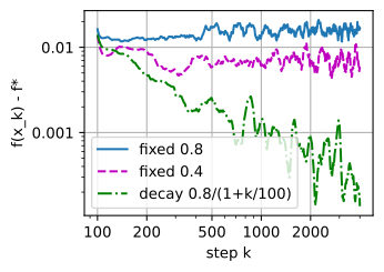
mean gap, last 1000 steps: 1.4e-02, 6.8e-03, 2.3e-04
floor(0.8) / floor(0.4) = 1.99, floor(0.8) / decay = 59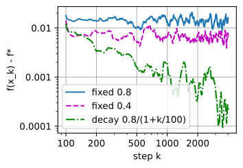
mean gap, last 1000 steps: 1.4e-02, 6.6e-03, 4.8e-04
floor(0.8) / floor(0.4) = 2.12, floor(0.8) / decay = 30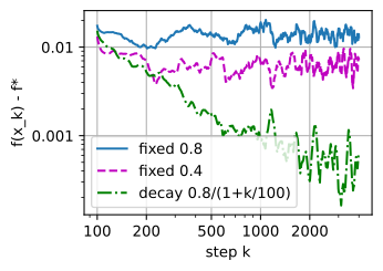
mean gap, last 1000 steps: 2.0e-02, 9.0e-03, 6.5e-04
floor(0.8) / floor(0.4) = 2.23, floor(0.8) / decay = 31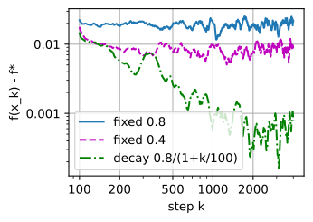
Both fixed steps stall. The mean gap over the last \(1{,}000\) steps is about \(1\) to \(2 \times 10^{-2}\) at \(\eta = 0.8\), and halving the step about halves it. The ratio scatters between about \(1.7\) and \(2.8\) across runs, around the factor \(2\) that the quadratic model predicts, although the loss is not quadratic. The decaying run ends roughly \(20\) to \(90\) times below the \(\eta = 0.8\) floor, and on the log–log plot its curve still trends down, jagged with minibatch noise. Its early large steps cover the distance to the minimizer, and its late small steps shrink the noise ball.
26.3.2.2 The Constant in a \(1/k\) Schedule
The schedule \(\eta_k = c/(k + k_0)\) satisfies both Robbins–Monro conditions for every \(c > 0\), and the shift \(k_0\) keeps the first steps below the stability ceiling. Does every \(c\) give the rate \(1/k\)? The scalar model with curvature \(\lambda = \mu\) answers exactly. Writing \(t = k + k_0\), its recursion becomes
\[ e_{k+1} = \Big(1 - \frac{c\mu}{t}\Big)^2 e_k + \frac{c^2 \sigma^2}{t^2}. \]
The contraction now weakens like \(1/t\), while the injected noise falls like \(1/t^2\). Which of the two wins depends on \(c\).
Proposition (the constant of a \(1/k\) schedule). On the scalar model with curvature \(\mu\) and steps \(\eta_k = c/(k + k_0)\), if \(2c\mu > 1\) then \(k\, e_k \to A\) with
\[ A = \frac{c^2 \sigma^2}{2c\mu - 1}. \tag{26.3.6}\]
If \(2c\mu < 1\), then \(e_k\) decays like \(k^{-2c\mu}\), more slowly than \(1/k\). For every \(c > 0\), \(e_k \to 0\).
Derivation of the constant. We find \(A\) to leading order; exercise 2 turns this into an induction. Substitute \(e_k \approx A/t\) into the recursion. The left side is \(A/(t+1) \approx A/t - A/t^2\). On the right, \((1 - c\mu/t)^2 \approx 1 - 2c\mu/t\), so the right side is \(A/t - 2c\mu A/t^2 + c^2\sigma^2/t^2\) up to terms of order \(t^{-3}\). The \(1/t\) terms agree, and matching the \(1/t^2\) terms gives \(-A = -2c\mu A + c^2\sigma^2\), that is, \(A(2c\mu - 1) = c^2\sigma^2\). The step that is not routine is the shift on the left: moving from \(t\) to \(t + 1\) contributes \(-A/t^2\), of the same order as the contraction, and it is the source of the threshold. Without it we would find \(A = c\sigma^2/(2\mu)\) for every \(c\).
Below the threshold, the contractions decide the rate, both for the initial error and for the noise injected early: their product is \(\prod_{j}(1 - c\mu/(j + k_0))^2 \approx (k_0/t)^{2c\mu}\), because \(\log(1 - u) \approx -u\) and \(\sum_{j \le t} 1/j \approx \log t\), and for \(2c\mu < 1\) this decays more slowly than \(1/t\). \(\blacksquare\)
Take \(\mu = \sigma = 1\). The constant \(c = 1\) gives \(A = 1\); iterating the recursion from \(e_0 = 1\) with \(k_0 = 10\) gives \(k\, e_k = 1.0001\) at \(k = 10^6\). The constant \(c = 2\) gives \(A = 4/3\) and \(c = 0.75\) gives \(A = 1.125\). Below the threshold, \(c = 0.25\) gives a log–log slope of \(-0.50\) between \(k = 10^5\) and \(10^6\), and \(c = 0.1\) a slope of \(-0.20\). The constant \(A\) is smallest at \(c = 1/\mu\), where \(A = \sigma^2/\mu^2\): the best \(1/k\) schedule reaches \(e_k \approx \sigma^2/(\mu^2 k)\). Averaging the iterates of a run with a small constant step reaches the same constant, with no decay at all (exercise 6).
Intuitively, with \(c < 1/(2\mu)\) the steps shrink faster than the iterate can use them, so the schedule limits the progress before the noise does. This is one reason practical schedules decay more slowly than \(1/k\).
On the running example the shift \(k_0\) cannot be small either. The first step must respect the stiff coordinate’s ceiling, \(c/k_0 < 2/L\), so \(k_0 > cL/2\), and the best constant for the slow coordinate, \(c = 1/\mu = 1\), forces \(k_0 > 500\). With \(k_0 = 1000\) and \(\mathbf{x}_0 = (1, 1)\), the slow coordinate’s transient still holds a fraction \((k_0/(k + k_0))^2 \approx 0.008\) of its initial value at \(k = 10^4\), and the expected loss ends at \(4.2 \times 10^{-3}\), more than five times the constant step’s floor of \(7.5 \times 10^{-4}\). The small early steps that the stiff coordinate demands leave the slow coordinate far from its minimizer, and the condition number reappears in \(k_0\).
26.3.2.3 Schedule Shapes under the Exact Recursion
Practice uses other shapes than \(1/k\), above all cosine decay and warmup–stable–decay. No theorem ranks them on a deep network. On the quadratic model, however, the expected loss of any schedule can be computed exactly, with no runs and no random numbers. The derivation of the floor holds step by step when the step size changes, so
\[ e_{k+1} = (1 - \eta_k \lambda)^2 e_k + \eta_k^2 \sigma^2, \qquad \mathbb{E} f(x_k) = \tfrac12 \lambda e_k. \]
Iterating this recursion computes the expected loss of a whole run in \(K\) multiplications. We compare four shapes over a budget of \(K\) steps, which Figure 26.3.2 draws. They are a constant step \(\eta_0\); the decay \(\eta_0/(1 + k/k_0)\); cosine decay (Loshchilov and Hutter 2016); and warmup–stable–decay (WSD) (Hu et al. 2024), which holds \(\eta_0\) for the first \(80\%\) of the budget and then decays linearly to zero:
\[ \eta_k^{\textrm{cos}} = \tfrac12 \eta_0 \Big(1 + \cos\frac{\pi k}{K}\Big), \qquad \eta_k^{\textrm{WSD}} = \begin{cases} \eta_0, & k < 0.8K, \\ \eta_0\, \dfrac{K - k}{0.2K}, & k \ge 0.8K. \end{cases} \]
Both start at \(\eta_0\) and end at zero; cosine decays throughout the run, WSD only at its end. WSD is popular for an operational reason: any checkpoint of its constant phase can be decayed to any budget, so the budget need not be fixed at launch. The quadratic model ranks the final losses of the shapes, not such operational merits.

Which shape ends lowest? The cell iterates the exact recursion with \(\lambda = \sigma = 1\), \(K = 2000\), \(\eta_0 = 0.3\) and \(x_0 = 3\) (without the warmup), prints the expected loss at \(80\%\) of the budget and at the end, and plots \(\mathbb{E} f(x_k)\).
lam, sigma, K, eta0, x0 = 1.0, 1.0, 2000, 0.3, 3.0

def expected_loss(schedule, lam, sigma, K, x0):
    """E f(x_k) = lam e_k / 2 for k = 1..K from the exact second-moment recursion."""
    e, Ef = x0**2, np.empty(K)
    for k in range(K):
        eta = schedule(k)
        e = (1 - eta * lam)**2 * e + eta**2 * sigma**2
        Ef[k] = 0.5 * lam * e
    return Ef

schedules = {
    'constant': lambda k: eta0,
    'c/k': lambda k: eta0 / (1 + k / 50),
    'cosine': lambda k: 0.5 * eta0 * (1 + np.cos(np.pi * k / K)),
    'WSD': lambda k: eta0 if k < 0.8 * K else eta0 * (K - k) / (0.2 * K)}
traces = {name: expected_loss(s, lam, sigma, K, x0) for name, s in schedules.items()}
print(f'floor {eta0 * sigma**2 / (2 * (2 - eta0 * lam)):.4f}   '
      + ''.join(f'{name:>10s}' for name in traces))
for label, k in [('E f at 80%', int(0.8 * K) - 1), ('E f at end', K - 1)]:
    print(f'{label:15s}' + ''.join(f'{Ef[k]:10.2e}' for Ef in traces.values()))
d2l.plot(np.arange(1, K + 1), list(traces.values()), 'step k', 'E f(x_k)',
yscale='log', legend=list(traces))floor 0.0882 constant c/k cosine WSD
E f at 80% 8.82e-02 2.36e-03 7.87e-03 8.82e-02
E f at end 8.82e-02 1.90e-03 1.68e-03 6.13e-03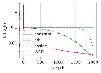
floor 0.0882     constant       c/k    cosine       WSD
E f at 80%       8.82e-02  2.36e-03  7.87e-03  8.82e-02
E f at end       8.82e-02  1.90e-03  1.68e-03  6.13e-03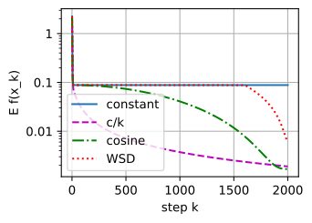
floor 0.0882     constant       c/k    cosine       WSD
E f at 80%       8.82e-02  2.36e-03  7.87e-03  8.82e-02
E f at end       8.82e-02  1.90e-03  1.68e-03  6.13e-03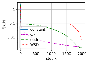
floor 0.0882     constant       c/k    cosine       WSD
E f at 80%       8.82e-02  2.36e-03  7.87e-03  8.82e-02
E f at end       8.82e-02  1.90e-03  1.68e-03  6.13e-03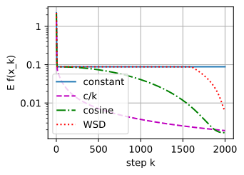
The output is the same on every run. The constant step comes within a tenth of its loss floor \(0.0882\) by step \(9\) and stays there. WSD is the constant run until its decay begins, so at \(80\%\) of the budget it sits on the same floor. Its last \(400\) steps lower the loss \(14.4\) times, to \(6.1 \times 10^{-3}\), so all of its improvement comes from the decay. Cosine and \(c/k\) end close together, at \(1.7 \times 10^{-3}\) and \(1.9 \times 10^{-3}\), and WSD ends three to four times higher.
The \(c/k\) value checks the proposition: the schedule \(0.3/(1 + k/50)\) is \(c/(k + k_0)\) with \(c = 15\) and \(k_0 = 50\), so \(A = 225/29 = 7.8\) and \(\mathbb{E} f(x_K) \approx \tfrac12 A/(K + k_0) = 1.9 \times 10^{-3}\). The ordering is exact for these parameters but does not carry over to a network, where WSD’s plateau is valued for the operational reason above. On the model itself, the plateau does not help the final loss: lengthening WSD’s decay phase lowers the final loss steadily, down to \(2.7 \times 10^{-3}\) for a linear decay over the whole run (exercise 8).
26.3.3 Rates for a Fixed Budget
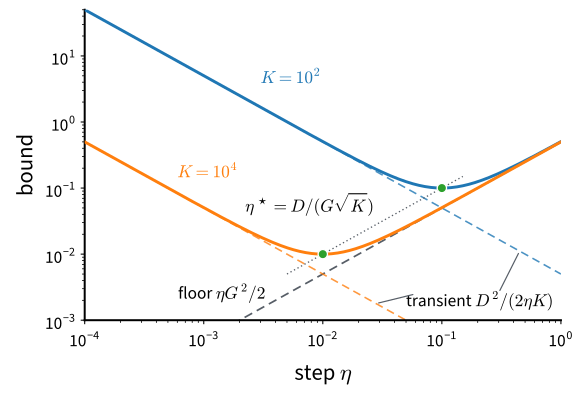
A decaying schedule is designed for a run of unlimited length. In practice the budget \(K\) is fixed in advance, and the question becomes which constant step to use and what loss it guarantees. Without strong convexity there is no contraction factor and no exact floor, so we bound instead of compute. Both results of this part have the same two-term shape: a transient that falls like \(1/(\eta K)\) plus a floor that grows like \(\eta\). The two terms balance at \(\eta \propto 1/\sqrt{K}\), as Figure 26.3.3 shows.
26.3.3.1 Averaged Iterates on Convex Losses
What can a constant step guarantee in \(K\) steps on a convex loss? The result needs only convexity, through the subgradient inequality: a vector \(\mathbf{s}\) is a subgradient of \(f\) at \(\mathbf{x}\) if \(f(\mathbf{y}) \ge f(\mathbf{x}) + \mathbf{s}^\top(\mathbf{y} - \mathbf{x})\) for all \(\mathbf{y}\), and the set \(\partial f(\mathbf{x})\) of subgradients is \(\{\nabla f(\mathbf{x})\}\) wherever \(f\) is differentiable (Section 26.2).
Proposition (SGD on a convex loss, averaged iterate). Let \(f\) be convex with a minimizer \(\mathbf{x}^\star\) and \(f^\star = f(\mathbf{x}^\star)\). Run \(\mathbf{x}_{k+1} = \mathbf{x}_k - \eta\, \mathbf{g}_k\) from a point with \(\|\mathbf{x}_0 - \mathbf{x}^\star\| \le D\), where the stochastic gradient satisfies \(\mathbb{E}[\mathbf{g}_k \mid \mathbf{x}_k] \in \partial f(\mathbf{x}_k)\) and \(\mathbb{E}[\|\mathbf{g}_k\|^2 \mid \mathbf{x}_k] \le G^2\). Then the average \(\bar{\mathbf{x}}_K = \frac1K \sum_{k=0}^{K-1} \mathbf{x}_k\) satisfies
\[ \mathbb{E}\big[f(\bar{\mathbf{x}}_K)\big] - f^\star \;\le\; \frac{D^2}{2\eta K} + \frac{\eta\, G^2}{2}, \tag{26.3.7}\]
and the step \(\eta = D/(G\sqrt{K})\) gives \(\mathbb{E}[f(\bar{\mathbf{x}}_K)] - f^\star \le DG/\sqrt{K}\).
Proof. We follow the squared distance to the minimizer. Expanding the step,
\[ \|\mathbf{x}_{k+1} - \mathbf{x}^\star\|^2 = \|\mathbf{x}_k - \mathbf{x}^\star\|^2 - 2\eta\, \mathbf{g}_k^\top(\mathbf{x}_k - \mathbf{x}^\star) + \eta^2 \|\mathbf{g}_k\|^2. \]
Take the expectation given \(\mathbf{x}_k\). The middle term becomes \(-2\eta\, \mathbf{s}_k^\top(\mathbf{x}_k - \mathbf{x}^\star)\) with the subgradient \(\mathbf{s}_k = \mathbb{E}[\mathbf{g}_k \mid \mathbf{x}_k]\), and the subgradient inequality at \(\mathbf{y} = \mathbf{x}^\star\) gives \(\mathbf{s}_k^\top(\mathbf{x}_k - \mathbf{x}^\star) \ge f(\mathbf{x}_k) - f^\star\). This is the step that is not routine: the inner product of the gradient with the displacement from the minimizer is at least the loss gap, so a large gap forces the distance down. The last term is at most \(\eta^2 G^2\). Taking total expectations and writing \(r_k = \mathbb{E}\|\mathbf{x}_k - \mathbf{x}^\star\|^2\),
\[ 2\eta\, \mathbb{E}\big[f(\mathbf{x}_k) - f^\star\big] \;\le\; r_k - r_{k+1} + \eta^2 G^2 . \]
Summing over \(k < K\) telescopes the distances, and \(r_0 - r_K \le D^2\), so \(2\eta \sum_{k<K} \mathbb{E}[f(\mathbf{x}_k) - f^\star] \le D^2 + K\eta^2 G^2\). Divide by \(2\eta K\) and apply Jensen’s inequality to the convex \(f\), \(f(\bar{\mathbf{x}}_K) \le \frac1K \sum_k f(\mathbf{x}_k)\). The two terms of the bound are equal at \(\eta = D/(G\sqrt{K})\), where each is \(DG/(2\sqrt{K})\). \(\blacksquare\)
The transient \(D^2/(2\eta K)\) is the distance that \(K\) steps of size \(\eta\) must cover, and the floor \(\eta G^2/2\) is the noise that each step injects. The proof needs no smoothness, so the loss may have corners, as the hinge loss does. With \(D = G = 1\) and \(K = 10^4\), the best step is \(\eta = 0.01\) and the bound is \(0.01\); with \(K = 10^2\), the step is \(0.1\) and the bound \(0.1\). A hundred times the budget lowers both the best step and the bound tenfold. This is also the best possible order: over the class of the proposition, no method that sees only unbiased stochastic gradients with \(\mathbb{E}\|\mathbf{g}\|^2 \le G^2\) can guarantee less than a fixed positive multiple of \(DG/\sqrt{K}\) in the worst case (Nemirovski and Yudin 1983).
Strong convexity changes the order. On the scalar quadratic, the best constant step for a budget \(K\) reaches \(e_K = \Theta(\log K/K)\) (exercise 5), because the transient there decays geometrically, like \(\rho^{2K}\), rather than like \(1/(\eta K)\).
The proposition bounds the average of the iterates. The last iterate obeys a weaker bound, and for the last iterate the worst-case optimal schedule over a known budget decays linearly to zero (Defazio et al. 2023). The hypothesis \(\mathbb{E}\|\mathbf{g}_k\|^2 \le G^2\) also limits the result: it fails for a quadratic on all of \(\mathbb{R}^d\), whose gradient is unbounded. It holds for Lipschitz losses with bounded features, such as the logistic loss, or for iterates that stay in a bounded set. As a worst-case bound it can be loose on a particular problem: on the logistic problem of this section it overestimates the gap by more than an order of magnitude (exercise 10).
26.3.3.2 Random Iterates on Nonconvex Losses
Networks have nonconvex losses and noisy gradients, and the results so far handle one of these at a time. For a function \(f\) whose gradient is \(L\)-Lipschitz (an \(L\)-smooth function), the graph lies below a parabola of curvature \(L\) tangent at any point,
\[ f(\mathbf{y}) \;\le\; f(\mathbf{x}) + \nabla f(\mathbf{x})^\top(\mathbf{y} - \mathbf{x}) + \frac{L}{2}\|\mathbf{y} - \mathbf{x}\|^2 \quad \textrm{for all } \mathbf{x}, \mathbf{y}. \]
This quadratic ceiling bounds the loss after any step by the loss before it, a linear decrease, and a penalty for the length of the step. With exact gradients and \(\eta = 1/L\), the ceiling gives \(\min_{k<K}\|\nabla f(\mathbf{x}_k)\|^2 \le 2L\Delta/K\) without any convexity, where \(f^\star\) is a lower bound of \(f\) and \(\Delta = f(\mathbf{x}_0) - f^\star\) (Section 26.1). With noisy gradients on a quadratic, a fixed step parks on a floor. The theorem of Ghadimi and Lan (2013) combines the two. Model one SGD step as \(\mathbf{x}_{k+1} = \mathbf{x}_k - \eta\, \mathbf{g}_k\), where the stochastic gradient satisfies
\[ \mathbb{E}\left[\mathbf{g}_k \mid \mathbf{x}_k\right] = \nabla f(\mathbf{x}_k), \qquad \mathbb{E}\left[\|\mathbf{g}_k - \nabla f(\mathbf{x}_k)\|^2 \mid \mathbf{x}_k\right] \;\le\; \sigma^2. \tag{26.3.8}\]
On average the stochastic gradient points the right way, and its error has mean square at most \(\sigma^2\) wherever the iterate is. A minibatch gradient meets both conditions with \(\sigma^2 = \sup_{\mathbf{x}} \operatorname{tr}\boldsymbol{\Sigma}(\mathbf{x})/b\) by Equation 26.3.2, provided this supremum is finite. It is finite for the bounded \(\tanh\) model below; it is infinite for least squares on all of \(\mathbb{R}^d\), whose gradient noise grows with the distance from the minimizer.
Proposition (SGD finds approximate stationary points). Let \(f\) be \(L\)-smooth and bounded below by \(f^\star\), write \(\Delta = f(\mathbf{x}_0) - f^\star\), and run SGD with stochastic gradients satisfying Equation 26.3.8 and a constant step \(\eta \le 1/L\). Then
\[ \frac{1}{K} \sum_{k=0}^{K-1} \mathbb{E}\left[\|\nabla f(\mathbf{x}_k)\|^2\right] \;\le\; \frac{2\Delta}{\eta K} + L\eta\sigma^2, \tag{26.3.9}\]
and the step \(\eta = \min\bigl(1/L,\ \sqrt{2\Delta/(L\sigma^2 K)}\bigr)\) gives, for an index \(R\) drawn uniformly from \(\{0, \ldots, K-1\}\) independently of the run,
\[ \mathbb{E}\left[\|\nabla f(\mathbf{x}_R)\|^2\right] \;\le\; \frac{2L\Delta}{K} + 2\sigma\,\sqrt{\frac{2L\Delta}{K}}. \tag{26.3.10}\]
Proof. Apply the quadratic ceiling to the step actually taken, \(\mathbf{y} - \mathbf{x} = -\eta\, \mathbf{g}_k\):
\[ f(\mathbf{x}_{k+1}) \;\le\; f(\mathbf{x}_k) - \eta\, \nabla f(\mathbf{x}_k)^\top \mathbf{g}_k + \tfrac{L\eta^2}{2}\, \|\mathbf{g}_k\|^2. \]
Take the expectation given \(\mathbf{x}_k\). This is the step that is not routine: conditioning on the iterate turns the middle term into \(-\eta\,\|\nabla f(\mathbf{x}_k)\|^2\) by unbiasedness, and splits the last term into signal plus noise, \(\mathbb{E}[\|\mathbf{g}_k\|^2 \mid \mathbf{x}_k] = \|\nabla f(\mathbf{x}_k)\|^2 + \mathbb{E}[\|\mathbf{g}_k - \nabla f(\mathbf{x}_k)\|^2 \mid \mathbf{x}_k] \le \|\nabla f(\mathbf{x}_k)\|^2 + \sigma^2\). Collecting,
\[ \mathbb{E}\left[f(\mathbf{x}_{k+1}) \mid \mathbf{x}_k\right] \;\le\; f(\mathbf{x}_k) - \eta\left(1 - \tfrac{L\eta}{2}\right) \|\nabla f(\mathbf{x}_k)\|^2 + \tfrac{L\eta^2 \sigma^2}{2}. \]
This is the descent lemma of gradient descent with an extra variance term \(\tfrac12 L\eta^2\sigma^2\) per step. For \(\eta \le 1/L\) the bracket is at least \(\tfrac12\). Take total expectations and sum over \(k = 0, \ldots, K-1\): the losses telescope to \(\mathbb{E}[f(\mathbf{x}_K)] - f(\mathbf{x}_0) \ge -\Delta\), and dividing by \(\eta K/2\) gives Equation 26.3.9. The average over \(k\) is the expectation at the uniformly random index \(R\). For the balanced step there are two cases. If \(\sqrt{2\Delta/(L\sigma^2K)} \le 1/L\), the two terms of Equation 26.3.9 are equal, each \(\sigma\sqrt{2L\Delta/K}\). Otherwise \(\eta = 1/L\) and \(\sigma^2 < 2L\Delta/K\), so the bound is \(2L\Delta/K + \sigma^2 \le 2L\Delta/K + \sigma\sqrt{2L\Delta/K}\). Both are at most the stated bound. \(\blacksquare\)
With \(\sigma = 0\) the second term vanishes, and the deterministic rate \(2L\Delta/K\) returns. With noise and \(K > 2L\Delta/\sigma^2\), the case in which \(\eta < 1/L\), the second term is the larger one, and it decays like \(K^{-1/2}\). With \(L = \Delta = \sigma = 1\) and \(K = 10^4\), the step is \(\eta = 0.014\) and the bound is \(2 \times 10^{-4} + 0.028\): the noise term is \(140\) times the transient. At \(K = 10^6\) the step is \(0.0014\) and the bound \(0.0028\). The bound controls the squared gradient norm: a hundred times the budget gives ten times less \(\mathbb{E}\|\nabla f\|^2\), but a ten times smaller gradient norm needs \(10^4\) times the budget. With a biased estimator the proof leaves an extra inner product, and the bound acquires a term that does not shrink with \(K\) (exercise 4).
Why does the guarantee speak of a random iterate? With exact gradients the best iterate can be identified, since \(\|\nabla f(\mathbf{x}_k)\|\) is observed. With stochastic gradients it is not, so an algorithm cannot pick the iterate with the smallest gradient; drawing \(R\) at random is a choice it can make, and the average over the run is what that choice controls.
Compared with the convex case, the two terms and the step \(\eta \propto 1/\sqrt{K}\) are the same. The bound now controls a squared gradient at a random iterate instead of a function value at the average. Without convexity a small gradient is all that can be certified, and a stationary point need not be a minimizer. This rate is optimal as well: no method with access only to such stochastic gradients can guarantee a better order in the worst case over this class (Arjevani et al. 2023).
26.3.3.3 The Rate on a Single \(\tanh\) Neuron
Does \(\mathbb{E}\|\nabla f(\mathbf{x}_R)\|^2\) fall like \(K^{-1/2}\) when \(\eta \propto 1/\sqrt{K}\)? We measure it on a small nonconvex problem, a single \(\tanh\) neuron fit by least squares to noisy labels: \(n = 64\) examples in five dimensions and
\[ f(\mathbf{x}) = \frac1n \sum_{i=1}^n \big(\tanh(\mathbf{a}_i^\top \mathbf{x}) - y_i\big)^2 . \]
Each term is bounded and smooth, but the sum is not convex: \(\tanh\) flattens for large arguments, so the loss has plateaus. The cell defines the data and the exact gradient for a batch of iterates, one per row of \(\mathbf{X}\).
n_nc, d_nc = 64, 5                                # a small nonconvex problem
A_nc = rng.normal(size=(n_nc, d_nc))
y_nc = np.tanh(A_nc @ rng.normal(size=d_nc)) + 0.5 * rng.normal(size=n_nc)

def full_grad(X, A, y):
    """Exact gradient of mean_i (tanh(a_i^T x) - y_i)^2 at each row x of X."""
    t = np.tanh(X @ A.T)                          # (runs, n)
    return 2 * ((t - y) * (1 - t**2)) @ A / len(y)
The next cell runs SGD with single-example gradients for the budgets \(K = 125, 500, 2000, 8000\) with \(\eta = 0.5/\sqrt{K}\), twenty runs at a time as the rows of X. Along each run it records the average of \(\|\nabla f(\mathbf{x}_k)\|^2\), which is the random-iterate quantity, and its minimum, the best iterate. It prints both against \(K\) with their log–log slopes and plots the first with a reference line of slope \(-1/2\).
runs, Ks, avg, best = 20, np.array([125, 500, 2000, 8000]), [], []
for K in Ks:
    eta = 0.5 / np.sqrt(K)                        # the theorem's eta ~ 1/sqrt(K)
    X = np.zeros((runs, d_nc))                    # one row per independent run
    total, low = np.zeros(runs), np.full(runs, np.inf)
    for k in range(K):
        g2 = (full_grad(X, A_nc, y_nc)**2).sum(axis=1)   # |grad f(x_k)|^2
        total, low = total + g2, np.minimum(low, g2)
        i = rng.integers(0, n_nc, size=runs)             # one example per run
        t = np.tanh((X * A_nc[i]).sum(axis=1))
        X -= eta * (2 * (t - y_nc[i]) * (1 - t**2))[:, None] * A_nc[i]
    avg.append(total.mean() / K), best.append(low.mean())

def slope(v):
    return np.polyfit(np.log(Ks), np.log(v), 1)[0]

for name, v in [('random iterate', avg), ('best iterate', best)]:
    print(f'{name:15s}' + ' '.join(f'{u:.1e}' for u in v) + f'   slope {slope(v):.2f}')
d2l.plot(Ks, [avg, avg[0] * (Ks / Ks[0])**-0.5], 'budget K', 'E |grad f(x_R)|^2',
xscale='log', yscale='log', legend=['random iterate', 'slope -1/2'])random iterate 2.7e-01 1.2e-01 4.7e-02 2.1e-02 slope -0.62
best iterate 2.2e-02 4.8e-03 1.3e-03 2.6e-04 slope -1.05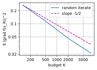
random iterate 2.1e-01 8.6e-02 3.7e-02 1.8e-02   slope -0.59
best iterate   1.5e-02 2.1e-03 2.9e-04 4.9e-05   slope -1.37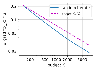
random iterate 1.8e-01 7.7e-02 3.1e-02 1.4e-02   slope -0.63
best iterate   1.1e-02 2.2e-03 3.6e-04 6.9e-05   slope -1.23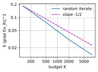
random iterate 2.1e-01 8.2e-02 3.7e-02 1.6e-02   slope -0.60
best iterate   1.8e-02 3.2e-03 6.8e-04 1.3e-04   slope -1.18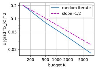
The random-iterate quantity falls by a factor of about \(12\) (between roughly \(9\) and \(16\) across runs) for a \(64\) times larger budget, a log–log slope of about \(-0.6\). The theorem gives an upper bound of slope \(-1/2\), so a slightly steeper measured slope is consistent with it. The best iterate falls faster, with a slope near \(-1\) or steeper, but noisy gradients do not tell us which iterate it is, so no guarantee can use it.
26.3.4 Variance Reduction
26.3.4.1 Control Variates
A decaying step removes the floor by shrinking \(\eta\), at the cost of slower progress. On a finite sum there is another way: remove the noise itself. At the minimizer the full gradient is zero, but each \(\nabla f_i(\mathbf{x}^\star)\) is not, and these nonzero example gradients are the noise that a fixed step keeps injecting. When a model fits every example exactly, they vanish, and on a strongly convex loss a fixed step then converges linearly with no correction (exercise 9).
The idea is to subtract from the noisy \(\nabla f_i(\mathbf{x})\) a quantity that moves with it and whose mean we know, and then add the mean back. A quantity of this kind is called a control variate. On a finite sum one is available: the gradient \(\nabla f_i(\tilde{\mathbf{x}})\) of the same example at a stored snapshot \(\tilde{\mathbf{x}}\), whose mean over \(i\) is the full gradient \(\nabla f(\tilde{\mathbf{x}})\), computed once per pass over the data. The SVRG estimator (stochastic variance-reduced gradient) (Johnson and Zhang 2013) is
\[ \tilde{\mathbf{g}}_i(\mathbf{x}) = \nabla f_i(\mathbf{x}) - \nabla f_i(\tilde{\mathbf{x}}) + \nabla f(\tilde{\mathbf{x}}). \tag{26.3.11}\]
It corrects the full gradient at the snapshot by the change of one example’s gradient between the snapshot and the current point. For a uniformly drawn index it is unbiased,
\[ \mathbb{E}_i\big[\tilde{\mathbf{g}}_i(\mathbf{x})\big] = \nabla f(\mathbf{x}) - \nabla f(\tilde{\mathbf{x}}) + \nabla f(\tilde{\mathbf{x}}) = \nabla f(\mathbf{x}), \]
and its advantage is its variance.
Proposition (the variance of the control variate vanishes at the optimum). If each \(f_i\) has an \(L_i\)-Lipschitz gradient and \(L_{\max} = \max_i L_i\), then for a uniformly drawn index \(i\)
\[ \mathbb{E}_i\big\|\tilde{\mathbf{g}}_i(\mathbf{x}) - \nabla f(\mathbf{x})\big\|^2 \;\le\; \mathbb{E}_i\big\|\nabla f_i(\mathbf{x}) - \nabla f_i(\tilde{\mathbf{x}})\big\|^2 \;\le\; L_{\max}^2\, \|\mathbf{x} - \tilde{\mathbf{x}}\|^2 . \tag{26.3.12}\]
Proof. The left side is the variance of the random vector \(\nabla f_i(\mathbf{x}) - \nabla f_i(\tilde{\mathbf{x}})\), whose mean is \(\nabla f(\mathbf{x}) - \nabla f(\tilde{\mathbf{x}})\); a variance is at most the second moment. Each term of the second moment is at most \(L_i^2\|\mathbf{x} - \tilde{\mathbf{x}}\|^2\) by the Lipschitz gradient. \(\blacksquare\)
The noise of the estimator is thus proportional to the distance between the iterate and the snapshot, so it vanishes as both approach \(\mathbf{x}^\star\), and a fixed step no longer has a floor. Intuitively, two gradients of the same example at nearby points share most of their noise. Their difference keeps the change, which is small, and discards the shared part, which is large.
26.3.4.2 SVRG and SAGA
The control variate needs a snapshot and its full gradient, and the snapshot must follow the iterate, or the distance in Equation 26.3.12 stops shrinking. A full gradient at every step would defeat the purpose. SVRG refreshes the snapshot once per epoch; SAGA replaces it by a table of stored gradients, refreshed one example at a time.
SVRG works in epochs. At the start of each epoch it stores a snapshot \(\tilde{\mathbf{x}}\) and computes the full gradient \(\nabla f(\tilde{\mathbf{x}})\); it then takes \(m\) inner steps \(\mathbf{x} \leftarrow \mathbf{x} - \eta\, \tilde{\mathbf{g}}_i(\mathbf{x})\) with fresh random indices, and the last inner iterate becomes the next snapshot. An epoch costs \(n + 2m\) example gradients. The guarantee of Johnson and Zhang (2013) (Theorem 1) needs three hypotheses: every \(f_i\) is convex with an \(L_{\max}\)-Lipschitz gradient, \(f\) is \(\mu\)-strongly convex, and the step satisfies \(\eta < 1/(4L_{\max})\) with an inner loop long enough for the theorem’s contraction factor to be below one. Under them, the expected gap \(\mathbb{E}[f(\tilde{\mathbf{x}})] - f^\star\) at the snapshot falls geometrically with the number of epochs. (The theorem takes a random inner iterate as the next snapshot; the last one behaves the same in practice.)
We test SVRG on ridge regression, a finite sum with \(f_i(\mathbf{x}) = \tfrac12(\mathbf{a}_i^\top\mathbf{x} - y_i)^2 + \tfrac{0.1}{2}\|\mathbf{x}\|^2\), \(n = 300\) examples and \(d = 12\) parameters. Its minimizer solves the normal equations, and each \(f_i\) has an \(L_i\)-Lipschitz gradient with \(L_i = \|\mathbf{a}_i\|^2 + 0.1\). The cell defines the data and the component and full gradients, and prints \(L_{\max}\).
n_r, d_r, reg_r = 300, 12, 0.1                    # ridge regression, a finite sum
A_r = rng.standard_normal((n_r, d_r))
y_r = A_r @ rng.standard_normal(d_r) + 0.5 * rng.standard_normal(n_r)
H_r = A_r.T @ A_r / n_r + reg_r * np.eye(d_r)     # Hessian of f
x_star_r = np.linalg.solve(H_r, A_r.T @ y_r / n_r)

def component_grad(x, i, A, y, reg):
    """Gradient of f_i(x) = (a_i^T x - y_i)^2 / 2 + reg |x|^2 / 2 (i: index or array)."""
    return A[i] * (A[i] @ x - y[i])[..., None] + reg * x

def full_grad_sum(x, A, y, reg):
    """Gradient of the finite sum f = mean_i f_i."""
    return A.T @ (A @ x - y) / len(y) + reg * x

def objective(x, A, y, reg):
    """The ridge objective f(x)."""
    return 0.5 * np.mean((A @ x - y)**2) + 0.5 * reg * x @ x

L_max = (A_r**2).sum(axis=1).max() + reg_r       # largest per-example smoothness
print(f'L_max = {L_max:.0f}, 1 / (4 L_max) = {1 / (4 * L_max):.4f}')L_max = 26, 1 / (4 L_max) = 0.0095L_max = 27, 1 / (4 L_max) = 0.0091L_max = 33, 1 / (4 L_max) = 0.0075L_max = 28, 1 / (4 L_max) = 0.0088\(L_{\max}\) is about \(30\) (typically between \(25\) and \(40\) across draws of the data), so the theorem asks for \(\eta\) below about \(0.008\).
Does a fixed step converge without a floor once the noise is cancelled? The cell runs SVRG with \(m = n\) and SGD with single-example gradients at the same fixed \(\eta = 0.02\), more than twice the theorem’s limit, for \(12\) epochs of \(3n\) example gradients each. It also predicts SGD’s floor from the first part of this section, as the sum of the loss floors \(\eta\sigma_i^2/(2(2 - \eta\lambda_i))\) over the eigenvectors of the Hessian, with \(\sigma_i^2\) the variance of the example gradients at \(\mathbf{x}^\star\) along eigenvector \(i\).
eta, epochs = 0.02, 12
f_star_r = objective(x_star_r, A_r, y_r, reg_r)
snap, gaps_svrg = np.zeros(d_r), []
for _ in range(epochs):                           # n + 2n example gradients per epoch
    g_snap = full_grad_sum(snap, A_r, y_r, reg_r)
    x = snap.copy()
    for i in rng.integers(0, n_r, size=n_r):
        x -= eta * (component_grad(x, i, A_r, y_r, reg_r)
                    - component_grad(snap, i, A_r, y_r, reg_r) + g_snap)
    snap = x
    gaps_svrg.append(objective(snap, A_r, y_r, reg_r) - f_star_r)
x, gaps_sgd = np.zeros(d_r), []
for _ in range(epochs):
    for i in rng.integers(0, n_r, size=3 * n_r):  # the same 3n budget per epoch
        x -= eta * component_grad(x, i, A_r, y_r, reg_r)
    gaps_sgd.append(objective(x, A_r, y_r, reg_r) - f_star_r)
G_r = component_grad(x_star_r, np.arange(n_r), A_r, y_r, reg_r)  # noise at x*
ev, Q = np.linalg.eigh(H_r)                       # Hessian eigenvalues, eigenvectors
s2 = ((G_r @ Q)**2).mean(axis=0)                  # noise variance per eigenvector
floor = (eta * s2 / (2 * (2 - eta * ev))).sum()   # the loss floors add
print(f'SGD: predicted floor {floor:.1e}, mean gap in epochs 4-12 '
      f'{np.mean(gaps_sgd[3:]):.1e}')
print('SVRG: gap after epochs 1, 4, 12: '
      + ', '.join(f'{gaps_svrg[e - 1]:.0e}' for e in (1, 4, 12)))
d2l.plot(np.arange(1, epochs + 1), [gaps_sgd, gaps_svrg], 'epoch (3n gradients)',
'f(x) - f*', yscale='log', legend=['SGD', 'SVRG'])SGD: predicted floor 2.2e-02, mean gap in epochs 4-12 3.1e-02
SVRG: gap after epochs 1, 4, 12: 8e-01, 2e-03, 1e-10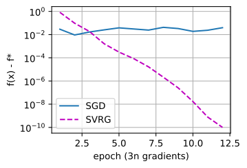
SGD: predicted floor 2.3e-02, mean gap in epochs 4-12 2.4e-02
SVRG: gap after epochs 1, 4, 12: 2e+00, 1e-03, 4e-11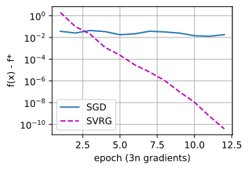
SGD: predicted floor 1.6e-02, mean gap in epochs 4-12 1.5e-02
SVRG: gap after epochs 1, 4, 12: 4e-01, 7e-04, 5e-11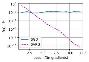
SGD: predicted floor 2.1e-02, mean gap in epochs 4-12 2.2e-02
SVRG: gap after epochs 1, 4, 12: 6e-01, 7e-04, 5e-11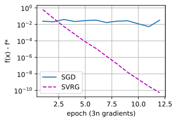
SGD drops quickly and then fluctuates at a few times \(10^{-2}\), where the floor formula of the first part puts it. The plateau usually lies between about \(10\%\) below and \(40\%\) above the prediction, always within a factor of two of it, and more often above. The formula counts only the noise at \(\mathbf{x}^\star\), and the example gradients spread more away from it. SVRG falls by a factor of about eight per epoch (between roughly five and thirteen across runs), to between about \(10^{-13}\) and \(10^{-8}\) by epoch \(12\). It does so at a step more than twice the theorem’s limit, so the theorem’s constants are loose. Three hypotheses carry this result: a finite sum, repeated passes over it, and strong convexity for the linear rate. On streaming data there is no sum to store.
SAGA (Defazio et al. 2014) replaces the snapshot by a table that holds the most recent gradient computed for each example, and uses the table’s average as the known mean. With \(\mathbf{t}_i\) the table entry of example \(i\), its estimator is \(\nabla f_i(\mathbf{x}) - \mathbf{t}_i + \tfrac1n\sum_j \mathbf{t}_j\), after which \(\mathbf{t}_i\) is overwritten by \(\nabla f_i(\mathbf{x})\). SAGA needs one new example gradient per step and no full passes, but stores \(n \times d\) numbers in this literal form. For a generalized linear model, where \(\nabla f_i\) is a scalar times \(\mathbf{a}_i\) plus a shared term, one scalar per example suffices (exercise 3).
Variance reduction differs from momentum. Momentum averages gradients across recent iterates and smooths high-frequency noise, but its average is biased for the gradient at the current point. SVRG and SAGA build an estimator that is unbiased at the current point and whose variance shrinks as the optimization converges. On deep networks these estimators have not given consistent gains: the control variate goes stale when the loss landscape changes under the iterate, for instance through data augmentation.
We can now measure the noise of a minibatch gradient, predict where a fixed step stalls and how soon, choose and compare decay schedules, tune a constant step to a budget, and cancel the noise of a finite sum. All of these methods share one step size across coordinates, so on the running example the stiff coordinate capped it at \(2/1000\) while the slow coordinate needed \(3{,}450\) steps to cut its transient a thousandfold. The next section lets each coordinate set its own step from the gradients it has seen.
26.3.5 Summary
A minibatch gradient is unbiased, and its error has power \(\operatorname{tr}\boldsymbol{\Sigma}/b\). On a quadratic, a fixed step \(\eta\) parks the second moment of each coordinate on the floor \(\eta\sigma^2/(\lambda(2 - \eta\lambda))\), reached geometrically at the rate \((1 - \eta\lambda)^2\), and the loss floors \(\eta\sigma^2/(2(2 - \eta\lambda))\) add over coordinates. The floor is linear in \(\eta\) while the transient decays faster for larger \(\eta\), so no fixed step reaches the minimizer, and every remedy trades the two. A Robbins–Monro schedule removes the floor, and \(\eta_k = c/k\) reaches \(O(1/k)\) only for \(c > 1/(2\mu)\). For a fixed budget \(K\), a constant step \(\eta \propto 1/\sqrt{K}\) gives \(DG/\sqrt{K}\) for the averaged iterate of a convex loss and, for large \(K\), \(O(\sigma\sqrt{L\Delta/K})\) for the squared gradient at a random iterate of a smooth nonconvex loss. On a finite sum, the SVRG estimator is unbiased with variance at most \(L_{\max}^2\|\mathbf{x} - \tilde{\mathbf{x}}\|^2\), so a fixed step converges linearly on a strongly convex loss; the next section replaces the single \(\eta\) by one step per coordinate.
26.3.6 Exercises
- [code] Noise scale and critical batch size. ● How much does one minibatch step lower the loss, and how does the gain depend on \(b\)? Write \(\mathbf{g} = \nabla f(\mathbf{x})\) and \(\mathbf{H} = \nabla^2 f(\mathbf{x})\), and approximate the loss after the step \(\mathbf{x} - \eta\,\hat{\mathbf{g}}_b\) of Equation 26.3.1 by its second-order Taylor expansion at \(\mathbf{x}\). The analysis follows McCandlish et al. (2018) .
Use the covariance \(\boldsymbol{\Sigma}/b\) of \(\hat{\mathbf{g}}_b\), established in the proof of Equation 26.3.2, to show that the expected loss after the step is minimized by \(\eta_{\textrm{opt}}(b) = \eta_{\max} / (1 + B_{\textrm{noise}}/b)\), with expected improvement \(\Delta_{\max} / (1 + B_{\textrm{noise}}/b)\), where
\[ \eta_{\max} = \frac{\|\mathbf{g}\|^2}{\mathbf{g}^\top \mathbf{H} \mathbf{g}}, \qquad \Delta_{\max} = \frac{\|\mathbf{g}\|^4}{2\,\mathbf{g}^\top \mathbf{H} \mathbf{g}}, \qquad B_{\textrm{noise}} = \frac{\operatorname{tr}(\mathbf{H} \boldsymbol{\Sigma})}{\mathbf{g}^\top \mathbf{H} \mathbf{g}}. \]
The linear scaling rule of Goyal et al. (2017) multiplies \(\eta\) by the same factor as \(b\). For which batch sizes does this rule follow from \(\eta_{\textrm{opt}}(b)\)? What does a larger batch gain per step once \(b \gg B_{\textrm{noise}}\)?
For \(\mathbf{H}\) proportional to the identity, \(B_{\textrm{noise}}\) reduces to \(B_{\textrm{simple}} = \operatorname{tr}\boldsymbol{\Sigma} / \|\mathbf{g}\|^2\), the gradient-noise scale \(b_{\textrm{noise}}\) of the text. Compute \(B_{\textrm{simple}}\) and \(B_{\textrm{noise}}\) for the logistic-regression problem of this section at \(\mathbf{x} = \mathbf{0}\) and after \(5\), \(10\), and \(20\) full-gradient steps with \(\eta = 0.5\), using
example_gradsand the Hessian \(\mathbf{H}(\mathbf{x}) = \frac1n \sum_i s_i(1 - s_i)\,\mathbf{a}_i \mathbf{a}_i^\top + 0.1\,\mathbf{I}\) with \(s_i = 1/(1 + e^{y_i \mathbf{a}_i^\top \mathbf{x}})\). How does the noise scale change as the iterates approach the optimum? Treat \(B_{\textrm{noise}}\) as the critical batch size that separates the two regimes of (b). How should the batch size change over a training run?
- [code] The constant in a \(1/k\) schedule. ●● The text found the constant \(A\) of Equation 26.3.6 to leading order. This exercise makes it rigorous and carries it to the running example.
- Let \(t = k + k_0\) and suppose \(u_{k+1} \le (1 - a/t)\, u_k + q/t^2\) for all \(k \ge 0\), with \(a > 1\), \(q > 0\), \(u_k \ge 0\) and \(k_0 \ge a\). Prove by induction that \(u_k \le \nu/(k + k_0)\) with \(\nu = \max\{q/(a - 1),\ k_0 u_0\}\). (Hint: \(1 - a/t \ge 0\), and \(1/t - 1/t^2 \le 1/(t + 1)\).)
- Apply the lemma to the recursion \(e_{k+1} = (1 - c\mu/t)^2 e_k + c^2\sigma^2/t^2\). Show that \((1 - c\mu/t)^2 \le 1 - (2c\mu - (c\mu)^2/k_0)/t\) for \(t \ge k_0\), so that any \(2c\mu > 1\) gives \(e_k = O(1/k)\) once \(k_0\) is large enough. Identify \(a\) and \(q\), and show that \(q/(a - 1) \to A\) as \(k_0 \to \infty\).
- For \(2c\mu < 1\), show \(e_k = \Theta(k^{-2c\mu})\) from the product \(\prod_{j<k}(1 - c\mu/(j + k_0))^2\) and the unrolled noise sum.
- Iterate the recursion with \(\mu = \sigma = 1\), \(k_0 = 10\) and \(e_0 = 1\) up to \(k = 10^6\) for \(c \in \{0.1, 0.25, 0.5, 1, 2\}\). Report the log–log slope between \(k = 10^5\) and \(10^6\) and the value of \(k\, e_k\) at \(10^6\). Which costs more, a constant twice the minimizer of \(A\) or half of it?
- On the running example \(\tfrac12(x_1^2 + 1000\,x_2^2)\) with unit noise per coordinate, stability at the first step forces \(c/k_0 < 2/1000\). Take \(c = 1/\mu = 1\), \(k_0 = 1000\), \(\mathbf{x}_0 = (1, 1)\) and \(K = 10^4\). Compute the expected loss by the two-coordinate recursion (it is about \(4.2 \times 10^{-3}\)) and compare it with the constant step \(\eta = 10^{-3}\) (\(7.5 \times 10^{-4}\)) and with cosine decay from the same \(\eta_0\) (\(1.0 \times 10^{-4}\)). Which coordinate does the \(1/k\) decay starve, and why does the condition number reappear in \(k_0\)?
- [code] SVRG inner loop and SAGA. Use the ridge data and the functions
component_grad,full_grad_sumandobjectiveof this section with a budget of \(36n = 10{,}800\) example-gradient evaluations, the budget behind the \(12\) reported epochs of the SVRG cell. Measure each run by the number of evaluations it needs to bring the gap below \(10^{-10}\), checking once per epoch.- Let the inner loop run \(m\) steps, so that one epoch costs \(n + 2m\) evaluations, and vary \(m \in \{10, 30, 75, 300, 1200\}\) at \(\eta \in \{0.01, 0.02\}\). Which \(m\) is best at each step size? Explain the trade-off between amortizing the snapshot gradient and letting the control variate go stale, and why the best \(m\) moves with \(\eta\).
- Implement SAGA: keep a table with the most recent gradient of every example, filled at \(\mathbf{x}_0\) for \(n\) evaluations, and use \(\nabla f_i(\mathbf{x}) - \mathbf{t}_i + \tfrac1n \sum_j \mathbf{t}_j\) as the estimator, where \(\mathbf{t}_i\) is the table entry of example \(i\). Compare SAGA with the best SVRG run at both step sizes. How many numbers does the table hold for this problem, and how many would suffice if you stored only the scalar \(\mathbf{a}_i^\top\mathbf{x} - y_i\) per example?
- Biased gradient estimators. ● Keep the variance bound of Equation 26.3.8, now measured around the conditional mean, but replace unbiasedness by \(\mathbb{E}[\mathbf{g}_k \mid \mathbf{x}_k] = \nabla f(\mathbf{x}_k) + \boldsymbol{\delta}_k\) with \(\|\boldsymbol{\delta}_k\| \le \delta\).
Redo the proof of Equation 26.3.9 for \(\eta \le 1/L\) and show
\[\frac{1}{K} \sum_{k=0}^{K-1} \mathbb{E}\left[\|\nabla f(\mathbf{x}_k)\|^2\right] \;\le\; \frac{2\Delta}{\eta K} + L\eta\sigma^2 + \delta^2. \tag{26.3.13}\]
Use \(L\eta \le 1\) on the term \(\tfrac{L\eta^2}{2}\|\nabla f(\mathbf{x}_k) + \boldsymbol{\delta}_k\|^2\) before expanding it.
Show that the term \(\delta^2\) cannot be removed: give a one-dimensional \(f\) and a constant bias for which SGD with \(\sigma = 0\) converges to a point where \(|f'|^2 = \delta^2\).
A single minibatch drawn uniformly without replacement is still an unbiased estimator of the full gradient. Which of the following estimators are biased in this sense: the example gradient at a step of random reshuffling (Section 9.3), which visits every example once per epoch in a fresh random order; a stochastic gradient clipped to a fixed maximum norm; the gradient evaluated at the iterate of \(\tau\) steps earlier, as in asynchronous training?
- [code] The best constant step for a budget. ● On the scalar model with \(\lambda = \sigma = 1\) and \(e_0 = 1\), Equation 26.3.3 gives \(e_K = (1 - \eta)^{2K}(1 - V) + V\) with \(V = \eta/(2 - \eta)\).
- Show that the minimizing step satisfies \(\eta^\star = \Theta(\log K/K)\) and that \(\min_\eta e_K = \Theta(\log K/K)\). (Hint: use \((1 - \eta)^{2K} \approx e^{-2\eta K}\) and \(V \approx \eta/2\), and set the derivative to zero.)
- Minimize numerically for \(K = 10^2, 10^3, 10^4\) (you should find \(\eta^\star \approx 0.030, 0.0041, 0.0005\) and \(e_K \approx 1.7 \times 10^{-2}, 2.3 \times 10^{-3}, 2.9 \times 10^{-4}\)), and check that \(\eta^\star K/\log K\) and \(e_K K/\log K\) stay of order one.
- Apply the budget rule \(\eta = 1/\sqrt{K}\) of the convex bound to this quadratic anyway. Show that \(e_K \approx 1/(2\sqrt{K})\), worse than (b) by a factor \(\Theta(\sqrt{K}/\log K)\).
- Which term of the bound Equation 26.3.7 does strong convexity improve, and why does that change the best step from \(\propto 1/\sqrt{K}\) to \(\propto \log K/K\)?
- [code] Iterate averaging. ● Polyak and Juditsky (1992) showed that averaging the iterates of a slowly decaying or constant-step run reaches the best possible constant. Consider the scalar model with a constant step \(\eta \in (0, 2/\lambda)\), started in its stationary distribution.
- Show that \(\textrm{Cov}(x_j, x_k) = V\rho^{|j - k|}\).
- Show that the average \(\bar{x}_K = \frac1K \sum_{k<K} x_k\) has \(\mathbb{E}[\bar{x}_K^2] = \frac{V}{K}\cdot\frac{1 + \rho}{1 - \rho} - O(K^{-2})\), and that \(V(1 + \rho)/(1 - \rho) = \sigma^2/\lambda^2\) for every such \(\eta\): to leading order the averaged iterate does not depend on the step.
- Check by simulation with \(K = 2000\) and \(4{,}000\) runs at \(\eta = 0.3\) and \(\eta = 0.1\), with \(\lambda = \sigma = 1\). You should find \(\mathbb{E}[\bar{x}_K^2] \approx 5 \times 10^{-4}\) in both cases, against last-iterate floors of \(0.18\) and \(0.053\).
- Started at \(x_0 = 3\) instead, the average remembers the transient. Show that its contribution to \(\mathbb{E}[\bar{x}_K^2]\) is about \((x_0/(\eta\lambda K))^2\), and decide when averaging only the second half of the run is better.
- Compare with the best \(1/k\) schedule, whose constant is \(A = \sigma^2/\mu^2\). What does each of the two routes to the rate \(\sigma^2/(\mu^2 K)\) require?
- Which Robbins–Monro condition does the quadratic need? ● On the scalar model with steps \(\eta_k\) and \(\rho_j = 1 - \eta_j\lambda\):
- Unroll the recursion to \(e_k = \prod_{j<k}\rho_j^2\, e_0 + \sigma^2 \sum_{j<k} \eta_j^2 \prod_{j<i<k} \rho_i^2\).
- Show that \(e_k \to 0\) whenever \(\eta_k \to 0\), \(\sum_k \eta_k = \infty\) and \(0 < \eta_k < 2/\lambda\): the square-summable condition is not needed for convergence in mean square on this model. (Hint: split the sum at an index \(m\) beyond which \(\eta_j \le \epsilon\), and compare the tail with the floor of the step \(\epsilon\).)
- For \(\eta_k = c/\sqrt{k}\), show that \(e_k \approx c\sigma^2/(2\lambda\sqrt{k})\), and check numerically with \(\lambda = \sigma = 1\) and \(c = 0.5\) (\(2.5 \times 10^{-3}\) at \(k = 10^4\), \(2.5 \times 10^{-4}\) at \(10^6\)).
- In words: what does \(\sum_k \eta_k^2 < \infty\) provide in the general theorem, which claims convergence for almost every run with noise that need not be additive? (Consider the accumulated noise \(\sum_k \eta_k \xi_k\).)
- [code] The decay fraction of WSD. Use the exact recursion of the schedule cell (\(\lambda = \sigma = 1\), \(K = 2000\), \(\eta_0 = 0.3\), \(x_0 = 3\)).
- Tabulate the final expected loss of WSD for the decay fractions \(0.05, 0.1, 0.2, 0.3, 0.5, 0.7, 0.9, 1\). (It falls steadily from \(1.24 \times 10^{-2}\) to \(2.73 \times 10^{-3}\).)
- A linear decay over the whole run ends at \(2.73 \times 10^{-3}\), cosine at \(1.68 \times 10^{-3}\). Explain the difference from the shapes of the two schedules near the end of the run.
- On this model the plateau gives no advantage in final loss. State what it gives in practice, and why a model with one fixed curvature and stationary noise cannot show it.
- [code] Interpolation and linear convergence. ●● Suppose each \(f_i\) is convex with an \(L_i\)-Lipschitz gradient, \(f\) is \(\mu\)-strongly convex, and every \(f_i\) is minimized at the same point \(\mathbf{x}^\star\), as when a model fits every training example exactly. The analysis follows Vaswani et al. (2019) .
- Show that \(\mathbb{E}_i\|\nabla f_i(\mathbf{x})\|^2 \le 2L_{\max}(f(\mathbf{x}) - f^\star)\). (Hint: a convex \(L\)-smooth \(h\) minimized at \(\mathbf{x}^\star\) satisfies \(\|\nabla h(\mathbf{x})\|^2 \le 2L(h(\mathbf{x}) - h(\mathbf{x}^\star))\).)
- Deduce that single-example SGD with a constant \(\eta \le 1/L_{\max}\) satisfies \(\mathbb{E}\|\mathbf{x}_{k+1} - \mathbf{x}^\star\|^2 \le (1 - \eta\mu)\,\mathbb{E}\|\mathbf{x}_k - \mathbf{x}^\star\|^2\): linear convergence with no floor. What is \(\operatorname{tr}\boldsymbol{\Sigma}(\mathbf{x}^\star)\) in this case?
- Check it on least squares with \(n = 50\) examples and \(d = 100\) parameters, \(\eta = 1/L_{\max}\) and \(\mathbf{x}_0 = \mathbf{0}\). The iterates stay in the row space of \(\mathbf{A}\), where \(f\) is strongly convex, so (b) applies there. Show that the gap falls linearly with consistent labels and also with labels corrupted by noise of standard deviation \(0.5\), and explain why the noise does not matter here.
- Repeat with \(n = 200\) and \(d = 100\). Now the noisy labels bring the floor back. Why?
- [code] The convex bound on the logistic problem. For the logistic-regression problem of this section:
- Set \(D = \|\mathbf{x}^\star\|\) for the reference optimum
x_star, and bound \(G^2\) on the ball of radius \(2D\) around the origin from \(\|\nabla f_i(\mathbf{x})\| \le \|\mathbf{a}_i\| + 0.1\,\|\mathbf{x}\|\). - Run SGD with \(b = 1\), \(\eta = D/(G\sqrt{K})\) and \(K = 4000\), check that the iterates stay in the ball, and compare the gap of the averaged iterate with the bound \(DG/\sqrt{K}\). By what factor is the bound loose?
- Which inequalities of the proof are loose here? The regularizer makes \(f\) strongly convex with \(\mu \ge 0.1\); what rate does that allow instead?
- Compare the last iterate with the average at the same \(\eta\).
- Set \(D = \|\mathbf{x}^\star\|\) for the reference optimum