rng = np.random.default_rng()36.2 Joint Distributions and Transformations
The dart of Section 36.1 was reduced to one number, its distance \(R\) from the center of a board of radius \(1\), with density \(2r\). But a dart lands at a point, and a point has two coordinates, a horizontal \(X\) and a vertical \(Y\). Most of what we model comes in such groups. An image is thousands of pixels whose values depend on each other, and every supervised problem is a pair, an input and a target. One density per variable cannot describe a group, because it is silent on how the variables move together.
Two questions occupy this section. The first is what one variable tells us about another. If the dart lands near the top of the board, at \(Y=0.9\), then \(X\) must lie within \(0.44\) of the center line, so \(Y\) certainly carries information about \(X\). Yet we will find that the best guess for \(X\) is \(0\) whatever \(Y\) is, and that the covariance of the two is zero. Dependence, predictability and correlation are three different things, and it takes the density of the pair to tell them apart. The second question is what a transformation does to a density, as when a layer acts on its input or a sampler on its noise. The dart’s distance can be drawn as \(R=\sqrt U\) from a uniform \(U\), and the square root has turned a flat density into \(2r\). Evidently a map does more to a density than relabel its axis.
Three results carry most of the weight later in the book: the law of total variance Equation 36.2.5, the conditional mean as the best squared-error predictor Equation 36.2.6, and the change of variables Equation 36.2.14. The covariance matrix and the remark that a correlation is a cosine can be skipped on a first reading.
36.2.1 Joint and Conditional Densities
Everything that can be asked about a pair is answered by one function of two arguments. We define it, and then extract three things from it: the distribution of one coordinate alone, the distribution of one coordinate once the other is known, and the average of one given the other, which is what a regression model estimates.
36.2.1.1 Joint and Marginal Densities
The density extends to two variables with small squares in place of short intervals. The joint density \(p_{X,Y}\) of a pair \((X,Y)\) is probability per unit area: a small square of side \(\epsilon\) at \((x,y)\) has probability about its area times the density,
\[ P\bigl(X\in[x,x+\epsilon],\ Y\in[y,y+\epsilon]\bigr)\approx\epsilon^2\,p_{X,Y}(x,y). \]
As for one variable, slicing a region into such squares leads to the property that we take as the definition: \(p_{X,Y}\ge0\), and \(P((X,Y)\in\mathcal{D})=\iint_{\mathcal{D}} p_{X,Y}(x,y)\,dx\,dy\) for a region \(\mathcal D\) of the plane, so that the total volume under the joint density is one. For \(n\) variables the same holds with \(n\)-dimensional boxes.
The dart’s position has the joint density \(p_{X,Y}(x,y)=1/\pi\) on the unit disk and \(0\) outside, since every part of the board is equally likely and the board has area \(\pi\). Although it is constant on the disk, it is not a function of \(x\) times a function of \(y\): the edge of the board ties the two coordinates together.
Often we hold a joint density but want the distribution of one coordinate alone, its marginal distribution. A thin vertical strip \(X\in[x,x+\epsilon]\) has probability about \(\epsilon\,p_X(x)\). Slicing the strip into squares in \(y\) and adding their probabilities,
\[ \epsilon\,p_X(x) \approx \sum_i P\bigl(X\in[x,x{+}\epsilon],\ Y\in[\epsilon i,\epsilon(i{+}1)]\bigr) \approx \sum_i \epsilon^{2}\,p_{X,Y}(x,\epsilon i). \]
Cancelling one \(\epsilon\) and recognizing the remaining sum as a Riemann sum in \(y\),
\[ p_X(x) = \int_{-\infty}^\infty p_{X, Y}(x, y)\,dy. \tag{36.2.1}\]
The marginal density at \(x\) is the joint density integrated up the vertical strip at \(x\), as in Figure 36.2.1. We integrate out the variable we do not care about. For the dart, the strip at \(x\) crosses the board from \(-\sqrt{1-x^2}\) to \(\sqrt{1-x^2}\), so
\[ p_X(x)=\int_{-\sqrt{1-x^2}}^{\sqrt{1-x^2}}\frac1\pi\,dy=\frac2\pi\sqrt{1-x^2}, \qquad -1\le x\le 1, \]
a semicircle. As a check, \(\int_{-1}^1\sqrt{1-x^2}\,dx\) is the area of half the unit disk, \(\pi/2\), so the marginal integrates to \(1\). The joint density is flat, but the marginal is not: a strip through the middle of the board is longer than one near the edge.

36.2.1.2 Conditional Densities and Independence
Once we learn that \(Y=y\), how should the density of \(X\) change? For discrete variables the answer is \(P(X=x\mid Y=y)=P(X=x,Y=y)/P(Y=y)\). With densities this formula divides zero by zero, because \(P(Y=y)=0\). The way out is the one that defined the density. We condition on a thin horizontal strip \(Y\in[y,y+\epsilon]\), which has positive probability, and let the strip shrink. By the square approximation and the one-variable rule,
\[ P\bigl(X\in[x,x+\epsilon]\bigm| Y\in[y,y+\epsilon]\bigr) \approx\frac{\epsilon^2\,p_{X,Y}(x,y)}{\epsilon\,p_Y(y)} =\epsilon\,\frac{p_{X,Y}(x,y)}{p_Y(y)}. \]
Inside the strip, the probability of a short \(x\)-interval is its length times \(p_{X,Y}(x,y)/p_Y(y)\). This ratio is the probability per unit length of \(X\) given \(Y=y\), and we define the conditional density
\[ p_{X\mid Y}(x\mid y) = \frac{p_{X,Y}(x,y)}{p_Y(y)}, \qquad p_Y(y) > 0. \tag{36.2.2}\]
For each \(y\) it is a density in \(x\): it is non-negative, and by the marginal rule Equation 36.2.1 it integrates to \(p_Y(y)/p_Y(y)=1\). Geometrically, we cut the joint density along the line \(Y=y\) and rescale the profile to unit area. For the dart, the line \(Y=y\) crosses the board on \([-\sqrt{1-y^2},\sqrt{1-y^2}]\), and
\[ p_{X\mid Y}(x\mid y)=\frac{1/\pi}{(2/\pi)\sqrt{1-y^2}}=\frac{1}{2\sqrt{1-y^2}} \qquad\textrm{for } |x|\le\sqrt{1-y^2}. \]
Given \(Y=y\), the horizontal position is uniform on the chord at height \(y\). The chord shrinks as \(|y|\) grows, so learning \(Y\) changes the distribution of \(X\).
Rearranging Equation 36.2.2 gives the chain rule \(p_{X,Y}(x,y)=p_{X\mid Y}(x\mid y)\,p_Y(y)\). Writing it both ways, \(p_{X\mid Y}\,p_Y=p_{Y\mid X}\,p_X\), and solving for \(p_{X\mid Y}\) gives Bayes’ rule for densities,
\[ p_{X\mid Y}(x\mid y) = \frac{p_{Y\mid X}(y\mid x)\,p_X(x)}{p_Y(y)}. \tag{36.2.3}\]
It turns a model of how \(Y\) arises from \(X\) into a statement about \(X\) after seeing \(Y\), as Bayes’ theorem did for discrete variables in Section 1.6.
In the special case where learning \(Y\) tells us nothing about \(X\), that is, \(p_{X\mid Y}(x\mid y)=p_X(x)\) whenever \(p_Y(y)>0\), the two variables are called independent, written \(X\perp Y\). By the chain rule this is the same as saying that the joint density factorizes, \(p_{X,Y}(x,y)=p_X(x)\,p_Y(y)\) (up to sets of probability zero): multiply by \(p_Y(y)\) to go one way and divide by it to go the other.
Independence means that the conditional density of \(X\) is the same function of \(x\), with the same location and the same shape, at every \(y\). Take the joint density \(p_{X,Y}(x,y)=4xy\) on the unit square \([0,1]^2\). Its marginal is \(p_Y(y)=\int_0^1 4xy\,dx=2y\), so \(p_{X\mid Y}(x\mid y)=4xy/(2y)=2x\), the same for every \(y\), and \(X\perp Y\). The dart is the opposite case: its conditional density is uniform at every \(y\), but on a chord whose length depends on \(y\).
Figure 36.2.2 shows that a common shape is not enough. For a correlated pair, the conditional densities at three heights have the same shape but different centers, so the pair is dependent; only when the joint factorizes do the three coincide.

Independence also gives the density of a sum. The pair \((X,X+Y)\) has the joint density \(p_X(x)\,p_Y(s-x)\) at \((x,s)\), and integrating out \(x\) as in Equation 36.2.1 leaves the convolution \(p_{X+Y}(s)=\int p_X(x)\,p_Y(s-x)\,dx\).
36.2.1.3 Conditional Expectation
A regression model predicts a target from an input. We keep the letters of the previous subsection, so here the target is \(X\) and the input, the variable we observe, is \(Y\); the main text writes the pair the other way round. Training with the squared loss looks for the function \(h\) that makes \(\mathbb{E}[(X-h(Y))^2]\) small. Which function is best? Within a thin strip \(Y\approx y\) the model must predict one number for a whole spread of targets. The number \(c\) closest on average, in squared distance, to a variable \(X\) is its mean, since expanding the square around \(\mu_X\) gives \(\mathbb{E}[(X-c)^2]=\textrm{Var}(X)+(\mu_X-c)^2\). This suggests predicting the average of \(X\) within the strip. The conditional expectation of \(X\) given \(Y=y\) is the mean of the conditional density,
\[ \mathbb{E}[X\mid Y{=}y] = \int x\,p_{X\mid Y}(x\mid y)\,dx. \tag{36.2.4}\]
It is the average of \(X\) among the outcomes with \(Y=y\). As \(y\) varies it traces a function of \(y\); evaluated at the random \(Y\), it becomes a random variable \(\mathbb{E}[X\mid Y]\) that depends on \(Y\) alone. The same strip average defines \(\mathbb{E}[g(X,Y)\mid Y{=}y]=\int g(x,y)\,p_{X\mid Y}(x\mid y)\,dx\) for any function \(g\). A factor \(h(Y)\) is constant within each strip, so it comes out of the average:
\[ \mathbb{E}[h(Y)\,g(X,Y)\mid Y]=h(Y)\,\mathbb{E}[g(X,Y)\mid Y]. \]
The spread within a strip is the conditional variance \(\textrm{Var}(X\mid Y)=\mathbb{E}[X^2\mid Y]-(\mathbb{E}[X\mid Y])^2\), the computational form Equation 36.1.9 applied within each strip.
Averaging the strip averages should give back the overall average, and the overall spread should split into a spread within strips and a spread between them. Both are true, and the second is the more useful.
Proposition (laws of total expectation and variance). Let \(X,Y\) have a joint density, and let \(X\) have finite variance (for discrete pairs, the same identities hold with integrals replaced by sums). Then
\[ \mathbb{E}[X] = \mathbb{E}\bigl[\mathbb{E}[X\mid Y]\bigr], \qquad \textrm{Var}(X) = \mathbb{E}\bigl[\textrm{Var}(X\mid Y)\bigr] + \textrm{Var}\bigl(\mathbb{E}[X\mid Y]\bigr). \tag{36.2.5}\]
Proof. For the first identity, the tower property, write out the inner mean and use the chain rule \(p_{X\mid Y}(x\mid y)\,p_Y(y)=p_{X,Y}(x,y)\) to put the strips back together into the joint density:
\[ \mathbb{E}\bigl[\mathbb{E}[X\mid Y]\bigr] = \int\!\Bigl(\int x\,p_{X\mid Y}(x\mid y)\,dx\Bigr)p_Y(y)\,dy = \iint x\,p_{X,Y}(x,y)\,dx\,dy = \mathbb{E}[X]. \]
The values of \(y\) with \(p_Y(y)=0\), where the conditional density is undefined, contribute to neither side: \(Y\) lands there with probability zero. The same computation with \(g(x,y)\) in place of \(x\) gives \(\mathbb{E}\bigl[\mathbb{E}[g(X,Y)\mid Y]\bigr]=\mathbb{E}[g(X,Y)]\). For the second identity, expand both terms on the right. By the tower property applied to \(X^2\),
\[ \mathbb{E}\bigl[\textrm{Var}(X\mid Y)\bigr] =\mathbb{E}\bigl[\mathbb{E}[X^2\mid Y]\bigr]-\mathbb{E}\bigl[(\mathbb{E}[X\mid Y])^2\bigr] =\mathbb{E}[X^2]-\mathbb{E}\bigl[(\mathbb{E}[X\mid Y])^2\bigr]. \]
By the computational form Equation 36.1.9 applied to the variable \(\mathbb{E}[X\mid Y]\), whose mean is \(\mathbb{E}[X]\) by the tower property,
\[ \textrm{Var}\bigl(\mathbb{E}[X\mid Y]\bigr) =\mathbb{E}\bigl[(\mathbb{E}[X\mid Y])^2\bigr]-\mathbb{E}[X]^2 . \]
Adding the two lines, the term \(\mathbb{E}[(\mathbb{E}[X\mid Y])^2]\) cancels and leaves \(\mathbb{E}[X^2]-\mathbb{E}[X]^2=\textrm{Var}(X)\). \(\blacksquare\)
The second identity is sometimes called Eve’s law, after the pattern E, V, V, E of its right side. It splits the spread of \(X\) into the average spread within each strip, the part that knowing \(Y\) cannot remove, and the spread of the strip averages, the part that \(Y\) explains. Statisticians use this split to attribute the variation in data to groups, under the name analysis of variance. The split also answers the regression question.
Proposition (the conditional mean is the best squared-error predictor). Let \(X\) have finite variance, and let \(h\) be any function with \(\mathbb{E}[h(Y)^2]<\infty\). Then
\[ \mathbb{E}\bigl[(X-h(Y))^2\bigr] =\mathbb{E}\bigl[\textrm{Var}(X\mid Y)\bigr] +\mathbb{E}\bigl[(\mathbb{E}[X\mid Y]-h(Y))^2\bigr]. \tag{36.2.6}\]
Proof. Write \(m(Y)=\mathbb{E}[X\mid Y]\) and split the error into two parts, \(X-h(Y)=(X-m(Y))+(m(Y)-h(Y))\). Squaring gives two squares and a cross term, and the cross term is the only step that needs thought. The mean of the first square is \(\mathbb{E}[\textrm{Var}(X\mid Y)]\) by the tower property. The cross term \(2(X-m(Y))(m(Y)-h(Y))\) has conditional mean zero, because the factor \(m(Y)-h(Y)\) depends on \(Y\) alone and comes out of the strip average, leaving \(\mathbb{E}[X-m(Y)\mid Y]=m(Y)-m(Y)=0\). By the tower property its mean is zero too. \(\blacksquare\)
The first term does not depend on \(h\), and the second is never negative and vanishes for \(h(Y)=\mathbb{E}[X\mid Y]\). So the conditional mean is the best predictor in squared error, and no predictor can do better than the average spread within the strips. A network trained with the squared loss is estimating \(\mathbb{E}[\textrm{target}\mid\textrm{input}]\), which is how Section 2.1 reads its model, there written \(\mathbb{E}[y\mid\mathbf x]\).
Two examples show the split with numbers. For the dart, predict \(X\) from \(Y\). Given \(Y=y\), \(X\) is uniform on a chord symmetric about \(0\), so \(\mathbb{E}[X\mid Y=y]=0\). A variable uniform on an interval of half-width \(w\) has variance \(w^2/3\), so \(\textrm{Var}(X\mid Y=y)=(1-y^2)/3\). By symmetry \(\mathbb{E}[X^2]=\mathbb{E}[Y^2]=\tfrac12\mathbb{E}[R^2]=\tfrac14\), and Eve’s law gives
\[ \textrm{Var}(X)=\mathbb{E}\Bigl[\frac{1-Y^2}{3}\Bigr]+\textrm{Var}(0) =\frac{1-1/4}{3}+0=\frac14 . \]
All of the variance is unexplained. Knowing \(Y\) narrows the range of \(X\) but never shifts its center, so the best predictor of \(X\) from \(Y\) is the constant \(0\), although \(X\) and \(Y\) are dependent.
For the second example, draw a label \(Z\) that is \(1\) with probability \(0.2\) and \(0\) with probability \(0.8\). Given \(Z=1\), draw \(X\) from the normal distribution \(\mathcal N(3,1)\) with mean \(3\) and variance \(1\), and given \(Z=0\) from \(\mathcal N(-1,1)\). This mixture has the two-bump density of Figure 36.1.1. Its mean is \(0.2\cdot3+0.8\cdot(-1)=-0.2\). Within each component the variance is \(1\), so \(\mathbb{E}[\textrm{Var}(X\mid Z)]=1\). Between the components, \(\mathbb{E}[X\mid Z]\) takes the values \(3\) and \(-1\), whose variance is \(0.2\cdot0.8\cdot(3-(-1))^2=2.56\). The total variance is \(3.56\), and the label explains \(2.56/3.56=72\%\) of it. In a sample of a million draws the two parts will come out near \(1\) and \(2.56\). Should their sum match the variance of the sample only as roughly as the parts match their targets, or exactly?
n = 10**6
z = rng.uniform(size=n) < 0.2                          # component label Z
x = np.where(z, rng.normal(3, 1, n), rng.normal(-1, 1, n))
w = np.array([np.mean(~z), np.mean(z)])                # P(Z=0), P(Z=1)
cond_mean = np.array([x[~z].mean(), x[z].mean()])      # E[X | Z]
within = w @ np.array([x[~z].var(), x[z].var()])       # E[Var(X | Z)]
between = w @ (cond_mean - x.mean())**2                # Var(E[X | Z])
print(f'Var(X) {x.var():.3f} = within {within:.3f} + between {between:.3f}')Var(X) 3.562 = within 1.000 + between 2.562Var(X) 3.560 = within 0.996 + between 2.563Var(X) 3.561 = within 1.000 + between 2.561Var(X) 3.562 = within 1.002 + between 2.560Exactly. The within and between parts are close to \(1\) and \(2.56\), with sampling noise in the third decimal, but their sum equals the variance of the sample in every run, up to rounding in the last printed digit. Eve’s law holds for the sample itself, with the group fractions and group variances in place of the probabilities and conditional variances.
36.2.2 Covariance and Correlation
The conditional mean describes how the average of \(X\) moves with \(Y\), and it is a whole function. Often a single number is enough: do \(X\) and \(Y\) tend to be large together, or does one tend to be large when the other is small? The covariance is that number. It has two defects, which the rest of this part repairs or at least exposes: it carries units, which the correlation removes, and it sees only straight-line trends, which nothing removes.
36.2.2.1 Covariance
Section 1.6 defined the covariance as the average product of the two deviations. For discrete \(X,Y\) taking \((x_i,y_j)\) with probability \(p_{ij}\) it is
\[\sigma_{XY} = \textrm{Cov}(X, Y) = \sum_{i, j} (x_i - \mu_X)(y_j-\mu_Y)\,p_{ij} = \mathbb{E}[XY] - \mathbb{E}[X]\,\mathbb{E}[Y], \tag{36.2.7}\]
where the second form follows by expanding the product, as for the computational form of the variance. In particular \(\textrm{Cov}(X,X)=\textrm{Var}(X)\). We assume throughout that both variances are finite; since \(|xy|\le(x^2+y^2)/2\), the mean of \(XY\) then exists.
As an example, let \(X\in\{1,3\}\) and \(Y\in\{-1,3\}\) with
\[ \begin{aligned} P(X{=}1, Y{=}{-}1) &= \tfrac{\theta}{2}, &\quad P(X{=}1, Y{=}3) &= \tfrac{1-\theta}{2}, \\ P(X{=}3, Y{=}{-}1) &= \tfrac{1-\theta}{2}, &\quad P(X{=}3, Y{=}3) &= \tfrac{\theta}{2}, \end{aligned} \]
for a parameter \(\theta\in[0,1]\). We call this the four-cell example. Each variable takes its two values with probability \(\tfrac12\), so \(\mu_X=2\) and \(\mu_Y=1\). The mean of the product is
\[ \mathbb{E}[XY]=\tfrac12\bigl(-\theta+3(1-\theta)-3(1-\theta)+9\theta\bigr)=4\theta, \]
so \(\textrm{Cov}(X,Y)=4\theta-2\): it is \(+2\) at \(\theta=1\), \(-2\) at \(\theta=0\), and \(0\) at \(\theta=\tfrac12\).
For variables with a joint density, the sum becomes an integral,
\[ \sigma_{XY} = \iint (x-\mu_X)(y-\mu_Y)\,p_{X,Y}(x, y)\,dx\,dy , \tag{36.2.8}\]
the deviation product averaged over the joint density. For the dart, both coordinates have mean \(0\), and \(\textrm{Cov}(X,Y)=\mathbb{E}[XY]=\frac1\pi\iint_{\textrm{disk}}xy\,dx\,dy=0\), because the integrand is odd in \(x\) and the disk is symmetric. Yet \(X\) and \(Y\) are dependent, as the shrinking chords showed. Covariance detects a linear trend. The dart’s dependence is symmetric and has none, so zero covariance does not mean independence (Section 1.6 has a discrete example, \(Y=X^2\)).
Covariance carries the units of both variables. In Figure 36.2.3 the bottom row repeats the draws of the top row with \(Y\) in cents instead of dollars. Every sample covariance grows by a factor of \(100\), while no cloud changes shape. Only the sign of a covariance means something without the units; the correlation coefficient below removes them.

Covariance is linear in each argument. Shifts drop out of the deviations and scales pull through, so \(\textrm{Cov}(cX+d,Y)=c\,\textrm{Cov}(X,Y)\). The deviation of a sum is the sum of the deviations, so \(\textrm{Cov}(X+Z,Y)=\textrm{Cov}(X,Y)+\textrm{Cov}(Z,Y)\) by linearity of the mean. The same holds in the second slot. Independent variables have zero covariance: when the joint density factorizes, the double integral for \(\mathbb{E}[XY]\) splits into \(\mathbb{E}[X]\,\mathbb{E}[Y]\).
Covariance also completes the rule for the variance of a sum. Write \(\tilde X=X-\mu_X\) and \(\tilde Y=Y-\mu_Y\). By linearity \(X+Y\) has mean \(\mu_X+\mu_Y\), so its deviation is \(\tilde X+\tilde Y\). Expanding \(\mathbb{E}[(\tilde X+\tilde Y)^2]=\mathbb{E}[\tilde X^2]+2\,\mathbb{E}[\tilde X\tilde Y]+\mathbb{E}[\tilde Y^2]\) gives
\[ \textrm{Var}(X+Y) = \textrm{Var}(X) + \textrm{Var}(Y) + 2\,\textrm{Cov}(X, Y). \tag{36.2.9}\]
For independent \(X\) and \(Y\) the covariance vanishes and the variances add.
The most important use of this rule is the average of many draws. Expanding the square of a sum of \(n\) deviations in the same way gives \(\textrm{Var}(\sum_i X_i)=\sum_i\sum_j\textrm{Cov}(X_i,X_j)\). Let \(X_1,\ldots,X_n\) be independent with common variance \(\sigma^2\). Every cross term vanishes, so the sum has variance \(n\sigma^2\), and the affine rule with \(c=1/n\) divides it by \(n^2\). The average \(\bar X_n=\frac1n\sum_{i=1}^n X_i\) therefore has
\[ \textrm{Var}(\bar X_n)=\frac{1}{n^2}\cdot n\sigma^2=\frac{\sigma^2}{n}. \tag{36.2.10}\]
Averaging \(n\) independent draws divides the variance by \(n\) and the standard deviation by \(\sqrt n\), so four times as many draws halve the error. This is the rule behind every Monte Carlo estimate, an average of computed samples that stands in for an expectation (Section 36.5.1.7). For the dart, the average distance of \(n\) darts has variance \(1/(18n)\), and \(556\) darts bring its standard deviation down to \(0.01\). The \(\sigma/\sqrt n\) rule needs a finite variance. The law of large numbers itself, that \(\bar X_n\) converges to the mean, needs only a finite mean (Section 36.5). The Cauchy distribution has neither, and averages of its draws do not settle however large \(n\) is.
36.2.2.2 Correlation
Whether the covariance \(4\theta-2\) of the four-cell example is large depends on the units of \(X\) and \(Y\). To remove the units, divide by the two standard deviations, which carry the same units. The correlation coefficient is
\[\rho(X, Y) = \frac{\textrm{Cov}(X, Y)}{\sigma_{X}\sigma_{Y}}. \tag{36.2.11}\]
Section 1.6 stated that \(\rho\) lies between \(-1\) and \(1\). Here is the proof, and with it the cases of equality.
Proposition (correlation bound). For any \(X,Y\) with finite, nonzero variances, \(-1\le\rho(X,Y)\le 1\). Equality holds if and only if \(Y=cX+d\) with probability one for constants \(c\ne0\) and \(d\), with \(\rho=1\) when \(c>0\) and \(\rho=-1\) when \(c<0\).
Proof. A variance is never negative, so \(\textrm{Var}(tX+Y)\ge 0\) for every real \(t\). By the variance-of-a-sum rule and the affine rule this is a quadratic in \(t\),
\[ \textrm{Var}(tX+Y) = \textrm{Var}(X)\,t^2 + 2\,\textrm{Cov}(X,Y)\,t + \textrm{Var}(Y) \;\ge\; 0 \quad\textrm{for every } t. \]
A quadratic with positive leading coefficient that is never negative has at most one real root, so its discriminant is not positive:
\[ \bigl(2\,\textrm{Cov}(X,Y)\bigr)^2 - 4\,\textrm{Var}(X)\,\textrm{Var}(Y)\le 0, \qquad\textrm{that is}\qquad \textrm{Cov}(X,Y)^2 \le \textrm{Var}(X)\,\textrm{Var}(Y). \]
Dividing by \(\sigma_X^2\sigma_Y^2\) gives \(\rho^2\le 1\). If \(\rho^2=1\), the discriminant vanishes and the quadratic has a double root \(t^\star\) with \(\textrm{Var}(t^\star X+Y)=0\). A variable of zero variance is constant with probability one, so \(Y=-t^\star X+d\) with probability one, and \(t^\star\ne0\) because \(\textrm{Var}(Y)>0\). Conversely, if \(Y=cX+d\) with \(c\ne0\), then \(\textrm{Cov}(X,Y)=c\,\textrm{Var}(X)\) and \(\sigma_Y=|c|\sigma_X\), so \(\rho=c/|c|=\pm1\). \(\blacksquare\)
The correlation measures how tightly \(X\) and \(Y\) follow a straight line, and the sign of the line’s slope, but not the slope itself: \(Y=0.5X\) and \(Y=2X\) both have \(\rho=1\). For the four-cell example \(\sigma_X=1\) and \(\sigma_Y=2\), so \(\rho=(4\theta-2)/2=2\theta-1\), running from \(-1\) to \(1\) as \(\theta\) runs from \(0\) to \(1\). Figure 36.2.4 shows two blind spots of \(\rho\): two clouds with the same correlation and different slopes, and a cloud on a parabola whose correlation is zero.

The proof is the standard proof of the Cauchy–Schwarz inequality \(|\mathbf u^\top\mathbf v|\le\|\mathbf u\|\,\|\mathbf v\|\), and the correlation is a cosine. On random variables with mean zero and finite variance, the mean of a product is an inner product (counting two variables as the same when they agree with probability one). For the centered variables \(\tilde X\) and \(\tilde Y\) the inner product is \(\langle \tilde X,\tilde Y\rangle=\mathbb{E}[\tilde X\tilde Y]=\textrm{Cov}(X,Y)\), the length it defines is the standard deviation, \(\|\tilde X\|=\sqrt{\mathbb{E}[\tilde X^2]}=\sigma_X\), and the correlation is the cosine \(\langle \tilde X,\tilde Y\rangle/(\|\tilde X\|\,\|\tilde Y\|)\). Uncorrelated variables are orthogonal, and \(\rho=\pm1\) means parallel.
36.2.2.3 The Covariance Matrix
With \(n\) variables there is a covariance for every pair, and the natural way to keep them is a matrix. For a random vector \(\mathbf X=(X_1,\ldots,X_n)^\top\) with mean \(\boldsymbol\mu\), the covariance matrix is the mean of the outer product of the deviation with itself,
\[ \boldsymbol\Sigma=\mathbb{E}\bigl[(\mathbf X-\boldsymbol\mu)(\mathbf X-\boldsymbol\mu)^\top\bigr], \qquad \Sigma_{ij}=\textrm{Cov}(X_i,X_j). \tag{36.2.12}\]
The diagonal holds the variances and the off-diagonal entries the covariances. The matrix is symmetric, because covariance is. It is also positive semidefinite. For any fixed vector \(\mathbf a\), the variable \(\mathbf a^\top\mathbf X=\sum_i a_iX_i\) has deviation \(\mathbf a^\top(\mathbf X-\boldsymbol\mu)\), so
\[ \textrm{Var}(\mathbf a^\top\mathbf X) = \mathbb{E}\bigl[\mathbf a^\top(\mathbf X-\boldsymbol\mu)(\mathbf X-\boldsymbol\mu)^\top\mathbf a\bigr] = \mathbf a^\top \boldsymbol\Sigma\,\mathbf a \;\ge\; 0 . \]
The quadratic form of \(\boldsymbol\Sigma\) in the direction \(\mathbf a\) is the variance of the data projected onto \(\mathbf a\), and a variance is never negative. For the dart, \(\boldsymbol\Sigma=\operatorname{diag}(\tfrac14,\tfrac14)\): the coordinates are uncorrelated and spread equally.
The eigenvectors of \(\boldsymbol\Sigma\) are the directions of principal component analysis (Section 33.5) and the axes of the multivariate Gaussian’s elliptical contours (Section 36.3).
36.2.3 Transformations of Random Variables
Machine learning creates new random variables from old ones all the time: an activation function applied to a pre-activation, a sampler applied to uniform noise, a normalizing flow applied to a Gaussian. If \(X\) has a known density and \(Y=g(X)\), what is the density of \(Y\)?
36.2.3.1 The One-Dimensional Rule
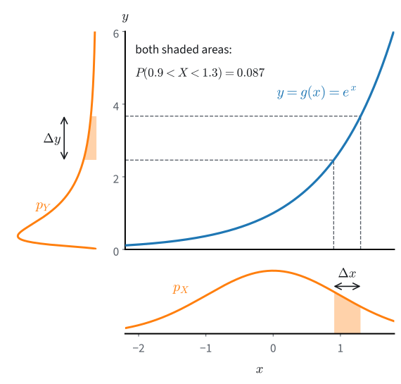
The obvious guess, \(p_Y(y)=p_X(g^{-1}(y))\), is wrong, and the dart already shows why. Its distance is sampled as \(R=\sqrt U\) with \(U\) uniform on \([0,1]\), and this map turns the flat density of \(U\) into the density \(2r\), which is not flat. The probability in a short interval must survive the map. An interval of width \(\Delta x\) at \(x\) carries probability about \(p_X(x)\,\Delta x\), and \(g\) sends it to an interval of width about \(\Delta y=|g'(x)|\,\Delta x\) at \(y=g(x)\), which must carry the same probability:
\[ p_Y(y)\,|g'(x)|\,\Delta x\approx p_X(x)\,\Delta x . \]
Where \(g\) stretches the line, the density must thin by the stretch factor \(|g'(x)|\); where \(g\) compresses, the density must rise. Figure 36.2.5 shows the two equal areas for \(Y=e^X\).
Proposition (change of variables in one dimension). Let \(X\) have a density \(p_X\) that is continuous on an open interval \(I\) with \(P(X\in I)=1\), and let \(g:I\to\mathbb{R}\) be continuously differentiable with \(g'\ne0\) on \(I\), so that \(g\) is strictly monotone and one-to-one. Then \(Y=g(X)\) has the density
\[ p_Y(y) = p_X\!\big(g^{-1}(y)\big)\,\left|\frac{d g^{-1}}{dy}(y)\right| \tag{36.2.13}\]
on the interval \(g(I)\), and \(0\) outside it.
Proof. Let \(g\) be increasing. Then \(g(X)\le y\) exactly when \(X\le g^{-1}(y)\), so the c.d.f.s satisfy \(F_Y(y)=F_X(g^{-1}(y))\) for \(y\) in \(g(I)\). Differentiating with the chain rule and Equation 36.1.5 gives \(p_Y(y)=p_X(g^{-1}(y))\,\frac{dg^{-1}}{dy}(y)\). If \(g\) is decreasing, then \(g(X)\le y\) exactly when \(X\ge g^{-1}(y)\), so \(F_Y(y)=1-F_X(g^{-1}(y))\). Its derivative carries a minus sign, which cancels the negative sign of \(dg^{-1}/dy\); the absolute value covers both cases. In either case \(F_Y\) is continuously differentiable on \(g(I)\), which carries all the probability, so by the fundamental theorem of calculus its derivative is a density of \(Y\). \(\blacksquare\)
The new density is the old one, read at the point that maps to \(y\), times the local compression of the inverse map. Since \(dg^{-1}/dy=1/g'(x)\) at \(x=g^{-1}(y)\), this is the factor \(1/|g'(x)|\) of the stretching argument.
Inverse-transform sampling is a change of variables, and the rule recovers the dart’s density from its sampler. Take \(X=U\), uniform on \(I=(0,1)\), and \(g(u)=\sqrt u\), so \(g^{-1}(r)=r^2\) and \(|dg^{-1}/dr|=2r\). The rule gives \(p_R(r)=1\cdot 2r\), the density of the dart’s distance.
When \(g\) is not one-to-one, several points map to the same \(y\), and their contributions add:
\[ p_Y(y)=\sum_{x:\,g(x)=y}\frac{p_X(x)}{|g'(x)|}, \]
for values \(y\) with finitely many preimages, each with \(g'(x)\ne0\). For \(Y=X^2\) and \(y>0\), the two preimages \(\pm\sqrt y\) have \(|g'|=2\sqrt y\), so \(p_Y(y)=[p_X(\sqrt y)+p_X(-\sqrt y)]/(2\sqrt y)\). The hypothesis \(g'\ne0\) matters. The ReLU has \(g'=0\) on the whole half-line \((-\infty,0)\), which it collapses to the single point \(0\), and the result is an atom rather than a density (Exercise 2).
As a worked example, let \(X\sim\mathcal N(0,1)\) have the standard normal density \(p_X(x)=e^{-x^2/2}/\sqrt{2\pi}\), and let \(Y=e^X\). Then \(g^{-1}(y)=\log y\) and \(|dg^{-1}/dy| = 1/y\) for \(y>0\), and the rule gives the log-normal density
\[ p_Y(y) = \frac{1}{y\sqrt{2\pi}}\,\exp\!\Big(-\tfrac12(\log y)^2\Big), \qquad y>0. \]
The factor \(1/y\) is the change-of-variables correction. Setting the derivative of \(\log p_Y(y)=-\log y-\tfrac12(\log y)^2+\textrm{const}\) to zero gives \(\log y=-1\), so the density peaks at \(y=e^{-1}\approx0.368\). The naive guess \(p_X(\log y)\) peaks at \(y=1\), and it is not even a density. Substituting \(y=e^x\), its total area is \(\int p_X(x)\,e^x\,dx=\mathbb{E}[e^X]=e^{1/2}\approx1.65\) (complete the square, \(x-x^2/2=\tfrac12-\tfrac12(x-1)^2\)).
The same computation gives the moments \(\mathbb{E}[Y^k]=\mathbb{E}[e^{kX}]=e^{k^2/2}\), all finite. Yet the tail \(P(Y>t)=P(X>\log t)\) decays more slowly than any exponential in \(t\). The log-normal is therefore heavy-tailed, although, unlike the Cauchy distribution, it has every moment.
The cell draws a histogram of \(10^5\) samples of \(e^X\) over both candidates. The naive curve must enclose \(0.65\) too much area; it is worth guessing where the excess sits before looking.
y = np.exp(rng.standard_normal(10**5))                 # Y = e^X
edges = np.linspace(0, 5, 101)
mids = (edges[:-1] + edges[1:]) / 2
hist = np.histogram(y, edges)[0] / (len(y) * (edges[1] - edges[0]))
p_X = lambda x: np.exp(-x**2 / 2) / np.sqrt(2 * np.pi)
d2l.plot(mids, [hist, p_X(np.log(mids)) / mids, p_X(np.log(mids))],
         'y', 'p(y)', figsize=(5, 3),
         legend=['histogram of exp(X)', 'log-normal', 'naive p_X(log y)'])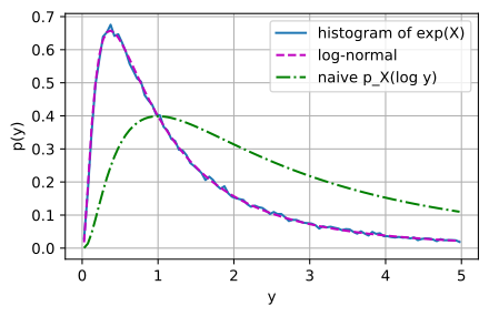
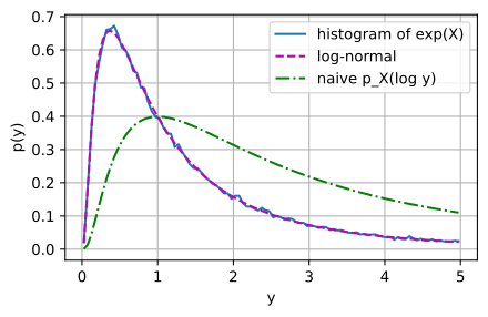
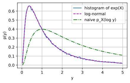
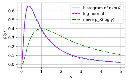
The histogram follows the log-normal curve up to sampling noise, with its peak well left of \(y=1\), near \(e^{-1}\). The naive curve peaks in the wrong place. It is the true density times \(y\), so it lies below the data for \(y<1\) and above it for \(y>1\), by a factor that grows into the tail.
36.2.3.2 The Multivariate Rule
In several dimensions, a map stretches areas and volumes rather than lengths, and the stretch factor becomes a determinant. The smallest case is a linear map. Let \(\mathbf Y=\mathbf A\mathbf X\) with \(\mathbf A=\operatorname{diag}(2,3)\). A unit square becomes a \(2\times3\) rectangle, which must carry the same probability as the square, spread over area \(6=\det\mathbf A\). So the density of \(\mathbf Y\) is one sixth of the density of \(\mathbf X\) at the corresponding point, \(p_{\mathbf Y}(\mathbf y)=p_{\mathbf X}(\mathbf A^{-1}\mathbf y)/6\).
For a nonlinear map, the stretch varies from point to point, and the change of variables theorem for integrals accounts for it (Section 34.6). Let \(g\) be a continuously differentiable bijection between two regions of \(\mathbb{R}^n\), with continuously differentiable inverse, and write \(J_{g^{-1}}\) for the Jacobian matrix of partial derivatives of the inverse. Locally, \(g^{-1}\) scales volume by \(|\det J_{g^{-1}}|\), and substituting \(\mathbf x=g^{-1}(\mathbf y)\) in an integral over the preimage of a region \(\mathcal D\) gives
\[ \int_{g^{-1}(\mathcal D)} f(\mathbf x)\,d\mathbf x=\int_{\mathcal D} f\bigl(g^{-1}(\mathbf y)\bigr)\,\bigl|\det J_{g^{-1}}(\mathbf y)\bigr|\,d\mathbf y . \]
Now let \(\mathbf Y=g(\mathbf X)\). The event \(\mathbf Y\in\mathcal D\) is the event \(\mathbf X\in g^{-1}(\mathcal D)\), so the theorem with \(f=p_{\mathbf X}\) reads
\[ P(\mathbf Y\in \mathcal D)=\int_{g^{-1}(\mathcal D)}p_{\mathbf X}(\mathbf x)\,d\mathbf x =\int_{\mathcal D} p_{\mathbf X}\bigl(g^{-1}(\mathbf y)\bigr)\,\bigl|\det J_{g^{-1}}(\mathbf y)\bigr|\,d\mathbf y . \]
The integrand on the right is therefore the density of \(\mathbf Y\):
\[ \begin{aligned} p_{\mathbf Y}(\mathbf y) &= p_{\mathbf X}\!\big(g^{-1}(\mathbf y)\big)\,\big|\det J_{g^{-1}}(\mathbf y)\big|, \\ \textrm{equivalently}\qquad \log p_{\mathbf Y}(\mathbf y) &= \log p_{\mathbf X}(\mathbf x) - \log\big|\det J_{g}(\mathbf x)\big| \quad\textrm{at }\mathbf x = g^{-1}(\mathbf y). \end{aligned} \tag{36.2.14}\]
The second form uses \(J_{g^{-1}}(\mathbf y)=J_g(\mathbf x)^{-1}\). Passing a sample through \(g\) subtracts the log of the local volume stretch from its log-density. Because \(\log|\det(J_2 J_1)| = \log|\det J_1| + \log|\det J_2|\), a composition of maps subtracts the sum of their log-determinants. This is how normalizing flows compute exact likelihoods: they stack invertible layers whose log-determinants are cheap (Rezende and Mohamed 2015), and Section 38.2.3 builds one whose layers are the steps of a differential equation. Exercise 6 builds a coupling layer.
The dart gives a last example. Describe its position in polar coordinates, the distance \(R\) and the angle \(\Theta\), with \((x,y)=(r\cos\theta,r\sin\theta)\). The Jacobian determinant of this map from \((r,\theta)\) to \((x,y)\) is \(\cos\theta\cdot r\cos\theta-(-r\sin\theta)\sin\theta=r\), so the rule gives
\[ p_{R,\Theta}(r,\theta)=\frac1\pi\cdot r=2r\cdot\frac{1}{2\pi}, \qquad 0\le r\le1,\ 0\le\theta<2\pi . \]
The joint density factorizes. The angle is uniform on \([0,2\pi)\), the distance has the density \(2r\) once more, now from a Jacobian, and the two are independent. In Cartesian coordinates the dart’s \(X\) and \(Y\) were dependent; in the right coordinates the same dart is described by two independent variables.
The section leaves a question about averages. We know the variance of an average of \(n\) independent draws, \(\sigma^2/n\) Equation 36.2.10, but not its distribution. Chebyshev’s inequality (Section 36.1) turns the variance into a bound, \(\sigma^2/(n\epsilon^2)\), on the chance that the average errs by \(\epsilon\) or more, and for bounded or Gaussian draws this is far too pessimistic: the chance falls exponentially fast in \(n\). Which distribution an average approaches is settled in Section 36.3.2.3, and the exponential rate in Section 36.9. Before either, we need densities other than the dart’s.
36.2.4 Summary
Marginals come from integrating out, and conditionals from slicing the joint density along a thin strip. The conditional mean is the best squared-error predictor, and the law of total variance splits a variance into the part that the conditioning variable explains and the part it cannot. Covariance and correlation measure a linear trend, not dependence in general, and the average of \(n\) independent draws with finite variance has variance \(\sigma^2/n\). A smooth invertible map changes a density by the factor of its local stretch, the absolute Jacobian determinant. The dart shows all of it: its coordinates are dependent and uncorrelated, and in polar coordinates they become two independent variables.
36.2.5 Exercises
[code] Classes missing from a minibatch. A minibatch holds \(B\) labels drawn independently and uniformly from \(K\) classes. Let \(M\) be the number of classes that do not appear in it, and write \(M = \sum_{k=1}^K I_k\), where \(I_k = 1\) if class \(k\) is missing and \(I_k = 0\) otherwise.
- Compute \(\mathbb{E}[M]\) with linearity Equation 36.1.7, and evaluate it for \(K = 1000\) and \(B = 256\).
- Compute \(\textrm{Cov}(I_j, I_k)\) for \(j \neq k\). Are the indicators independent?
- Extend the variance-of-a-sum rule Equation 36.2.9 to \(K\) terms, and compute the standard deviation of \(M\) for \(K = 1000\) and \(B = 256\). Compare it with the value that independent indicators would give, and check both against \(10^4\) simulated minibatches. How can covariances as small as those in (b) change the answer this much?
Uncorrelated but dependent. Whitening, for example with the principal components of Section 33.5, makes coordinates uncorrelated. The following pair has Gaussian coordinates and zero covariance. Let \(X \sim \mathcal{N}(0, 1)\), let \(S\) be a random sign independent of \(X\) with \(P(S = 1) = P(S = -1) = \tfrac12\), and let \(Y = SX\).
- Show that \(Y \sim \mathcal{N}(0, 1)\) by computing its c.d.f., and that \(\textrm{Cov}(X, Y) = 0\).
- Compare \(P(|X| \le 1, |Y| \le 1)\) with \(P(|X| \le 1)\,P(|Y| \le 1)\). Are \(X\) and \(Y\) independent?
- Show that \(X + Y\) has an atom at \(0\), so that \(X + Y\) is not Gaussian. With probability one the point \((X, Y)\) lies on one of the two lines \(y = \pm x\), and a double integral over a line is zero, because a line has no area. Conclude that the pair \((X, Y)\) has no joint density, although each coordinate has one.
Averaging correlated estimates. The text derives \(\textrm{Var}(\bar X_n) = \sigma^2/n\) for independent draws. Averages of dependent estimates behave differently.
Let \(Y_1, \ldots, Y_n\) each have variance \(\sigma^2\), with correlation \(\rho\) between every pair, as the predictions of \(n\) ensemble members trained on the same data might. Show that
\[\textrm{Var}\Bigl(\frac1n\sum_{i=1}^n Y_i\Bigr) = \sigma^2\Bigl(\rho + \frac{1-\rho}{n}\Bigr). \tag{36.2.15}\]
What does averaging achieve as \(n \to \infty\)?
Use \(\mathbf{a}^\top \boldsymbol\Sigma\, \mathbf{a} \ge 0\) for the covariance matrix \(\boldsymbol\Sigma\) of \(Y_1, \ldots, Y_n\) to show that \(\rho \ge -1/(n-1)\). Give variables that attain this bound.
[code] Sigmoid of a Gaussian. Let \(X \sim \mathcal{N}(0, s^2)\) be the pre-activation of a sigmoid unit, and let \(Y = \operatorname{sigmoid}(X)\), whose inverse is \(\operatorname{logit}(y) = \log\bigl(y/(1-y)\bigr)\).
- Use Equation 36.2.13 to find the density \(p_Y\) on \((0, 1)\).
- For which \(s\) is \(y = \tfrac12\) a local minimum of \(p_Y\)? Writing \(\log p_Y\) as a function of \(z = \operatorname{logit}(y)\) simplifies the computation.
- Modify the
#random-variables-change-of-variablescell to compare a histogram of \(Y\) with \(p_Y\) for \(s \in \{1, \sqrt{2}, 3\}\). What does the histogram at \(s = 3\) imply for the derivative \(\operatorname{sigmoid}'(X) = Y(1 - Y)\), through which backpropagation passes the gradient of these units?
Explained variance. ● A regression model \(h\) predicts a target \(X\) from an input \(Y\). The fraction of the variance that it explains is \(R^2 = 1 - \mathbb{E}\bigl[(X - h(Y))^2\bigr]/\textrm{Var}(X)\).
- Use Equation 36.2.6 and the law of total variance Equation 36.2.5 to show that every predictor has \(R^2 \le \textrm{Var}\bigl(\mathbb{E}[X \mid Y]\bigr)/\textrm{Var}(X)\). Evaluate this ceiling for the two-component mixture of the text, predicting \(X\) from the label \(Z\), and for the dart, predicting \(X\) from \(Y\).
- Given the input, the target is \(-1\) or \(+1\) with probability \(\tfrac12\) each. Which prediction minimizes the expected squared error, and how often does the target take that value? Which predictions minimize the expected absolute error \(\mathbb{E}\bigl[|X - h(Y)|\bigr]\)?
[code] Affine coupling layer and Box–Muller. ● Normalizing flows stack invertible maps whose log-determinants in Equation 36.2.14 are cheap to compute. The affine coupling layer of RealNVP (Dinh et al. 2017) maps \(\mathbf{x} \in \mathbb{R}^2\) to
\[y_1 = x_1, \qquad y_2 = x_2\, e^{s(x_1)} + t(x_1), \tag{36.2.16}\]
where \(s\) and \(t\) are arbitrary functions, for example small neural networks.
- Write down the inverse map and the Jacobian \(J_g(\mathbf{x})\). Show that \(\log|\det J_g(\mathbf{x})| = s(x_1)\), however complicated \(s\) and \(t\) are.
- Let \(X_1\) and \(X_2\) be independent standard normal variables, and take \(s(x_1) = \tanh(x_1)\) and \(t(x_1) = x_1^2/2\). Use Equation 36.2.14 to write \(\log p_{\mathbf{Y}}(\mathbf{y})\) in closed form. With NumPy, evaluate \(p_{\mathbf{Y}}\) on a grid over \([-6, 6] \times [-12, 24]\) with spacing \(0.02\) and check that its Riemann sum is close to \(1\). Check the log-determinant against the determinant of a finite-difference Jacobian at a few random points.
- The first coordinate passes through the layer unchanged. What is the distribution of \(Y_1\), whatever \(s\) and \(t\) are? How must a second coupling layer be arranged so that the composition can change both marginals, and what is the log-determinant of the composition?
- Flows can also run from uniform noise to Gaussians. Let \(U_1, U_2\) be independent and uniform on \((0, 1)\), and set \(R = \sqrt{-2\log U_1}\), \(\Theta = 2\pi U_2\), and \((Z_1, Z_2) = (R\cos\Theta, R\sin\Theta)\). Find the density of \(R\) with the one-dimensional rule, then the joint density of \((R, \Theta)\), and change to Cartesian coordinates with the polar Jacobian of the text to show that \(Z_1\) and \(Z_2\) are independent standard normal variables. This is the Box–Muller method. Check with \(10^5\) samples that the sample covariance matrix of \((Z_1, Z_2)\) is close to the identity.