from d2l import torch as d2l
import torch3.3 The Base Classification Model
Classification models require a validation step that reports both loss and accuracy, together with an optimizer. We implement these shared operations in a Classifier base class extending the d2l.Module introduced in Section 2.2. A subclass then supplies the model-specific forward method and, when needed, a loss other than cross-entropy.
from d2l import tensorflow as d2l
import tensorflow as tf
from d2l import jax as d2l
from jax import numpy as jnp
import optaxfrom d2l import mxnet as d2l
from mxnet import autograd, np, npx, gluon
npx.set_np()3.3.1 The Classifier Class
The Classifier class reports loss and accuracy for each validation batch. These curves are monitoring diagnostics: an unweighted average of batch means differs from the exact dataset metric when the final batch is smaller. Final evaluation should instead sum per-example losses and correct indicators and divide by the total number of examples.
The _report_val method mirrors validation_step but accepts a precomputed y_hat, so the compiled validation graph (see Section 2.4) only needs to run the forward pass once.
NNX modules own their parameters and other state. The compiled trainer can therefore call the model directly, while NNX tracks updates such as BatchNorm running statistics automatically. The validation step returns its two metrics to the trainer, which records them outside the compiled computation.
class Classifier(d2l.Module):
    """The base class of classification models."""
    def validation_step(self, batch):
        Y_hat = self(*batch[:-1])
        self.plot('loss', self.loss(Y_hat, batch[-1]), train=False)
        self.plot('acc', self.accuracy(Y_hat, batch[-1]), train=False)

    def _report_val(self, y_hat, batch):
        self.plot('loss', self.loss(y_hat, batch[-1]), train=False)
        self.plot('acc', self.accuracy(y_hat, batch[-1]), train=False)
class Classifier(d2l.Module):
"""The base class of classification models."""
def validation_step(self, batch):
Y_hat = self(*batch[:-1])
self.plot('loss', self.loss(Y_hat, batch[-1]), train=False)
self.plot('acc', self.accuracy(Y_hat, batch[-1]), train=False)
def _report_val(self, y_hat, batch):
self.plot('loss', self.loss(y_hat, batch[-1]), train=False)
self.plot('acc', self.accuracy(y_hat, batch[-1]), train=False)class Classifier(d2l.Module):
"""The base class of classification models."""
def validation_step(self, batch):
Y_hat = self(*batch[:-1])
return self.loss(Y_hat, batch[-1]), self.accuracy(Y_hat, batch[-1])class Classifier(d2l.Module):
"""The base class of classification models."""
def validation_step(self, batch):
Y_hat = self(*batch[:-1])
self.plot('loss', self.loss(Y_hat, batch[-1]), train=False)
self.plot('acc', self.accuracy(Y_hat, batch[-1]), train=False)
def _report_val(self, y_hat, batch):
self.plot('loss', self.loss(y_hat, batch[-1]), train=False)
self.plot('acc', self.accuracy(y_hat, batch[-1]), train=False)By default we use a stochastic gradient descent optimizer operating on minibatches, just as we did in the context of linear regression. configure_optimizers is a hook: Trainer calls it once at the start of training (see Section 2.2), and it returns the optimizer object that Trainer then uses to update the parameters after each backward pass. We install it on d2l.Module rather than Classifier because regression models use the same default; a subclass can still override it (later chapters do exactly that) to switch optimizers.
@d2l.add_to_class(d2l.Module)
def configure_optimizers(self):
return torch.optim.SGD(self.parameters(), lr=self.lr)@d2l.add_to_class(d2l.Module)
def configure_optimizers(self):
return tf.keras.optimizers.SGD(float(self.lr))@d2l.add_to_class(d2l.Module)
def configure_optimizers(self):
return optax.sgd(self.lr)@d2l.add_to_class(d2l.Module)
def configure_optimizers(self):
params = self.parameters()
if isinstance(params, list):
return d2l.SGD(params, self.lr)
return gluon.Trainer(params, 'sgd', {'learning_rate': self.lr})3.3.2 Accuracy
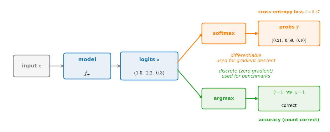
A classifier uses the same score vector \(\mathbf{o}\in\mathbb{R}^q\) for training and evaluation in different ways (Figure 3.3.1). During training, softmax converts the scores to probabilities and cross-entropy provides a smooth loss for gradient descent. The loss distinguishes, for example, correct-class probabilities of \(0.51\) and \(0.99\) even though both produce the same hard decision. During evaluation, \(\arg\max\) converts the scores to a class \(\hat{y}\), and accuracy records whether it matches the label. Accuracy is discrete and has zero gradient almost everywhere, so it is unsuitable as the direct training objective. Whether it is an appropriate deployment metric depends on the costs of different errors and on how predictions are used.
We therefore report both quantities. The loss measures probability quality and supplies the optimization objective; accuracy measures hard decisions. A decreasing loss with unchanged accuracy can indicate increasing margins or changing calibration rather than an implementation error.
Many applications require a hard decision. Given the predicted distribution y_hat, we select its highest-probability class. An email system, for example, may estimate probabilities internally but ultimately assign each message to one folder. Accuracy is the fraction of selected classes that match the labels y.
Accuracy is computed as follows. First, if y_hat is a matrix, we assume that the second dimension stores prediction scores for each class. We use argmax to obtain the predicted class by the index for the largest entry in each row. Then we compare the predicted class with the ground truth y elementwise. Since the equality operator == is sensitive to data types, we cast the predicted classes (preds) to y’s dtype. The result is a tensor containing entries of 0 (false) and 1 (true). Averaging the 0/1 entries yields the fraction correct (or, with averaged=False, the raw 0/1 vector).
@d2l.add_to_class(Classifier)
def accuracy(self, Y_hat, Y, averaged=True):
    """Compute the fraction of correct predictions."""
    Y_hat = d2l.reshape(Y_hat, (-1, Y_hat.shape[-1]))
    preds = d2l.astype(d2l.argmax(Y_hat, axis=1), Y.dtype)
    compare = d2l.astype(preds == d2l.reshape(Y, (-1,)), d2l.float32)
return d2l.reduce_mean(compare) if averaged else compare@d2l.add_to_class(Classifier)
def accuracy(self, Y_hat, Y, averaged=True):
"""Compute the fraction of correct predictions."""
Y_hat = d2l.reshape(Y_hat, (-1, Y_hat.shape[-1]))
preds = d2l.astype(d2l.argmax(Y_hat, axis=1), Y.dtype)
compare = d2l.astype(preds == d2l.reshape(Y, (-1,)), d2l.float32)
return d2l.reduce_mean(compare) if averaged else compare@d2l.add_to_class(Classifier)
def accuracy(self, Y_hat, Y, averaged=True):
"""Compute the fraction of correct predictions."""
Y_hat = d2l.reshape(Y_hat, (-1, Y_hat.shape[-1]))
preds = d2l.astype(d2l.argmax(Y_hat, axis=1), Y.dtype)
compare = d2l.astype(preds == d2l.reshape(Y, (-1,)), d2l.float32)
return d2l.reduce_mean(compare) if averaged else compareThe NNX version receives the precomputed scores just like the other frameworks. The surrounding validation step is compiled, so this small metric does not need its own jit decorator.
@d2l.add_to_class(Classifier)
def accuracy(self, Y_hat, Y, averaged=True):
    """Compute the fraction of correct predictions."""
    Y_hat = d2l.reshape(Y_hat, (-1, Y_hat.shape[-1]))
    preds = d2l.astype(d2l.argmax(Y_hat, axis=1), Y.dtype)
    compare = d2l.astype(preds == d2l.reshape(Y, (-1,)), d2l.float32)
return d2l.reduce_mean(compare) if averaged else compareMXNet’s gluon.Block.collect_params only finds parameters declared through Gluon’s Parameter machinery, so it misses the bare np.ndarray attributes that the from-scratch implementations in this book use. We extend d2l.Module with a fallback get_scratch_params that walks attributes recursively, and a parameters method that returns Gluon’s params when present and the scratch params otherwise. This fallback is specific to Gluon’s parameter API.
@d2l.add_to_class(d2l.Module)
def get_scratch_params(self):
    # collect_params() only finds Parameters declared via Gluon's Parameter
    # API. For from-scratch models that store weights as bare np.ndarrays, we
    # walk the object's attributes recursively and gather those instead.
    params = []
    for attr in dir(self):
        a = getattr(self, attr)
        if isinstance(a, np.ndarray):
            params.append(a)
        if isinstance(a, d2l.Module):
            params.extend(a.get_scratch_params())
    return params

@d2l.add_to_class(d2l.Module)
def parameters(self):
    # Return the Gluon ParameterDict when the model uses Gluon layers; fall
    # back to the bare-array scan for from-scratch implementations.
    params = self.collect_params()
    return params if isinstance(params, dict) and len(
        params.keys()) else self.get_scratch_params()
3.3.3 Beyond Accuracy
Accuracy treats every example, and every kind of mistake, as equally important. Once classes are imbalanced, that assumption fails in a way that can make accuracy actively misleading. Consider screening for a disease that affects 1% of the population. A classifier that ignores its input and always predicts healthy is right 99% of the time, so its accuracy is 0.99, but it finds not a single sick patient. The counts make this concrete:
n, sick = 100_000, 1_000            # 1% of the population carries the disease
tp, fp, fn = 0, 0, sick             # "always predict healthy" never fires
accuracy = 1 - (fp + fn) / n
recall = tp / sick                  # fraction of sick patients found
accuracy, recall
(0.99, 0.0)The numbers that expose the failure come from breaking the counts down by what was predicted and what was true. For a binary problem there are four cases, which we arrange in a \(2\times2\) table: true positives (TP, predicted positive, was positive), false positives (FP, predicted positive, was negative), false negatives (FN, predicted negative, was positive), and true negatives (TN). Two ratios summarize the two failure modes:
\[\textrm{precision} = \frac{\textrm{TP}}{\textrm{TP} + \textrm{FP}}, \qquad \textrm{recall} = \frac{\textrm{TP}}{\textrm{TP} + \textrm{FN}}. \tag{3.3.1}\]
Precision asks: of the examples we flagged, how many were real? Recall asks: of the real positives, how many did we find? The always-healthy classifier above has recall \(0\) (and its precision is undefined, since it never flags anyone), which tells the true story that the 99% accuracy conceals. When a single summary number is needed, the conventional compromise is the F1 score, the harmonic mean \(2\,\textrm{PR}/(\textrm{P}+\textrm{R})\) of precision and recall, which is high only when both are.
For \(q\) classes the same bookkeeping becomes a \(q \times q\) confusion matrix \(C\) with entries
\[C_{ij} = \sum_{k=1}^n \mathbf{1}(\hat{y}^{(k)} = i)\, \mathbf{1}(y^{(k)} = j), \tag{3.3.2}\]
where \(y^{(k)}\) and \(\hat{y}^{(k)}\) denote the true and predicted class of example \(k\): entry \((i, j)\) counts the examples of true class \(j\) that the model predicted as class \(i\), so the diagonal holds the correct decisions and every off-diagonal cell isolates one specific kind of error. A confusion matrix is one useful classification diagnostic; a single accuracy number is its normalized trace (the fraction on the diagonal). We will meet it twice more in this chapter: in Section 3.4 we compute one for our trained Fashion-MNIST classifier to see which classes it confuses, and in Section 3.7 the same matrix becomes the key computational object for correcting label shift.
3.3.4 Summary
The Classifier class adds two things to d2l.Module: an overridden validation_step that logs both the loss and the accuracy, and a default configure_optimizers that returns a minibatch SGD optimizer. Because of this, every classification model in the rest of the book can subclass Classifier and supply only its forward pass (and a custom loss, where the default cross-entropy will not do), inheriting the whole training and evaluation loop. Accuracy itself is the fraction of examples whose predicted class matches the true label, where the predicted class is the \(\arg\max\) of the score vector. It is a discrete metric and so cannot serve as a training objective, but it is commonly reported in benchmarks and should be watched alongside the loss when all mistakes have comparable costs. On imbalanced or cost-sensitive problems, accuracy alone can badly mislead; precision, recall, and the confusion matrix break the errors down by kind, and the confusion matrix in particular will return twice more in this chapter.
3.3.5 Exercises
Batch-mean validation loss. The \(n\) validation examples are split into batches of size \(b\), except the last batch, whose size is \(r\) with \(0 < r \leq b\). Let \(L_\textrm{v}\) be the validation loss, the average of the per-example losses over all \(n\) examples. Let \(\bar{L}_\textrm{v}\) be the unweighted average of the per-batch mean losses that
validation_stepcomputes, and let \(l_\textrm{v}^\textrm{last}\) be the mean loss of the last batch.- Express \(L_\textrm{v}\) in terms of \(\bar{L}_\textrm{v}\), \(l_\textrm{v}^\textrm{last}\), \(n\), \(b\), and \(r\).
- Treat the validation examples as i.i.d. draws from the data distribution. Show that \(L_\textrm{v}\) and \(\bar{L}_\textrm{v}\) are both unbiased estimates of the risk, so that \(E[L_\textrm{v}] = E[\bar{L}_\textrm{v}]\).
- Compare the variances of the two estimates and explain why \(L_\textrm{v}\) is preferable for a final evaluation.
Optimal decisions and rejection. In a multiclass problem, let \(l(y, y')\) be the penalty for predicting \(y'\) when the true class is \(y\), and let \(p(y \mid x)\) be the probability of class \(y\) given the input \(x\).
- Write the expected loss of predicting \(y'\) in terms of \(l\) and \(p(y \mid x)\), and state the rule that selects the optimal \(y'\).
- Let a correct guess cost \(0\) and a wrong guess cost \(\lambda_s\), and allow the classifier to abstain instead of guessing, at a fixed cost \(\lambda_r < \lambda_s\). Derive the threshold on the top-class probability above which guessing beats abstaining.
- In medical diagnosis, deferring to a specialist is cheap relative to a misdiagnosis, say \(\lambda_r/\lambda_s = 0.05\). Compute the threshold and state what the classifier should do with a prediction at \(0.9\) confidence. Then describe a case in which reporting the full distribution \(p(y \mid x)\) serves the physician better than either guessing or abstaining.
Adapted from Kevin Murphy, Probabilistic Machine Learning: An Introduction, Exercise 5.1.
Loss at equal accuracy. Two classifiers \(A\) and \(B\) both achieve 90% accuracy on a ten-class test set. On every example that \(A\) classifies correctly, it assigns probability \(0.91\) to the correct class. On every example that \(B\) classifies correctly, it assigns \(0.51\).
- Compute the average cross-entropy loss of each classifier on its correctly classified examples. Why would knowing only that \(B\)’s average correct-class probability is \(0.51\) not have sufficed to compute \(B\)’s loss?
- Explain why these numbers do not decide which classifier is safer to deploy, and list the further information about the two classifiers you would need.
- Temperature scaling (exercise 8 of Section 3.1) divides \(B\)’s logits by \(T > 0\) and leaves every one of its decisions unchanged. Assume that on every example the largest logit of \(B\) is unique. Show that as \(T \to 0\) the cross-entropy of \(B\) tends to \(0\) on the correctly classified examples and to \(\infty\) on the misclassified ones. What does this imply about comparing classifiers by loss alone?
[code] Top-\(k\) accuracy. Generalize
accuracyto top-\(k\) accuracy, which counts a prediction as correct when the true class is among the \(k\) highest-scoring classes.- Add a
kargument toaccuracy, replacing the singleargmaxby the indices of the \(k\) largest scores, and check that the result equals \(1\) whenkequals the number of classes. - Why is top-5 accuracy a standard companion to top-1 on benchmarks with many fine-grained classes?
- Add a
Class-weighted loss. In the disease-screening example of Section 3.3.3, missing a sick patient costs much more than a false alarm. Give each class \(j\) a weight \(w_j > 0\) and train \(f\) on the class-weighted empirical risk
\[\frac{1}{n} \sum_{i=1}^n w_{y_i}\, l(f(\mathbf{x}_i), y_i),\]
where \(l\) is the cross-entropy loss and \(y_i\) is the class of example \(i\). This is the weighted empirical risk minimization Equation 3.7.2 of Section 3.7 with \(\beta_i = w_{y_i}\).
- Let the training examples be drawn with class prior \(p(y)\) and class-conditional densities \(p(\mathbf{x} \mid y)\). Show that the expected class-weighted loss is proportional to the expected unweighted loss under the distribution with the same class-conditionals and class prior proportional to \(w_y\, p(y)\). Name the change to the training data, rather than to the loss, that has the same effect.
- Fix an input \(\mathbf{x}\) with class probabilities \(p(j \mid \mathbf{x})\), and suppose the model can output any distribution \(\hat{\mathbf{y}}\). Show that the expected weighted loss \[-\sum_j w_j\, p(j \mid \mathbf{x}) \log \hat{y}_j \tag{3.3.3}\] is minimized by \(\hat{y}_j \propto w_j\, p(j \mid \mathbf{x})\).
- For the two classes healthy and sick, find the threshold on \(p(\textrm{sick} \mid \mathbf{x})\) above which the \(\arg\max\) of this \(\hat{\mathbf{y}}\) is sick. Explain why choosing \(w_\textrm{sick} > w_\textrm{healthy}\) raises recall, and what it does to the number of false positives.
[code] ROC curves. A binary classifier that outputs a score \(s \in (0, 1)\) for the positive class can be thresholded at any \(\tau \in [0, 1]\), not just \(\frac{1}{2}\): predict positive whenever \(s > \tau\). The receiver operating characteristic (ROC) curve plots the true-positive rate (recall) against the false-positive rate \(\textrm{FP}/(\textrm{FP}+\textrm{TN})\) as \(\tau\) sweeps from \(1\) down to \(0\). Simulate \(1000\) positive and \(1000\) negative examples with scores \(s = \sigma(z)\), where \(\sigma\) is the sigmoid of Equation 3.1.3, \(z \sim \mathcal{N}(\mu, 1)\) for positives, and \(z \sim \mathcal{N}(0, 1)\) for negatives.
- Compute and plot the ROC curve for \(\mu \in \{0, 1, 2\}\), and state which points of the plot the endpoints \(\tau = 1\) and \(\tau = 0\) give.
- Show that a classifier whose scores are independent of the labels traces the diagonal in expectation.
[code] AUC as ranking probability. ● This problem uses the ROC curves and simulated scores of the previous problem.
- Show that, when no two scores tie, the area under the ROC curve equals the probability that a randomly chosen positive example receives a higher score than a randomly chosen negative one, which makes it a threshold-free summary of ranking quality.
- Compute this probability in closed form for the simulated scores and compare it with the trapezoidal area under each of the curves.