torch.set_float32_matmul_precision('high') # tf32 matmuls on tensor cores17.5 Likelihood, Weighting and the Design Space
For four sections we have trained networks by regression onto a per-example target and accepted the result because it worked: samples of the mixture land on its three modes with the right weights, and the garments of Section 17.3 look like garments. We have never asked what probability the model assigns to a data point, a density model’s first question and one the adversarial models of Chapter 16 could not answer. Is “predict the noise” maximum likelihood in disguise, and what negative log-likelihood does it give the mixture, whose true value is about 2.5 nats per point? And which of the choices made along the way (the target, the weight of each noise level, the schedule) matter?
Sohl-Dickstein et al. (2015) and Ho et al. (2020) derived the model as a latent-variable model whose latents are the noisy copies of a data point, with a lower bound on the log-likelihood that is a sum of noise regressions, one per noise level, each with its own weight; the loss of Section 17.2 sets every weight to one. Kingma and Gao (2023) showed that every diffusion objective, flow matching included, is the same integral over the log signal-to-noise ratio with its own weighting. The section ends with the design choices of Karras et al. (2022), noise levels as image scales, and four recipes on Fashion-MNIST.
17.5.1 The Likelihood Bound
Read backward, the chain of Section 17.2 is a generative model with \(T\) layers of latent variables, whose likelihood we can bound.
17.5.1.1 The Chain as a Latent-Variable Model
Step \(k\) of the forward chain shrinks the current point and adds noise, \(\mathbf{x}_k = \sqrt{1 - \beta_k}\, \mathbf{x}_{k-1} + \sqrt{\beta_k}\, \boldsymbol\epsilon_k\), and the steps compose into one Gaussian draw, \(\mathbf{x}_k = \alpha_k \mathbf{x}_0 + \sigma_k \boldsymbol\epsilon\) with \(\alpha_k^2 = \prod_{j \le k}(1 - \beta_j)\) and \(\sigma_k^2 = 1 - \alpha_k^2\): the VP path at the times \(t_k = k/T\). We write \(q\) for the distributions of this forward chain. The generative model runs it backward through learned Gaussian steps,
\[ p_{\boldsymbol\theta}(\mathbf{x}_{0:T}) = p(\mathbf{x}_T) \prod_{k=1}^{T} p_{\boldsymbol\theta}(\mathbf{x}_{k-1} \mid \mathbf{x}_k), \qquad p_{\boldsymbol\theta}(\mathbf{x}_{k-1} \mid \mathbf{x}_k) = \mathcal{N}\big(\boldsymbol\mu_{\boldsymbol\theta}(\mathbf{x}_k, k),\, \nu_k \mathbf{I}\big), \tag{17.5.1}\]
with \(p(\mathbf{x}_T) = \mathcal{N}(\mathbf{0}, \mathbf{I})\), a mean \(\boldsymbol\mu_{\boldsymbol\theta}\) computed by a network, and fixed variances \(\nu_k\) (\(\sigma_k\) remains the path’s noise scale). The density of \(\mathbf{x}_0\) integrates this joint over \(\mathbf{x}_{1:T}\), which we cannot compute, but any distribution over the latents gives a lower bound on it, the evidence lower bound (ELBO) of Section 41.5.5. The chain supplies one, the forward process itself. As an upper bound on the negative log-likelihood,
\[ -\log p_{\boldsymbol\theta}(\mathbf{x}_0) \le \mathbb{E}_{q(\mathbf{x}_{1:T} \mid \mathbf{x}_0)}\!\left[-\log \frac{p_{\boldsymbol\theta}(\mathbf{x}_{0:T})}{q(\mathbf{x}_{1:T} \mid \mathbf{x}_0)}\right] =: L(\mathbf{x}_0). \tag{17.5.2}\]
The gap is \(D_{\textrm{KL}}\big(q(\mathbf{x}_{1:T} \mid \mathbf{x}_0) \,\|\, p_{\boldsymbol\theta}(\mathbf{x}_{1:T} \mid \mathbf{x}_0)\big)\), so the bound is tight when the learned reverse chain, given \(\mathbf{x}_0\), retraces the forward chain.
Substituting the factorizations of both chains splits the bound into one term per step. With \(\mathbb{E}_q\) the expectation over \(q(\mathbf{x}_{1:T} \mid \mathbf{x}_0)\),
\[ \begin{aligned} L(\mathbf{x}_0) &= \mathbb{E}_q\Big[-\log p(\mathbf{x}_T) - \sum_{k=1}^{T} \log \frac{p_{\boldsymbol\theta}(\mathbf{x}_{k-1} \mid \mathbf{x}_k)}{q(\mathbf{x}_k \mid \mathbf{x}_{k-1})}\Big] \\ &= \mathbb{E}_q\Big[-\log p(\mathbf{x}_T) - \sum_{k=2}^{T} \log\Big(\frac{p_{\boldsymbol\theta}(\mathbf{x}_{k-1} \mid \mathbf{x}_k)}{q(\mathbf{x}_{k-1} \mid \mathbf{x}_k, \mathbf{x}_0)} \cdot \frac{q(\mathbf{x}_{k-1} \mid \mathbf{x}_0)}{q(\mathbf{x}_k \mid \mathbf{x}_0)}\Big) - \log \frac{p_{\boldsymbol\theta}(\mathbf{x}_0 \mid \mathbf{x}_1)}{q(\mathbf{x}_1 \mid \mathbf{x}_0)}\Big] \\ &= \mathbb{E}_q\Big[\log \frac{q(\mathbf{x}_T \mid \mathbf{x}_0)}{p(\mathbf{x}_T)} + \sum_{k=2}^{T} \log \frac{q(\mathbf{x}_{k-1} \mid \mathbf{x}_k, \mathbf{x}_0)}{p_{\boldsymbol\theta}(\mathbf{x}_{k-1} \mid \mathbf{x}_k)} - \log p_{\boldsymbol\theta}(\mathbf{x}_0 \mid \mathbf{x}_1)\Big]. \end{aligned} \tag{17.5.3}\]
The second line reverses each forward step by Bayes’ rule with \(\mathbf{x}_0\) held fixed: by the Markov property \(q(\mathbf{x}_k \mid \mathbf{x}_{k-1}) = q(\mathbf{x}_k \mid \mathbf{x}_{k-1}, \mathbf{x}_0)\), which equals \(q(\mathbf{x}_{k-1} \mid \mathbf{x}_k, \mathbf{x}_0)\, q(\mathbf{x}_k \mid \mathbf{x}_0) / q(\mathbf{x}_{k-1} \mid \mathbf{x}_0)\). In the third line the ratios of marginals telescope to \(q(\mathbf{x}_1 \mid \mathbf{x}_0) / q(\mathbf{x}_T \mid \mathbf{x}_0)\), whose numerator cancels the \(k = 1\) denominator. Each remaining logarithm is, in expectation, a divergence:
\[ L(\mathbf{x}_0) = \underbrace{D_{\textrm{KL}}\big(q(\mathbf{x}_T \mid \mathbf{x}_0) \,\|\, p(\mathbf{x}_T)\big)}_{L_T} + \sum_{k=2}^{T} \underbrace{\mathbb{E}_q\, D_{\textrm{KL}}\big(q(\mathbf{x}_{k-1} \mid \mathbf{x}_k, \mathbf{x}_0) \,\|\, p_{\boldsymbol\theta}(\mathbf{x}_{k-1} \mid \mathbf{x}_k)\big)}_{L_{k-1}} + \underbrace{\mathbb{E}_q\big[-\log p_{\boldsymbol\theta}(\mathbf{x}_0 \mid \mathbf{x}_1)\big]}_{L_0}. \tag{17.5.4}\]
The middle terms compare each learned step with the forward posterior \(q(\mathbf{x}_{k-1} \mid \mathbf{x}_k, \mathbf{x}_0)\), the reversal of step \(k\) for a known clean point. Conditioning on \(\mathbf{x}_0\) makes it computable: as a product of two Gaussians in \(\mathbf{x}_{k-1}\), the forward step and \(q(\mathbf{x}_{k-1} \mid \mathbf{x}_0)\), it is Gaussian (8 completes the square),
\[ q(\mathbf{x}_{k-1} \mid \mathbf{x}_k, \mathbf{x}_0) = \mathcal{N}\big(\tilde{\boldsymbol\mu}_k, \tilde\beta_k \mathbf{I}\big), \qquad \tilde{\boldsymbol\mu}_k = \frac{\alpha_{k-1}\beta_k}{\sigma_k^2}\, \mathbf{x}_0 + \frac{\sqrt{1 - \beta_k}\, \sigma_{k-1}^2}{\sigma_k^2}\, \mathbf{x}_k, \qquad \tilde\beta_k = \frac{\beta_k\, \sigma_{k-1}^2}{\sigma_k^2}. \tag{17.5.5}\]
The mean is a weighted average of where the clean point and the noisy point put \(\mathbf{x}_{k-1}\), and the variance is below the forward step’s \(\beta_k\): knowing both ends pins the middle down.
The smallest case shows the three kinds of terms. With one coordinate, \(T = 2\) and \(\beta_1 = \beta_2 = 1/2\), the prior term \(L_2\) compares the chain’s end \(\mathcal{N}(\alpha_2 x_0, \sigma_2^2)\) with \(\mathcal{N}(0, 1)\) and by the Gaussian formula Equation 16.1.8 equals \(x_0^2/8 + 0.019\): two large steps leave much of \(x_0\) behind. The denoising term \(L_1\) compares the learned step from \(x_2\) to \(x_1\) with the forward posterior, and the reconstruction term \(L_0\) scores the last step. At \(T = 1000\) the prior term is nearly zero and the denoising terms carry the training signal.
Averaged over the data, the bound is at least the cross-entropy \(\mathbb{E}_{p}[-\log p_{\boldsymbol\theta}(\mathbf{x}_0)] = H(p) + D_{\textrm{KL}}(p \,\|\, p_{\boldsymbol\theta})\): a model that drops a mode pays on every point of it.
17.5.1.2 From the Bound to Weighted Regression
Each denoising term compares two Gaussians whose variances do not depend on the network, so by Equation 16.1.8 only the distance between the means involves \(\boldsymbol\theta\):
\[ L_{k-1} = \mathbb{E}_q\Big[\frac{1}{2\nu_k} \big\|\tilde{\boldsymbol\mu}_k(\mathbf{x}_k, \mathbf{x}_0) - \boldsymbol\mu_{\boldsymbol\theta}(\mathbf{x}_k, k)\big\|^2\Big] + \textrm{const}, \tag{17.5.6}\]
where the constant vanishes for \(\nu_k = \tilde\beta_k\): each step asks the network for the mean of the forward posterior.
The network does not have to output that mean directly. Substituting \(\mathbf{x}_0 = (\mathbf{x}_k - \sigma_k \boldsymbol\epsilon)/\alpha_k\) into Equation 17.5.5 and using \(\sigma_k^2 = \beta_k + (1 - \beta_k)\sigma_{k-1}^2\), the coefficients of \(\mathbf{x}_k\) combine into \(1/\sqrt{1 - \beta_k}\) and the mean becomes
\[ \tilde{\boldsymbol\mu}_k = \frac{1}{\sqrt{1 - \beta_k}}\Big(\mathbf{x}_k - \frac{\beta_k}{\sigma_k}\, \boldsymbol\epsilon\Big). \tag{17.5.7}\]
Everything here but \(\boldsymbol\epsilon\) is known to a network that receives \(\mathbf{x}_k\) and \(k\), so we let it predict the noise and form its mean the same way,
\[ \boldsymbol\mu_{\boldsymbol\theta}(\mathbf{x}_k, k) = \frac{1}{\sqrt{1 - \beta_k}}\Big(\mathbf{x}_k - \frac{\beta_k}{\sigma_k}\, \hat{\boldsymbol\epsilon}_{\boldsymbol\theta}(\mathbf{x}_k, k)\Big), \tag{17.5.8}\]
and the difference of the two means is a multiple of the noise error:
\[ L_{k-1} = \mathbb{E}_{\mathbf{x}_0, \boldsymbol\epsilon}\Big[\frac{\beta_k^2}{2\nu_k (1 - \beta_k)\sigma_k^2}\, \big\|\boldsymbol\epsilon - \hat{\boldsymbol\epsilon}_{\boldsymbol\theta}(\alpha_k \mathbf{x}_0 + \sigma_k \boldsymbol\epsilon, k)\big\|^2\Big] + \textrm{const}. \tag{17.5.9}\]
Each term of the bound is the noise regression of Section 17.2 at one level, with a weight, for \(\nu_k = \tilde\beta_k\) equal to \(\beta_k / (2(1 - \beta_k)\sigma_{k-1}^2)\). Over step \(k\) the signal-to-noise ratio \(\alpha_k^2/\sigma_k^2\) falls by the factor \(\sigma_k^2 / ((1 - \beta_k)\sigma_{k-1}^2) = 1 + \beta_k/((1 - \beta_k)\sigma_{k-1}^2)\), so with \(\lambda_k = \log(\alpha_k^2/\sigma_k^2)\) the weight is
\[ \frac{\beta_k}{2(1 - \beta_k)\sigma_{k-1}^2} = \tfrac12\big(e^{\lambda_{k-1} - \lambda_k} - 1\big) \approx \tfrac12(\lambda_{k-1} - \lambda_k). \]
The bound charges every step by how much it lowers the log-SNR. The cell prints these weights along our VP chain (\(T = 1000\)).
vp = d2l.GaussianPath.vp()
a, s = vp.grid(1000)
a, s = [float(v) for v in a[::-1]], [float(v) for v in s[::-1]]  # k = 0..T
for k in (2, 10, 100, 500, 1000):
    beta = 1 - (a[k] / a[k - 1]) ** 2
    beta_tilde = beta * s[k - 1] ** 2 / s[k] ** 2
    weight = lambda nu: beta ** 2 / (2 * nu * (1 - beta) * s[k] ** 2)
    dlam = math.log((a[k - 1] * s[k]) ** 2 / (a[k] * s[k - 1]) ** 2)
    print(f'k = {k:4d}: weight {weight(beta):.4f} (nu = beta), '
          f'{weight(beta_tilde):.4f} (nu = beta_tilde), '
          f'half log-SNR step {dlam / 2:.4f}')
k = 2: weight 0.2708 (nu = beta), 0.5906 (nu = beta_tilde), half log-SNR step 0.3899
k = 10: weight 0.0725 (nu = beta), 0.0848 (nu = beta_tilde), half log-SNR step 0.0783
k = 100: weight 0.0100 (nu = beta), 0.0102 (nu = beta_tilde), half log-SNR step 0.0101
k = 500: weight 0.0055 (nu = beta), 0.0055 (nu = beta_tilde), half log-SNR step 0.0055
k = 1000: weight 0.0101 (nu = beta), 0.0101 (nu = beta_tilde), half log-SNR step 0.0100vp = d2l.GaussianPath.vp()
a, s = vp.grid(1000)
a, s = [float(v) for v in a[::-1]], [float(v) for v in s[::-1]] # k = 0..T
for k in (2, 10, 100, 500, 1000):
beta = 1 - (a[k] / a[k - 1]) ** 2
beta_tilde = beta * s[k - 1] ** 2 / s[k] ** 2
weight = lambda nu: beta ** 2 / (2 * nu * (1 - beta) * s[k] ** 2)
dlam = math.log((a[k - 1] * s[k]) ** 2 / (a[k] * s[k - 1]) ** 2)
print(f'k = {k:4d}: weight {weight(beta):.4f} (nu = beta), '
f'{weight(beta_tilde):.4f} (nu = beta_tilde), '
f'half log-SNR step {dlam / 2:.4f}')k = 2: weight 0.2705 (nu = beta), 0.5900 (nu = beta_tilde), half log-SNR step 0.3900
k = 10: weight 0.0725 (nu = beta), 0.0848 (nu = beta_tilde), half log-SNR step 0.0783
k = 100: weight 0.0100 (nu = beta), 0.0102 (nu = beta_tilde), half log-SNR step 0.0101
k = 500: weight 0.0055 (nu = beta), 0.0055 (nu = beta_tilde), half log-SNR step 0.0055
k = 1000: weight 0.0101 (nu = beta), 0.0101 (nu = beta_tilde), half log-SNR step 0.0100Where the steps are small, the weight for \(\nu_k = \tilde\beta_k\) equals half the log-SNR step; for \(\nu_k = \beta_k\) it differs only at the start. Both are largest at the first steps, where the log-SNR falls by \(\log(k/(k-1))\) per step, and stay near \(0.01\) or below after the first few dozen. The simple loss of Section 17.2,
\[ L_{\textrm{simple}}(\boldsymbol\theta) = \mathbb{E}_{k,\, \mathbf{x}_0,\, \boldsymbol\epsilon}\, \big\|\boldsymbol\epsilon - \hat{\boldsymbol\epsilon}_{\boldsymbol\theta}(\alpha_k \mathbf{x}_0 + \sigma_k \boldsymbol\epsilon, k)\big\|^2, \]
with \(k\) uniform on \(\{1, \ldots, T\}\), sets every weight to one and so neglects the least noisy steps relative to the bound. Ho et al. (2020) found that it nevertheless gives better samples. Those steps hold the finest details of an image (Section 17.5.3.2), which a likelihood counts in full and a viewer hardly notices.
As the steps shrink, the weighted sum becomes an integral over the log-SNR,
\[ L(\mathbf{x}_0) \to \frac12 \int_{\lambda_{\min}}^{\lambda_{\max}} \mathbb{E}_{\boldsymbol\epsilon}\big\|\boldsymbol\epsilon - \hat{\boldsymbol\epsilon}_{\boldsymbol\theta}(\mathbf{x}_\lambda, \lambda)\big\|^2\, d\lambda + L_T + L_0, \tag{17.5.10}\]
where \(\mathbf{x}_\lambda\) is the point of the path with log-SNR \(\lambda\) (Kingma et al. 2021), from \(\lambda_{\max}\) at the smallest noise level to \(\lambda_{\min}\) at the path’s end. The limit needs steps small in \(\lambda\), which the chain’s grid lacks at the data end, where the log-SNR falls by \(\log 2\) from the first step to the second whatever \(T\) is; there the chain’s bound is loose (2).
17.5.1.3 A Number for the Mixture
Two numbers measure the likelihood of a trained network: the bound Equation 17.5.10, which belongs to the stochastic reverse process, and the density of the deterministic probability-flow ODE of Section 17.2, by the change of variables; for the exact field they coincide. We train a noise predictor on the VP path with the mixture recipe of Section 17.2 for \(20{,}000\) steps.
device = d2l.try_gpu()
mix = d2l.GaussianMixture.three_modes(device)

torch.manual_seed(0)
_, ema, _ = d2l.train_regression(
    d2l.TimeMLP(256, 3).to(device), d2l.regression_loss(vp, 'eps'),
    lambda: mix.sample(512), 20_000, cosine=True, ema_half_life=700)
mix = d2l.GaussianMixture.three_modes()
_, ema, _ = d2l.train_regression(
d2l.TimeMLP(256, 3, rngs=nnx.Rngs(0)), d2l.regression_loss(vp, 'eps'),
lambda key: mix.sample(key, 512), 20_000, jax.random.key(0),
cosine=True, ema_half_life=700)Along a trajectory of \(d\mathbf{x}/dt = \mathbf{u}_t(\mathbf{x})\) the log-density changes at the rate \(-\nabla \cdot \mathbf{u}_t\), the instantaneous change of variables of Section 43.2.3. Integrating from a data point at a small time \(t_{\min}\) to \(t = 1\), where the density is a standard Gaussian, gives
\[ \log p(\mathbf{x}_{t_{\min}}) = \log \mathcal{N}(\mathbf{x}_1; \mathbf{0}, \mathbf{I}) + \int_{t_{\min}}^{1} \nabla \cdot \mathbf{u}_t(\mathbf{x}_t)\, dt. \]
pf_nll integrates the point and the divergence by fourth-order Runge–Kutta on 100 steps that crowd toward the data; the velocity comes from the dictionary of Section 17.2, the divergence is the trace of the \(2 \times 2\) Jacobian, one forward-mode derivative per coordinate, and the reference is the mixture’s exact noise prediction. We start at \(t_{\min} = 0.001\), where the noise is about \(1\%\) of the signal.
def eps_exact(x, t):
    """E[eps | x_t] of the mixture, from its posterior mean."""
    x0 = mix.posterior_mean(x, vp.alpha(t), vp.sigma(t))
    return vp.x0_eps('x0', x0, x, t)[1]

def pf_nll(eps_fn, path, x, t_min=1e-3, steps=100):
    """-log p(x) under the probability-flow ODE, RK4 from t_min to 1."""
    def f(x, t):                              # velocity and its divergence
        t = torch.full((len(x),), t, device=x.device)
        def u(x):                             # the velocity, by the dictionary
            x0, eps = path.x0_eps('eps', eps_fn(x, t), x, t)
            return path.target('velocity', x0, eps, t)
        e = torch.eye(x.shape[1], device=x.device)
        jvps = [torch.func.jvp(u, (x,), (e_i.expand_as(x),)) for e_i in e]
        return jvps[0][0], sum(j[1][:, i] for i, j in enumerate(jvps))
    ts = (t_min + (1 - t_min) * torch.linspace(0, 1, steps + 1) ** 2).tolist()
    div = torch.zeros(len(x), device=x.device)
    for ta, tb in zip(ts[:-1], ts[1:]):       # from the data to the noise
        h = tb - ta
        k1, d1 = f(x, ta)
        k2, d2 = f(x + h / 2 * k1, ta + h / 2)
        k3, d3 = f(x + h / 2 * k2, ta + h / 2)
        k4, d4 = f(x + h * k3, tb)
        x = x + h / 6 * (k1 + 2 * k2 + 2 * k3 + k4)
        div = div + h / 6 * (d1 + 2 * d2 + 2 * d3 + d4)
    return (x ** 2).sum(1) / 2 + x.shape[1] / 2 * math.log(2 * math.pi) - div
def eps_exact(x, t):
"""E[eps | x_t] of the mixture, from its posterior mean."""
x0 = mix.posterior_mean(x, vp.alpha(t), vp.sigma(t))
return vp.x0_eps('x0', x0, x, t)[1]
def pf_nll(eps_fn, path, x, t_min=1e-3, steps=100):
"""-log p(x) under the probability-flow ODE, RK4 from t_min to 1."""
def f(x, t): # velocity and its divergence
t = jnp.full((len(x),), t)
def u(x): # the velocity, by the dictionary
x0, eps = path.x0_eps('eps', eps_fn(x, t), x, t)
return path.target('velocity', x0, eps, t)
e = jnp.eye(x.shape[1])
jvps = [jax.jvp(u, (x,), (jnp.broadcast_to(e_i, x.shape),))
for e_i in e]
return jvps[0][0], sum(j[1][:, i] for i, j in enumerate(jvps))
ts = t_min + (1 - t_min) * jnp.linspace(0, 1, steps + 1) ** 2
def step(i, carry): # from the data to the noise
x, div = carry
ta, tb = ts[i], ts[i + 1]
h = tb - ta
k1, d1 = f(x, ta)
k2, d2 = f(x + h / 2 * k1, ta + h / 2)
k3, d3 = f(x + h / 2 * k2, ta + h / 2)
k4, d4 = f(x + h * k3, tb)
return (x + h / 6 * (k1 + 2 * k2 + 2 * k3 + k4),
div + h / 6 * (d1 + 2 * d2 + 2 * d3 + d4))
x, div = jax.lax.fori_loop(0, steps, step, (x, jnp.zeros(len(x))))
return (x ** 2).sum(1) / 2 + x.shape[1] / 2 * math.log(2 * math.pi) - divWe evaluate both fields on 4,000 fresh draws.
torch.manual_seed(1)
test = mix.sample(20_000)
nll = -mix.log_prob(test)
mean_se = lambda v: f'{v.mean():.4f} +- {v.std() / math.sqrt(len(v)):.4f}'
with torch.no_grad():
    pf_exact, pf_net = (pf_nll(f, vp, test[:4000]) for f in (eps_exact, ema))
print(f'true NLL {mean_se(nll[:4000])} nats')
print(f'flow, exact field - true: {mean_se(pf_exact - nll[:4000])}')
print(f'flow, network - exact field: {mean_se(pf_net - pf_exact)}')
true NLL 2.4831 +- 0.0171 nats
flow, exact field - true: 0.0001 +- 0.0001
flow, network - exact field: 0.0025 +- 0.0013k_test, k_bound = jax.random.split(jax.random.key(1))
test = mix.sample(k_test, 20_000)
nll = -mix.log_prob(test)
mean_se = lambda v: f'{v.mean():.4f} +- {v.std() / math.sqrt(len(v)):.4f}'
pf_exact, pf_net = (pf_nll(f, vp, test[:4000]) for f in (eps_exact, ema))
print(f'true NLL {mean_se(nll[:4000])} nats')
print(f'flow, exact field - true: {mean_se(pf_exact - nll[:4000])}')
print(f'flow, network - exact field: {mean_se(pf_net - pf_exact)}')true NLL 2.4432 +- 0.0162 nats
flow, exact field - true: 0.0001 +- 0.0001
flow, network - exact field: 0.0035 +- 0.0011The exact field’s flow reproduces the true 2.5 nats per point to about four decimals, which checks the integrator; the trained network’s comes within about \(0.01\) nats of it (a few thousandths in our runs). The network has learned the density, not only how to sample from it.
The prior term of the bound is about \(\tfrac12 \alpha_1^2 \|\mathbf{x}_0\|^2 \approx 2 \cdot 10^{-4}\) nats. The last step outputs a Gaussian around \(\hat{\mathbf{x}}_0\) with the variance \(e^{-\lambda_{\max}} = \sigma^2/\alpha^2\) of the smallest noise level, and since \(\mathbf{x}_0 - \hat{\mathbf{x}}_0 = (\sigma/\alpha)(\hat{\boldsymbol\epsilon} - \boldsymbol\epsilon)\),
\[ L_0 = \frac{d}{2} \log\big(2\pi e^{-\lambda_{\max}}\big) + \frac12\, \mathbb{E}\big\|\boldsymbol\epsilon - \hat{\boldsymbol\epsilon}_{\boldsymbol\theta}(\mathbf{x}_{t_{\min}}, t_{\min})\big\|^2 . \]
In two dimensions at a noise level of \(0.01\) this is about \(-7.3 + 1 = -6.3\) nats, so the integral alone, about 9 nats, is not a likelihood; only the sum is.
bound estimates the integral by Monte Carlo, with \(\lambda\) uniform and stratified. Pinning the bound down to \(0.01\) nats takes a few million network evaluations, but the difference between two predictors on shared points, levels and noise takes far fewer (Section 41.4.2.6), so bound evaluates a list of predictors on shared draws.
@torch.no_grad()
def bound(eps_fns, path, x0, draws, t_min=1e-3):
    """Per-point bound on -log p(x0) for each eps(x, t), on shared draws."""
    n, d = x0.shape
    a1, s1 = (f(torch.tensor(1.0)).item() for f in (path.alpha, path.sigma))
    lam_max = path.log_snr(torch.tensor(t_min)).item()
    lam_min = 2 * math.log(a1 / s1)               # the end of the path
    scale = (lam_max - lam_min) / (2 * draws)
    prior = (((a1 * x0) ** 2).sum(1) / 2         # KL to N(0, I)
             + d / 2 * (s1 ** 2 - 1 - 2 * math.log(s1)))
    t = torch.full((n,), t_min, device=x0.device)
    eps = torch.randn_like(x0)
    x = path.sample(x0, t, eps)               # the reconstruction term
    out = [prior + d / 2 * math.log(2 * math.pi / math.exp(lam_max))
           + ((f(x, t) - eps) ** 2).sum(1) / 2 for f in eps_fns]
    for _ in range(draws):                    # log-SNR uniform, stratified
        u = (torch.randperm(n, device=x0.device)
             + torch.rand(n, device=x0.device)) / n
        t = path.time_at(lam_max - u * (lam_max - lam_min))
        eps = torch.randn_like(x0)
        x = path.sample(x0, t, eps)
        for i, f in enumerate(eps_fns):
            out[i] += scale * ((f(x, t) - eps) ** 2).sum(1)
    return out

b_exact, b_net = bound([eps_exact, ema], vp, test, 64)
print(f'bound, exact field - true: {mean_se(b_exact - nll)}')
print(f'bound, network - exact field: {mean_se(b_net - b_exact)}')
bound, exact field - true: 0.0045 +- 0.0148
bound, network - exact field: 0.0110 +- 0.0008def bound(eps_fns, path, x0, draws, key, t_min=1e-3):
"""Per-point bound on -log p(x0) for each eps(x, t), on shared draws."""
n, d = x0.shape
a1, s1 = (float(f(jnp.array(1.0))) for f in (path.alpha, path.sigma))
lam_max = float(path.log_snr(jnp.array(t_min)))
lam_min = 2 * math.log(a1 / s1) # the end of the path
scale = (lam_max - lam_min) / (2 * draws)
prior = (((a1 * x0) ** 2).sum(1) / 2 # KL to N(0, I)
+ d / 2 * (s1 ** 2 - 1 - 2 * math.log(s1)))
key, k_eps = jax.random.split(key)
t, eps = jnp.full((n,), t_min), jax.random.normal(k_eps, x0.shape)
x = path.sample(x0, t, eps) # the reconstruction term
out = [prior + d / 2 * math.log(2 * math.pi / math.exp(lam_max))
+ ((f(x, t) - eps) ** 2).sum(1) / 2 for f in eps_fns]
for k in jax.random.split(key, draws): # log-SNR uniform, stratified
k_perm, k_u, k_eps = jax.random.split(k, 3)
u = (jax.random.permutation(k_perm, n)
+ jax.random.uniform(k_u, (n,))) / n
t = path.time_at(lam_max - u * (lam_max - lam_min))
eps = jax.random.normal(k_eps, x0.shape)
x = path.sample(x0, t, eps)
out = [o + scale * ((f(x, t) - eps) ** 2).sum(1)
for o, f in zip(out, eps_fns)]
return out
b_exact, b_net = bound([eps_exact, ema], vp, test, 64, k_bound)
print(f'bound, exact field - true: {mean_se(b_exact - nll)}')
print(f'bound, network - exact field: {mean_se(b_net - b_exact)}')bound, exact field - true: -0.0033 +- 0.0148
bound, network - exact field: 0.0116 +- 0.0009With the exact field the bound matches the true negative log-likelihood within its Monte Carlo error of about \(0.015\) nats: in the continuous limit the reverse process with the exact score has no gap. The network’s bound lies about a hundredth of a nat above the exact field’s (a paired difference resolved to about a thousandth), so on the mixture regression onto the noise is maximum likelihood to within about a hundredth of a nat.
17.5.2 Every Objective Is a Weighting
The bound weights each unit of log-SNR equally, the simple loss each step of the chain, and flow matching regresses a velocity on another path. In a common variable these are one objective with three weightings.
17.5.2.1 The Log-SNR Form
Each of our losses draws a time \(t\), forms \(\mathbf{x}_t\), and takes the squared error of a target. Every target is affine in the noise prediction at fixed \(\mathbf{x}_t\), so each squared error is \(c(t)\, \|\hat{\boldsymbol\epsilon} - \boldsymbol\epsilon\|^2\) for a factor \(c(t)\) set by the target and the path, and changing the variable from \(t\) to \(\lambda\) gives the form of Kingma and Gao (2023),
\[ \mathcal{L}_w = \frac12 \int_{\lambda_{\min}}^{\lambda_{\max}} w(\lambda)\, \mathbb{E}\big\|\hat{\boldsymbol\epsilon}_{\boldsymbol\theta}(\mathbf{x}_\lambda, \lambda) - \boldsymbol\epsilon\big\|^2\, d\lambda, \qquad w(\lambda) = 2\, c(t)\, p(t) \left|\frac{dt}{d\lambda}\right|, \tag{17.5.11}\]
where \(p(t)\) is the density of training times. The bound Equation 17.5.10 is the weighting \(w \equiv 1\).
The expectation inside the integral does not depend on the path: at the same \(\lambda\) two paths hold the same noisy point up to scale (Section 17.2), so the network faces the same prediction problem. A schedule thus enters \(\mathcal{L}_w\) only through the weighting and the endpoints \(\lambda_{\min}\) and \(\lambda_{\max}\); for the bound, schedules with the same endpoints give the same loss (Kingma et al. 2021).
As the smallest worked case, take the noise loss with uniform \(t\) on the linear path, \(c = p = 1\). There \(\sigma_t/\alpha_t = t/(1 - t) = e^{-\lambda/2}\), so \(t = 1/(1 + e^{\lambda/2})\) and \(|dt/d\lambda| = \tfrac18 \cosh^{-2}(\lambda/4)\). The weighting \(w(\lambda) = \tfrac14 \cosh^{-2}(\lambda/4)\) is a bump centered at \(\lambda = 0\), where signal and noise are equally strong, decaying like \(e^{-|\lambda|/2}\) on both sides.
17.5.2.2 The Weighting Figure
The other objectives need two conversions. On the VP path the \(\mathbf{v}\)-target of Salimans and Ho (2022) satisfies \(\hat{\mathbf{v}} - \mathbf{v} = (\hat{\boldsymbol\epsilon} - \boldsymbol\epsilon)/\alpha_t\), so \(c = 1/\alpha_t^2 = 1 + e^{-\lambda}\). The velocity on the linear path satisfies the same relation, and there \(1/\alpha_t = 1 + e^{-\lambda/2}\). With uniform \(t\) this gives the following weightings, each up to a constant factor (4 derives them).
| objective | path and noise levels | \(w(\lambda)\) |
|---|---|---|
| bound (ELBO) | any path | \(1\) |
| noise, DDPM | VP, linear \(\beta\), \(t\) uniform | \(\lvert dt/d\lambda\rvert\) |
| noise | linear, \(t\) uniform | \(\cosh^{-2}(\lambda/4)\), a bump at \(\lambda = 0\) |
| noise | cosine, \(t\) uniform | \(\cosh^{-1}(\lambda/2)\) |
| \(\mathbf{v}\) | cosine, \(t\) uniform | \(e^{-\lambda/2}\) |
| velocity (flow matching) | linear, \(t\) uniform | \(e^{-\lambda/2}\) |
| EDM | \(\log(\sigma_t/\alpha_t) \sim \mathcal{N}(-1.2, 1.2^2)\) | \(\mathcal{N}(\lambda; 2.4, 2.4^2)\,(e^{-\lambda} + \sigma_{\mathrm{data}}^2)\) |
Two rows coincide: \(\mathbf{v}\)-prediction on the cosine path and flow matching on the linear path are the same objective (Gao et al. 2025). The velocity and noise models of Section 17.2 differ in their weighting, not in what they learn (Figure 17.5.1).
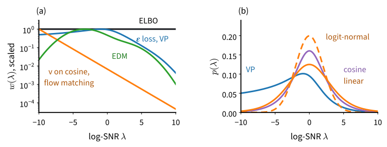
Weightings that fall monotonically in \(\lambda\) are bounds themselves: such an \(\mathcal{L}_w\) is the bound for data augmented with Gaussian noise of a random level (Kingma and Gao 2023), because a weighting that is one below some level \(\mu\) and zero above is the bound Equation 17.5.10 for data noised to log-SNR \(\mu\), and a monotone weighting is a positive mixture of such steps. By this criterion \(\mathbf{v}\)-prediction and flow matching are likelihood training of slightly noisy data; DDPM’s noise loss and EDM’s weighting, which both peak, are not.
17.5.2.3 The Time Distribution as Importance Sampling
Training times enter Equation 17.5.11 only through the product \(w(\lambda) = 2c\, p\, |dt/d\lambda|\). In principle the two are separate: for \(\lambda\) drawn from any density \(p(\lambda)\) that covers the range,
\[ \mathcal{L}_w = \mathbb{E}_{\lambda \sim p}\Big[\frac{w(\lambda)}{2\, p(\lambda)}\, \mathbb{E}\big\|\hat{\boldsymbol\epsilon}_{\boldsymbol\theta}(\mathbf{x}_\lambda, \lambda) - \boldsymbol\epsilon\big\|^2\Big], \]
the importance-sampling identity of Section 41.6.2, so \(p(\lambda)\) changes only the variance of the estimate. Uniform \(t\) on the linear-\(\beta\) VP path spends almost half its draws below \(\lambda = -3\) (panel (b) of Figure 17.5.1), where the bound’s integrand is close to zero, and Nichol and Dhariwal (2021) reweighted them for this reason (2). Since in practice nobody divides by \(p(\lambda)\), a time distribution such as the logit-normal of Esser et al. (2024) is a weighting in disguise.
17.5.3 The Design Space
A diffusion paper fixes a path, a target, a weighting, the training levels, a network and a sampler. Karras et al. (2022) separated these choices and showed that most of them can be made independently.
17.5.3.1 EDM’s Table
EDM, as Karras et al. call their method, describes published methods by these columns:
| method | training: path, levels, weighting | network output | sampler |
|---|---|---|---|
| DDPM | VP, linear \(\beta\), \(t\) uniform, simple loss | noise | ancestral chain, 1,000 steps |
| NCSN | \(\mathbf{x}_0 + \sigma\boldsymbol\epsilon\), geometric ladder of \(\sigma\), weight \(\sigma^2\) | score | annealed Langevin dynamics |
| flow matching | linear, \(t\) uniform | velocity | Euler or an adaptive ODE solver |
| EDM | \(\log \bar\sigma \sim \mathcal{N}(-1.2, 1.2^2)\), weight \(1/c_{\mathrm{out}}^2\) | preconditioned clean image | Heun on the \(\rho = 7\) grid |
NCSN (Song and Ermon 2019) (Section 43.5.3) never scales the data (\(\alpha = 1\)), the variance-exploding view. EDM works in these coordinates on every path, \(\bar{\mathbf{x}} = \mathbf{x}/\alpha\) with noise level \(\bar\sigma = \sigma/\alpha\), as ode_sample does.
EDM’s new column is the parameterization. The network \(F\) shares its weights across noise levels, so it should see inputs and produce outputs of unit variance at every level. For data of standard deviation \(\sigma_{\mathrm{data}}\), the denoiser is
\[ D(\bar{\mathbf{x}}; \bar\sigma) = c_{\mathrm{skip}}\, \bar{\mathbf{x}} + c_{\mathrm{out}}\, F(c_{\mathrm{in}}\, \bar{\mathbf{x}};\, \bar\sigma), \qquad c_{\mathrm{in}} = \frac{1}{\sqrt{\bar\sigma^2 + \sigma_{\mathrm{data}}^2}},\quad c_{\mathrm{skip}} = \frac{\sigma_{\mathrm{data}}^2}{\bar\sigma^2 + \sigma_{\mathrm{data}}^2},\quad c_{\mathrm{out}} = \frac{\bar\sigma\, \sigma_{\mathrm{data}}}{\sqrt{\bar\sigma^2 + \sigma_{\mathrm{data}}^2}}, \tag{17.5.12}\]
and trains it on \(\|D - \mathbf{x}_0\|^2\) with weight \(1/c_{\mathrm{out}}^2\), which gives \(F\) a unit-variance target too (10 derives the coefficients). At low noise the denoiser passes its input through (\(c_{\mathrm{skip}} \to 1\), \(c_{\mathrm{out}} \to 0\)) and \(F\) only corrects it; at high noise the output is \(F\)’s guess scaled to the data (\(c_{\mathrm{skip}} \to 0\), \(c_{\mathrm{out}} \to \sigma_{\mathrm{data}}\)).
EDM wraps a network \(F(\mathbf{x}, t)\) in this preconditioning in the coordinates of a path (\(c_{\mathrm{in}} \bar{\mathbf{x}} = \mathbf{x}/n\) with \(n^2 = \sigma^2 + \alpha^2 \sigma_{\mathrm{data}}^2\), finite even at \(\alpha = 0\)) and predicts the clean image; edm_loss draws the log-normal levels and applies the weight.
class EDM(nn.Module):
    """Karras et al.'s preconditioned denoiser on a path; returns x0-hat."""
    def __init__(self, net, path, sigma_data=0.5):
        super().__init__()
        self.net, self.path, self.sigma_data = net, path, sigma_data

    def forward(self, x, t):
        a = self.path.alpha(t).reshape(-1, 1, 1, 1)
        s = self.path.sigma(t).reshape(-1, 1, 1, 1)
        sd = self.sigma_data
        n = torch.sqrt(s ** 2 + (a * sd) ** 2)
        return a * sd ** 2 / n ** 2 * x + s * sd / n * self.net(x / n, t)

def edm_loss(edm, x0):
    """Log-normal noise levels sigma_bar, loss weight 1 / c_out^2."""
    sigma_bar = torch.exp(-1.2 + 1.2 * torch.randn(len(x0), device=x0.device))
    t = edm.path.time_at(-2 * torch.log(sigma_bar))
    x = edm.path.sample(x0, t, torch.randn_like(x0))
    sd = edm.sigma_data
    weight = (sigma_bar ** 2 + sd ** 2) / (sigma_bar * sd) ** 2
    return (weight.reshape(-1, 1, 1, 1) * (edm(x, t) - x0) ** 2).mean()
class EDM(nnx.Module):
"""Karras et al.'s preconditioned denoiser on a path; returns x0-hat."""
def __init__(self, net, path, sigma_data=0.5):
self.net, self.path, self.sigma_data = net, path, sigma_data
def __call__(self, x, t):
a = self.path.alpha(t).reshape(-1, 1, 1, 1)
s = self.path.sigma(t).reshape(-1, 1, 1, 1)
sd = self.sigma_data
n = jnp.sqrt(s ** 2 + (a * sd) ** 2)
return a * sd ** 2 / n ** 2 * x + s * sd / n * self.net(x / n, t)
def edm_loss(edm, x0, key):
"""Log-normal noise levels sigma_bar, loss weight 1 / c_out^2."""
k_sigma, k_eps = jax.random.split(key)
sigma_bar = jnp.exp(-1.2 + 1.2 * jax.random.normal(k_sigma, (len(x0),)))
t = edm.path.time_at(-2 * jnp.log(sigma_bar))
x = edm.path.sample(x0, t, jax.random.normal(k_eps, x0.shape))
sd = edm.sigma_data
weight = (sigma_bar ** 2 + sd ** 2) / (sigma_bar * sd) ** 2
return (weight.reshape(-1, 1, 1, 1) * (edm(x, t) - x0) ** 2).mean()17.5.3.2 Noise Levels Are Scales
What does a noise level remove from an image? Under an orthonormal two-dimensional Fourier transform, white noise of standard deviation \(\sigma\) has power \(\sigma^2\) at every frequency, while images concentrate their power at low frequencies; a frequency is hidden once the noise power exceeds the image’s. The cell plots the power of the test images, averaged over rings of radius \(r\) cycles per image, against three noise levels.
X, y, X_test, _ = d2l.load_fashion_mnist_pm1()
F = torch.fft.fft2(X_test[:, 0], norm='ortho')    # noise has power sigma^2
k = torch.fft.fftfreq(28, 1 / 28, device=X.device)
ring = torch.sqrt(k[:, None] ** 2 + k ** 2).round().long().flatten()
power = (torch.bincount(ring, (F.abs() ** 2).mean(0).flatten())
         / torch.bincount(ring))                  # the mean over each ring
r, power = torch.arange(1, 15), power[1:15].cpu()
d2l.plot(r, [power] + [torch.full((14,), s ** 2) for s in (0.1, 0.3, 1.0)],
         'cycles per image', 'power', xscale='log', yscale='log',
         legend=['images', 'noise, sigma = 0.1', 'sigma = 0.3', 'sigma = 1'])
for s in (0.1, 0.3, 0.5, 1.0, 2.0):
    hidden = (power < s ** 2).nonzero()
    print(f'sigma = {s}: noise dominates from', f'{r[hidden[0]].item()} cycles'
          if len(hidden) else 'no ring below 15')
sigma = 0.1: noise dominates from no ring below 15
sigma = 0.3: noise dominates from 9 cycles
sigma = 0.5: noise dominates from 6 cycles
sigma = 1.0: noise dominates from 4 cycles
sigma = 2.0: noise dominates from 2 cycles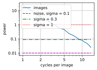
X, y, X_test, _ = d2l.load_fashion_mnist_pm1()
F = jnp.fft.fft2(X_test[..., 0], norm='ortho')    # noise has power sigma^2
k = jnp.fft.fftfreq(28, 1 / 28)
ring = jnp.round(jnp.sqrt(k[:, None] ** 2 + k ** 2)).astype(int).flatten()
power = (jnp.bincount(ring, (jnp.abs(F) ** 2).mean(0).flatten())
         / jnp.bincount(ring))                    # the mean over each ring
r, power = jnp.arange(1, 15), power[1:15]
d2l.plot(r, [power] + [jnp.full((14,), s ** 2) for s in (0.1, 0.3, 1.0)],
         'cycles per image', 'power', xscale='log', yscale='log',
         legend=['images', 'noise, sigma = 0.1', 'sigma = 0.3', 'sigma = 1'])
for s in (0.1, 0.3, 0.5, 1.0, 2.0):
    hidden = jnp.nonzero(power < s ** 2)[0]
    print(f'sigma = {s}: noise dominates from', f'{int(r[hidden[0]])} cycles'
          if len(hidden) else 'no ring below 15')
sigma = 0.1: noise dominates from no ring below 15
sigma = 0.3: noise dominates from 9 cycles
sigma = 0.5: noise dominates from 6 cycles
sigma = 1.0: noise dominates from 4 cycles
sigma = 2.0: noise dominates from 2 cycles
The image power falls by three orders of magnitude from one to fourteen cycles per image. Noise at \(\sigma = 0.1\) stays below it everywhere, \(\sigma = 0.3\) hides the rings from about 9 cycles per image outward, and \(\sigma = 1\) from about 4. Adding noise is thus a low-pass filter whose cutoff falls as \(\sigma\) grows, and sampling runs from coarse to fine: the high-noise steps decide a garment’s silhouette, the last steps its texture (Dieleman 2024).
The same view explains why a schedule depends on the resolution. At \(56 \times 56\) with the same per-pixel noise, averaging each \(2 \times 2\) block recovers the \(28 \times 28\) image while the four noise values average to variance \(\sigma^2/4\): for the coarse structure the signal-to-noise ratio has grown fourfold, and a schedule tuned at one resolution is too easy at a higher one. Hoogeboom et al. (2023) shift \(\lambda_t\) down by the logarithm of the ratio of pixel counts (6, Figure 17.5.2).
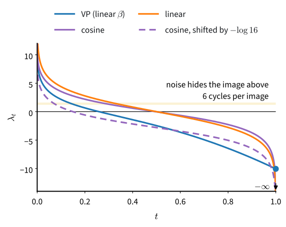
The VP path ends at \(\lambda \approx -10\), so its network never trains on the pure noise the sampler starts from. At high resolution, where block averaging magnifies the leftover signal, this kept Stable Diffusion from generating very bright or very dark images (Lin et al. 2024).
17.5.3.3 A Recipe Ablation
We compare four recipes on Fashion-MNIST with everything else fixed: noise and \(\mathbf{v}\)-prediction on the VP path, the velocity on the linear path (the recipe of Section 17.3), and EDM on the VP path. Each trains an unconditional 64-channel d2l.UNet for 5,000 updates, a third of that section’s budget, and samples the same 1,000 noise images with deterministic and stochastic DDIM (\(\eta = 0\) and \(1\), 50 VP steps) and with 25 Heun steps on its own path, about 50 evaluations each. The Fréchet distance (FD) of Section 17.3 scores the samples against that of two sets of 1,000 test images.
cnn = d2l.fashion_feature_cnn(X, y)
f_test = d2l.fd_features(cnn, X_test[:2000])
floor = d2l.fid_score(f_test[:1000], f_test[1000:])
print(f'FD, real against real: {floor:.2f}')
FD, real against real: 0.88cnn = d2l.fashion_feature_cnn(X, y)
f_test = d2l.fd_features(cnn, X_test[:2000])
floor = d2l.fid_score(f_test[:1000], f_test[1000:])
print(f'FD, real against real: {floor:.2f}')FD, real against real: 0.83A noise predictor cannot be queried at \(\alpha = 0\), so DDIM runs every model on the VP grid, where \(\alpha\) stays positive.
linear = d2l.GaussianPath.linear()
unet = lambda: d2l.UNet(ch=64)
recipes = {  # name: (path, kind of prediction, network, loss)
    'noise, vp': (vp, 'eps', unet, d2l.regression_loss(vp, 'eps')),
    'v, vp': (vp, 'v', unet, d2l.regression_loss(vp, 'v')),
    'velocity, linear': (linear, 'velocity', unet,
                         d2l.regression_loss(linear, 'velocity')),
    'EDM, vp': (vp, 'x0', lambda: EDM(unet(), vp), edm_loss)}
samplers = {  # name: sampler(pred, z, path); DDIM always on the VP time grid
    'DDIM-50, eta 0': lambda pred, z, path: d2l.ddim_sample(pred, z, vp, 50),
    'DDIM-50, eta 1': lambda pred, z, path: d2l.ddim_sample(pred, z, vp, 50,
                                                            1.0),
    'Heun-25': lambda pred, z, path: d2l.heun_sample(pred, z,
                                                     path.sigma_bars(25))}
linear = d2l.GaussianPath.linear()
unet = lambda: d2l.UNet(ch=64, rngs=nnx.Rngs(0))
recipes = { # name: (path, kind of prediction, network, loss)
'noise, vp': (vp, 'eps', unet, d2l.regression_loss(vp, 'eps')),
'v, vp': (vp, 'v', unet, d2l.regression_loss(vp, 'v')),
'velocity, linear': (linear, 'velocity', unet,
d2l.regression_loss(linear, 'velocity')),
'EDM, vp': (vp, 'x0', lambda: EDM(unet(), vp), edm_loss)}
samplers = { # name: sampler(pred, z, path); DDIM always on the VP time grid
'DDIM-50, eta 0': lambda pred, z, path: d2l.ddim_sample(pred, z, vp, 50),
'DDIM-50, eta 1': lambda pred, z, path: d2l.ddim_sample(
pred, z, vp, 50, 1.0, jax.random.key(2)),
'Heun-25': lambda pred, z, path: d2l.heun_sample(pred, z,
path.sigma_bars(25))}The loop trains, samples and scores each model.
batch_fn = lambda: X[torch.randint(0, len(X), (128,), device=X.device)]
samples, fd = {}, {}
for name, (path, kind, make_net, loss_fn) in recipes.items():
    torch.manual_seed(0)
    _, ema_img, _ = d2l.train_regression(make_net().to(device), loss_fn,
                                         batch_fn, 5_000)
    pred = d2l.make_pred(ema_img, path, kind)
    for sampler, run in samplers.items():
        torch.manual_seed(1)                  # the same noise for every run
        z = torch.randn(1000, 1, 28, 28, device=device)
        samples[name, sampler] = run(pred, z, path)
        fd[name, sampler] = d2l.fid_score(
            d2l.fd_features(cnn, samples[name, sampler]), f_test[:1000])
print(f'{"FD":18}' + ''.join(f'{s:>16}' for s in samplers))
for name in recipes:
    print(f'{name:18}' + ''.join(f'{fd[name, s]:16.2f}' for s in samplers))
FD DDIM-50, eta 0 DDIM-50, eta 1 Heun-25
noise, vp 13.38 9.40 10.46
v, vp 8.74 8.36 7.61
velocity, linear 2.97 3.95 2.66
EDM, vp 4.48 6.13 3.87batch_fn = lambda key: X[jax.random.randint(key, (128,), 0, len(X))]
z = jax.random.normal(jax.random.key(1), (1000, 28, 28, 1)) # shared noise
samples, fd = {}, {}
for name, (path, kind, make_net, loss_fn) in recipes.items():
_, ema_img, _ = d2l.train_regression(make_net(), loss_fn, batch_fn, 5_000,
jax.random.key(0))
pred = d2l.make_pred(ema_img, path, kind)
for sampler, run in samplers.items():
samples[name, sampler] = run(pred, z, path)
fd[name, sampler] = d2l.fid_score(
d2l.fd_features(cnn, samples[name, sampler]), f_test[:1000])
print(f'{"FD":18}' + ''.join(f'{s:>16}' for s in samplers))
for name in recipes:
print(f'{name:18}' + ''.join(f'{fd[name, s]:16.2f}' for s in samplers))FD DDIM-50, eta 0 DDIM-50, eta 1 Heun-25
noise, vp 21.58 10.59 17.41
v, vp 7.90 8.95 6.79
velocity, linear 3.95 6.81 3.24
EDM, vp 4.64 7.54 4.08Two sets of real images score just under 1 against each other, and every entry is about three times that or more: 5,000 updates leave all four models far from the data. The recipes separate clearly. The velocity on the linear path scores best with every sampler, with EDM next; \(\mathbf{v}\)-prediction on the VP path lands at two to three times the velocity model’s FD with the deterministic samplers; and the noise predictor’s deterministic samples are the worst entries, with stochastic DDIM better. Apart from the noise predictor, deterministic sampling is about as good as stochastic or better. Below are the noise predictor’s samples (rows: DDIM with \(\eta = 0\), \(\eta = 1\), Heun).
rows = [samples['noise, vp', s][:10] for s in samplers]
d2l.show_gray(torch.cat(rows), 3, 10);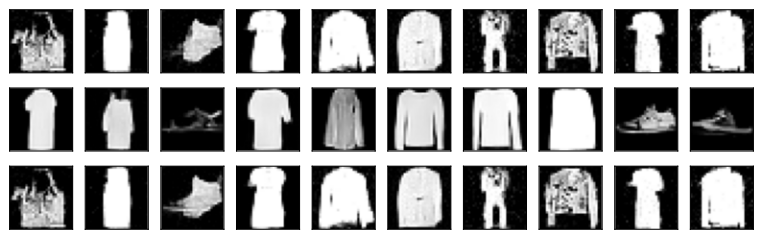
rows = [samples['noise, vp', s][:10] for s in samplers]
d2l.show_gray(jnp.concatenate(rows), 3, 10);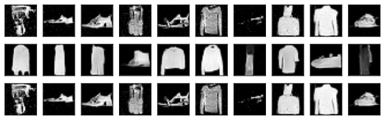
The deterministic samples are blotchy and over-saturated, the stochastic ones smoother garments. At \(t = 1\) the VP path has \(\alpha_1 \approx 0.007\), so \(\hat{\mathbf{x}}_0 = (\mathbf{x} - \sigma\hat{\boldsymbol\epsilon})/\alpha\) magnifies the noise predictor’s error about 150-fold, and the noise loss gives these levels too little weight for a short run to make that error small. The velocity loss weights these levels heavily, and EDM’s network outputs the clean image there without dividing. The \(\mathbf{v}\)-loss, about \(2 \cdot 10^4\) times the noise loss at \(t = 1\), weights them heavily too, yet trails the velocity model, a gap that 4 probes. A stochastic step replaces part of the point with fresh noise and so corrects earlier errors, which a deterministic step carries to the end (Section 17.4).
17.5.3.4 Parameterization at Finite Capacity
For an unlimited network the four targets are one posterior mean in four forms, and choosing among them only chooses a weighting. A finite network finds some harder than others: an image lies near a set of much lower dimension than its pixel count, while the noise fills every dimension, so the clean image is the simpler target at every level. Li and He (2026) find that transformers on large patches fail at predicting the noise or the velocity and work at predicting the clean image.
17.5.4 Summary
Diffusion training is maximum likelihood up to a weighting. The chain’s bound is a sum of noise regressions weighted by the drop in log-SNR per step, and on the mixture the trained network’s bound and its probability-flow likelihood both come within about \(0.01\) nats of the true 2.5 nats. DDPM’s simple loss, \(\mathbf{v}\)-prediction, flow matching and EDM are the same integral with other weightings; the monotone ones are bounds for noise-augmented data. The parameterization decides what a finite network must compute, and the schedule matters through its endpoints and the resolution. Most of an image’s pixels carry detail a viewer hardly sees: why diffuse the pixels at all, rather than a smaller representation?
17.5.5 Exercises
- [code] The prior term. The reverse chain starts from \(\mathcal{N}(\mathbf{0}, \mathbf{I})\), and \(L_T\) measures how far the end of the forward chain is from it.
- Approximating \(\log(1 - \beta_k)\) by \(-\beta_k\) gives \(\alpha_T^2 \approx \exp(-\sum_k \beta_k)\). Evaluate the approximation for the VP path’s chain at \(T = 1000\) and compare it with the exact value. Which term of the expansion of \(\log(1 - \beta_k)\) accounts for the difference?
- Use Equation 16.1.8 to write \(L_T\) as a function of \(\alpha_T^2\), \(d\) and \(\|\mathbf{x}_0\|^2\), and show that it is approximately \(\tfrac12 \alpha_T^2 \|\mathbf{x}_0\|^2\) for small \(\alpha_T^2\). Compute \(\mathbb{E}\|\mathbf{x}_0\|^2\) for the mixture from its parameters and evaluate \(L_T\) for
vpand for a VP path with \(\beta\) from \(0.1\) to \(5\). - For the second path, draw 20,000 samples with
d2l.ancestral_sampleand the exact predictor, once starting from \(\mathcal{N}(\mathbf{0}, \mathbf{I})\) and once from the exact \(q(\mathbf{x}_T)\), which you obtain by noising draws of the mixture. Compare the outputs ofmix.summary. Which statistic does the prior term affect? Compute the mean of \(q(\mathbf{x}_T)\) and use it to explain the direction of the change. (The extended exercise “Prior mismatch, ODE versus SDE” of Section 43.4 compares how the reverse SDE and the probability-flow ODE carry such a mismatch to the data.)
- [code] The weights of the bound. ● Let \(w_k\) be the weight in Equation 17.5.9.
- Compute \(w_k\) for \(\nu_k = \beta_k\) and for \(\nu_k = \tilde\beta_k\) at every step \(k = 2, \ldots, 1000\) of the VP chain and plot both on a logarithmic axis. What fraction of \(\sum_k w_k\) lies on the steps \(k \le 20\) for each choice? What fraction does the simple loss put there?
- Evaluate the chain’s bound Equation 17.5.4 on the mixture with the exact noise predictor, \(\nu_k = \tilde\beta_k\), and the reconstruction term of the text at the noise level of step 1. Compare it with the true negative log-likelihood and with the continuous bound of the text. Show that over a step where the clean point is uncertain by about the step’s own noise, the true reverse step has a variance larger than \(\tilde\beta_k\), and estimate the divergence that each of the first steps contributes. Repeat with steps uniform in \(\lambda\) instead of \(t\).
- A minibatch estimate of the chain’s bound draws \(k\) uniformly. Nichol and Dhariwal (2021) (Section 3.3) instead draw \(k\) with probability \(p_k\) proportional to the root mean square of the per-sample value of \(L_{k-1}\) and divide the drawn term by \(p_k\). Why does this reduce the variance of the estimate? Which steps would such a sampler draw most often on the mixture?
- [code] Target and weighting. ● Ho et al. (2020) (Table 2) compare predicting \(\tilde{\boldsymbol\mu}_k\) with predicting \(\boldsymbol\epsilon\), each trained on the bound or on an unweighted squared error.
- Let the network output \(\boldsymbol\mu_{\boldsymbol\theta}\) directly and train it on Equation 17.5.6 with \(\nu_k = \beta_k\). Solve Equation 17.5.8 for the implied noise prediction, and show that in terms of it the objective is the regression Equation 17.5.9 with the weights of the bound. What must a network that outputs \(\boldsymbol\mu_{\boldsymbol\theta}\) represent accurately, given that \(\tilde{\boldsymbol\mu}_k\) is nearly \(\mathbf{x}_k\)?
- With
TimeMLPand the recipe of this section on the chain with \(T = 1000\), train three models: noise prediction with the weights of the bound, mean prediction on the bound, and mean prediction on the unweighted error. Compare each with the model trained on the simple loss by the bound and the flow likelihood of the text, and by the summary statistics of DDIM samples with 50 steps. Which findings of Ho et al. (2020) does the comparison reproduce?
- The implied weighting. Use Equation 17.5.11.
- Show that the velocity loss on the linear path with \(t\) uniform has \(w(\lambda) \propto e^{-\lambda/2}\), and that the \(\mathbf{v}\)-loss on the cosine path \(\alpha_t = \cos\frac{\pi t}{2}\), \(\sigma_t = \sin\frac{\pi t}{2}\) has the same weighting.
- Show that the noise loss on the cosine path with \(t\) uniform has \(w(\lambda) \propto \cosh^{-1}(\lambda/2)\), and compute \(w\) for the noise loss and the \(\mathbf{v}\)-loss on the linear-\(\beta\) VP path of the ablation.
- Which of these weightings are monotone in \(\lambda\)? Which noise levels does the noise loss on the VP path downweight relative to the \(\mathbf{v}\)-loss on the same path, and by what factor at its last step?
- (Code.) By the first part, the \(\mathbf{v}\)-loss on the cosine path weights the levels as the velocity loss does. Train it with the recipe of the ablation and score it with the three samplers. Does matching the weighting close the gap between \(\mathbf{v}\)-prediction on the VP path and the velocity model? What else differs between the two recipes?
- [code] Likelihoods in many dimensions. ● In \(d\) dimensions the exact divergence in
pf_nlltakes \(d\) forward-mode derivatives per evaluation. Replace it by the estimate \(\mathbf{r}^\top (\partial \mathbf{u}/\partial \mathbf{x})\, \mathbf{r}\) of Equation 43.2.11 with one Rademacher vector \(\mathbf{r}\) per step, which takes one derivative (Grathwohl et al. 2019).- Show that the resulting estimate of \(\log p\) is unbiased. The variance of one probe is derived in Exercise 6a; measure the standard deviation of the estimate per point on the mixture, and compare it with the gap of a few thousandths of a nat between the trained network and the exact field. How many probes per step, or how many points, does resolving that gap take?
- Apply the estimate to the velocity model of the ablation on 100 test images, after adding uniform noise of the width of one gray level, \(2/255\), to each pixel. Report the result in bits per dimension, \(\big(-\log p(\mathbf{x})/d + \log 127.5\big)/\log 2\), which counts the bits per pixel of the 8-bit image. Compare it with the 8 bits of the raw encoding. What would 15,000 updates change?
- Resolution and the schedule. Write \(\mathrm{SNR}_t = \alpha_t^2/\sigma_t^2\) for data with unit variance per pixel.
- Show that multiplying the data by a constant \(\kappa\) multiplies the ratio of signal to noise variance in \(\mathbf{x}_t\) by \(\kappa^2\) at every \(t\).
- Upsample each image to \(28 r \times 28 r\) pixels by repeating every pixel in an \(r \times r\) block, and noise the large image with the same schedule. Show that averaging the noisy image over the blocks gives the original image at the ratio \(r^2\, \mathrm{SNR}_t\).
- For \(r = 32\), an \(896 \times 896\) image, compute \(r^2\, \mathrm{SNR}_1\) for
vp, and find the time of the \(28 \times 28\) path with the same ratio. What does the result imply for an \(896 \times 896\) model trained with this schedule, whose sampler starts from pure noise? - Which shift of \(\lambda_t\) lets the averaged large image pass through the same ratios as the \(28 \times 28\) model? Compare it with the shift of Hoogeboom et al. (2023) .
- [code] Paired likelihood comparisons. Differences of hundredths of a nat between two models can only be resolved by pairing.
- For a fixed model \(p_{\boldsymbol\theta}\) and test points \(\mathbf{x}_i\), let \(d_i = \log p(\mathbf{x}_i) - \log p_{\boldsymbol\theta}(\mathbf{x}_i)\). Show that the mean of the \(d_i\) is an unbiased estimate of \(D_{\textrm{KL}}(p \,\|\, p_{\boldsymbol\theta})\). Why can it be negative?
- Train a velocity model on the linear path with the recipe of this section. Compute the flow likelihood of both models on the same 4,000 test points, and report each model’s mean negative log-likelihood with its standard error, then the mean of the per-point differences with its standard error. Which comparison resolves the two models? (Section 41.4.2.6 discusses the general case.)
- Do the same for the bound. Its log-SNR form is the same on every path, so for the velocity model draw \(\lambda\), find the time of the linear path with
time_at, and turn the velocity prediction into a noise prediction withx0_eps. Does the ordering of the two models agree with that of the flow likelihood?
- The forward posterior. Derive Equation 17.5.5.
- Write \(q(\mathbf{x}_{k-1} \mid \mathbf{x}_k, \mathbf{x}_0) \propto q(\mathbf{x}_k \mid \mathbf{x}_{k-1})\, q(\mathbf{x}_{k-1} \mid \mathbf{x}_0)\) as a product of two Gaussians in \(\mathbf{x}_{k-1}\), add their precisions, and combine their means in proportion to precision.
- Show that \(\tilde\beta_k \le \beta_k\), with equality only if \(\sigma_{k-1}^2 = 1\). Where in the chain is \(\tilde\beta_k\) much smaller than \(\beta_k\)?
- For \(T = 2\) and \(\beta_1 = \beta_2 = 1/2\), write out \(\tilde{\boldsymbol\mu}_2\) and \(\tilde\beta_2\), and the three terms of Equation 17.5.4 for a network that predicts the noise exactly, for one-dimensional data \(\mathcal{N}(0, s^2)\).
- [code] Clipping the predicted image. The cosine path reaches \(\alpha_1 = 0\).
- Train a noise predictor on
d2l.GaussianPath.cosine()with the recipe of the ablation and sample it withddim_sampleon the same path. What happens at the first step, and why? - Start the sampler instead at \(t = 0.99\) from pure noise, with
t_start. Compare the samples and their FD with those of the noise predictor of the ablation. - Wrap the predictor so that it clips \(\hat{\mathbf{x}}_0\) to \([-1, 1]\) and recomputes \(\hat{\boldsymbol\epsilon}\) from it, and sample again. Which part of the failure does clipping repair, and which does it not? Why does a \(\mathbf{v}\)-predictor on the same path need no clipping?
- Train a noise predictor on
- EDM’s preconditioning. ● Let \(\mathbf{x}_0\) have zero mean and per-coordinate variance \(\sigma_{\mathrm{data}}^2\), independent of the noise.
- Choose \(c_{\mathrm{in}}\) so that the input \(c_{\mathrm{in}}(\mathbf{x}_0 + \bar\sigma\boldsymbol\epsilon)\) of \(F\) has unit variance. Writing the training target of \(F\) as \((\mathbf{x}_0 - c_{\mathrm{skip}}\, \bar{\mathbf{x}})/c_{\mathrm{out}}\), choose \(c_{\mathrm{skip}}\) to minimize its variance, and then \(c_{\mathrm{out}}\) to make that variance one. Check the result against Equation 17.5.12.
- Show that the loss \(\|D - \mathbf{x}_0\|^2 / c_{\mathrm{out}}^2\) is \(\|F - \textrm{target}\|^2\), and that, written as a noise loss, it is the noise error times \((e^{-\lambda} + \sigma_{\mathrm{data}}^2)/\sigma_{\mathrm{data}}^2\).
- With \(\log \bar\sigma \sim \mathcal{N}(-1.2, 1.2^2)\), show that EDM’s weighting is \(w(\lambda) \propto \mathcal{N}(\lambda; 2.4, 2.4^2)\, (e^{-\lambda} + \sigma_{\mathrm{data}}^2)\). Where is its peak? Kingma and Gao (2023) make it monotone by holding it at its peak value for all \(\lambda\) below the peak. By the theorem of the text, what does the change make of EDM’s objective?