%matplotlib inline
from d2l import torch as d2l
import torch
import numpy as np27.1 Random Variables
In Section 1.6 we considered discrete random variables, whose probabilities are obtained by summing probability masses. Pixel intensities, network weights, and Gaussian noise are usually modeled as continuous random variables, for which individual outcomes have probability zero. A probability density assigns probability to intervals through integration. This section develops densities and cumulative distribution functions, then introduces the mean, variance, and standard deviation. Joint, marginal, and conditional distributions extend the same definitions to several variables, together with covariance and correlation. The relation in Equation 27.1.1 connects the probability of a small interval to its width and local density.
%matplotlib inline
from d2l import tensorflow as d2l
import tensorflow as tf
import numpy as np%matplotlib inline
from d2l import jax as d2l
from jax import numpy as jnp
import numpy as np%matplotlib inline
from d2l import mxnet as d2l
from mxnet import np, npx
npx.set_np()27.1.1 From Discrete to Continuous Probability
For a continuous random variable, probabilities are obtained by integrating rather than summing. We develop the theory in three steps: first the density that replaces the mass function, the cumulative function that turns it back into a genuine probability, and the derivative relationship between them, which is the fundamental theorem of calculus restated for probabilities.
27.1.1.1 From Bin Probabilities to a Density
Throw a dart at a board and ask for the probability it lands exactly \(2\,\textrm{cm}\) from the center. Measure to one digit, with bins for \(0,1,2,\ldots\,\textrm{cm}\): of \(100\) throws, perhaps \(20\) land in the “\(2\,\textrm{cm}\)” bin, suggesting \(20\%\). But that bin holds everything between \(1.5\) and \(2.5\,\textrm{cm}\), not what we asked. Measure finer, to bins of \(0.1\,\textrm{cm}\): now perhaps \(3\) throws land in \([1.95,2.05]\), suggesting \(3\%\). We have only pushed the problem one digit down.
The relevant object is the probability of a short interval, not the behavior of successive decimal digits. For \(\epsilon>0\), consider \(P(x\leq X<x+\epsilon)\). If the local probability-to-width ratio has a limit, define
\[ p(x)=\lim_{\epsilon\downarrow0} \frac{P(x\leq X<x+\epsilon)}{\epsilon}. \]
At points where \(p\) is continuous, this definition gives
\[P(x\leq X<x+\epsilon)=\epsilon p(x)+o(\epsilon). \tag{27.1.1}\]
When interval probabilities have the representation \(P(X\in A)=\int_A p(x)\,dx\), the law is absolutely continuous and \(p\) is its probability density function (p.d.f.). Not every probability law has a density; discrete laws have atoms, and mixed laws contain both atomic and density parts.
If \(X\) has a density, every singleton has zero probability. Thus, for any fixed \(x\),
\[P(X = x) = 0.\]
This resolves the dartboard example: the probability of landing exactly \(2\,\textrm{cm}\) out is zero, even though the dart certainly lands somewhere. The size notion at work here deserves a name. A set has measure zero when, for every \(\varepsilon>0\), it can be covered by a countable collection of intervals of total length at most \(\varepsilon\): a single point fits inside one interval of length \(\varepsilon\), and a countable set \(\{x_1,x_2,\ldots\}\) fits inside intervals of lengths \(\varepsilon/2,\varepsilon/4,\ldots\), which sum to \(\varepsilon\). For a variable with a density, every measure-zero set carries zero probability: covering the set by intervals of total length \(\delta\) caps its probability at the integral of \(p\) over those intervals, which shrinks to zero with \(\delta\) (immediately when \(p\) is bounded, and with a little more care in general). A point carrying positive mass is called an atom. A purely absolutely continuous variable has no atoms, whereas a mixed law may have atoms and a density on the remainder of its support.
27.1.1.2 Densities and Their Two Defining Properties
What must \(p(x)\) satisfy to be a density? Two things, both from Equation 27.1.1. First, probabilities are never negative, so \(p(x)\ge 0\). Second, slice \(\mathbb{R}\) into width-\(\epsilon\) pieces \((\epsilon i, \epsilon(i{+}1)]\); by Equation 27.1.1 each contributes about \(\epsilon\, p(\epsilon i)\) to the total probability, and summing,
\[ P(X\in\mathbb{R}) \approx \sum_i \epsilon \cdot p(\epsilon\cdot i) \;\xrightarrow[\epsilon\to0]{}\; \int_{-\infty}^{\infty} p(x)\,dx . \]
The middle expression is exactly the Riemann sum of Section 25.4. Since \(X\) must take some value, \(P(X\in\mathbb{R})=1\), and we recover the normalization \(\int_{-\infty}^{\infty} p(x)\,dx = 1\) of Equation 25.4.11. The same slicing argument over a finite range gives the rule we actually use: probability is area under the density,
\[P(X\in(a, b]) = \int_{a}^{b} p(x)\,dx. \tag{27.1.2}\]
These two properties, non-negativity and total area \(1\), describe exactly the space of densities. Figure 27.1.1 shows the picture: the total shaded region has area \(1\), and the probability of an interval is the area above it.
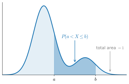
We can confirm Equation 27.1.2 numerically. Take the two-bump density \(p(x)=0.2\,\mathcal N(x;3,1)+0.8\,\mathcal N(x;-1,1)\) and recover the probability of an interval by a Riemann sum, the discrete approximation of the integral.
import numpy as onp
# Recover P(-2 < X <= 3) from the density by a Riemann sum (numerical integral)
epsilon = 0.01
x = onp.arange(-8, 8, epsilon)
p = 0.2*onp.exp(-(x - 3)**2 / 2)/onp.sqrt(2 * onp.pi) + \
    0.8*onp.exp(-(x + 1)**2 / 2)/onp.sqrt(2 * onp.pi)
print(f'total mass     : {float(onp.sum(epsilon * p)):.4f}')
mask = (x > -2) & (x <= 3)
print(f'P(-2 < X <= 3) : {float(onp.sum(epsilon * p[mask])):.4f}')
total mass : 1.0000
P(-2 < X <= 3) : 0.7725The total mass is \(1.0000\), as Equation 25.4.11 requires (the grid spans \([-8,8]\), wide enough that the truncated Gaussian tails hold mass under \(10^{-7}\)), and the interval integral returns a genuine probability in \([0,1]\). The estimate \(0.7725\) is within \(6\times10^{-4}\) of the exact value \(0.7731\), the small bias of a left-endpoint Riemann sum at \(\epsilon=0.01\). A catalogue of named densities (Gaussian, exponential, and the rest) follows in Section 27.2; here we stay abstract.
27.1.1.3 The Cumulative Distribution Function
A density has one awkward feature: its values are not probabilities. A density can exceed \(10\), as long as it does so only over an interval shorter than \(1/10\). The remedy is the cumulative distribution function (c.d.f.), which by Equation 27.1.2 accumulates the density up to \(x\) and so is a probability:
\[ F(x) = \int_{-\infty}^{x} p(t)\,dt = P(X \le x). \tag{27.1.3}\]
Read off its properties directly: \(F(x)\to 0\) as \(x\to-\infty\) and \(F(x)\to 1\) as \(x\to+\infty\) (the total mass is \(1\)); \(F\) is non-decreasing, since the integrand \(p\ge 0\) only ever adds area; and since \(X\) has a density, \(F\) is an integral of it and hence continuous. The c.d.f. is also what lets discrete and continuous variables share one framework. For a discrete \(X\) taking \(0\) and \(1\) with probability \(\tfrac12\) each,
\[ F(x) = \begin{cases} 0 & x < 0, \\ \tfrac12 & 0 \le x < 1, \\ 1 & x \ge 1, \end{cases} \]
a staircase that jumps by the mass at each atom. The same \(F\) thus describes continuous variables, discrete ones, and mixtures (flip a coin: heads, report a die roll; tails, a dart distance).
The density and the c.d.f. carry the same information, and the bridge between them is the fundamental theorem of calculus. Differentiating Equation 27.1.3 recovers the density.
Proposition (density is the derivative of the c.d.f.). If \(X\) has a continuous density \(p\), then \(F\) is differentiable and
\[ F'(x) = p(x). \tag{27.1.4}\]
Proof. By definition Equation 27.1.3, \(F(x)=\int_{-\infty}^x p(t)\,dt\) is the area-so-far function of the integrand \(p\). The fundamental theorem of calculus Equation 25.4.3 says precisely that such an area function is differentiable with derivative equal to the integrand, \(F'(x)=p(x)\), at every point where \(p\) is continuous. \(\blacksquare\)
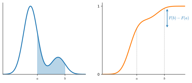
So \(p=F'\) and \(F=\int p\) are two views of one object: the density is the instantaneous rate at which probability accumulates, and the c.d.f. is the accumulated area. Figure 27.1.2 puts them side by side (the shaded area \(\int_a^b p\) on the left equals the vertical rise \(F(b)-F(a)\) on the right), making Equation 27.1.3 and Equation 27.1.4 a single picture.
The inverse \(F^{-1}\), which maps a probability level \(q\in(0,1)\) back to the value \(x\) with \(F(x)=q\), is called the quantile function; its values at \(q=0.25,0.5,0.75\) are the quartiles, the middle one the median. The quantile function is also a sampler, by an argument short enough to give in full. The argument needs one ingredient: a variable \(U\) uniform on \([0,1]\), the variable whose density is constant at \(1\) there, so that \(U\) assigns every subinterval of \([0,1]\) probability equal to its length (Section 27.2 names this law \(U(0,1)\)).
Proposition (inverse-transform sampling). Let \(F\) be a continuous, strictly increasing c.d.f. and let \(U\) be uniform on \([0,1]\). Then \(X=F^{-1}(U)\) has c.d.f. exactly \(F\).
Proof. Because \(F\) is increasing, the events \(F^{-1}(U)\le x\) and \(U\le F(x)\) are the same event, and the uniform assigns the latter probability \(F(x)\), the length of the subinterval \([0,F(x)]\):
\[ P\bigl(F^{-1}(U)\le x\bigr) = P\bigl(U\le F(x)\bigr) = F(x). \quad\blacksquare \]
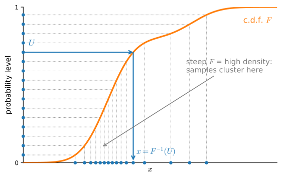
Figure 27.1.3 illustrates the construction. Place the uniform level \(U\) on the vertical axis of the c.d.f. and map it through the curve to the horizontal axis. Where the density is high, the c.d.f. is steep, so a uniform range of vertical levels maps to a narrow range of horizontal values. Thus the transformed samples are concentrated where the density is large. This proposition gives a general procedure for turning uniform noise into samples from a one-dimensional distribution: generate \(U\), then evaluate \(F^{-1}(U)\). We put it to work when we meet the named distributions in Section 27.2, where inverting the exponential’s c.d.f. gives that distribution’s standard sampler in closed form.
Sampling is also how expectations are computed at scale: given independent draws \(x_1,\ldots,x_n\) of \(X\), the Monte Carlo estimate \(\tfrac1n\sum_{i=1}^n g(x_i)\) approximates \(E[g(X)]\), and its variance is \(\textrm{Var}(g(X))/n\) (Exercise 6 carries out the computation), shrinking with every additional sample. The guarantee that the estimate converges to the expectation, the law of large numbers, is stated and proved in Section 27.5.
27.1.2 Summarizing a Distribution
A full distribution is often more than we can interpret at a glance. Summary statistics reduce it to a few numbers: the mean locates its center, while the variance and standard deviation measure its spread. Each is an expectation, that is, a density-weighted average as in Equation 25.4.12. We derive their basic algebra once and use it throughout the book.
27.1.2.1 The Mean
The mean (or expectation) is the average value, weighting each outcome by its probability. For a discrete \(X\) taking \(x_i\) with probability \(p_i\),
\[\mu_X = E[X] = \sum_i x_i p_i, \tag{27.1.5}\]
and in the continuum the sum becomes the density-weighted integral Equation 25.4.12, \(\mu_X=\int x\,p(x)\,dx\), by the same slice-and-refine argument that produced the normalization Equation 25.4.11. The same weighting averages any function of \(X\): \(E[g(X)]=\sum_i g(x_i)\,p_i\) in the discrete case, while the continuous form \(\int g(x)\,p(x)\,dx\) restates the second half of Equation 25.4.12. We apply the rule so routinely and so silently that it has earned a name: the law of the unconscious statistician. It applies below whenever we average \(X^2\) or a squared deviation; only the name and the discrete form are new here. The mean describes the center of a distribution, although it need not be a typical value.
A running example recurs through the whole section. Let \(X\) take \(a-2\) with probability \(p\), \(a+2\) with probability \(p\), and \(a\) with probability \(1-2p\). Then
\[ \mu_X = (a-2)p + a(1-2p) + (a+2)p = a, \]
the center of symmetry, exactly as intuition demands.
The most frequently used algebraic property of the mean is linearity: constants may be taken outside an expectation, and the expectation of a sum is the sum of the expectations. Both statements follow directly from the definition.
Proposition (linearity of expectation). For random variables \(X,Y\) and constants \(a,b\),
\[ E[aX+b]=a\,E[X]+b, \qquad E[X+Y]=E[X]+E[Y]. \tag{27.1.6}\]
Proof. Both are linearity of the sum (or integral) defining the expectation. For the scaling-and-shift, \(E[aX+b]=\sum_i(ax_i+b)p_i = a\sum_i x_i p_i + b\sum_i p_i = a\,E[X]+b\), using \(\sum_i p_i=1\). For the sum, write the expectation over the joint distribution of \((X,Y)\), with \(p_{ij}\) the probability of the pair \((x_i,y_j)\) (the discrete joint of Section 1.6; its continuous counterpart, the joint density, arrives later in this section), and split the inner sum: \(E[X+Y]=\sum_{i,j} (x_i+y_j)p_{ij} = \sum_{i,j} x_i p_{ij} + \sum_{i,j} y_j p_{ij} = E[X]+E[Y]\), the last step recognizing the marginals \(\sum_j p_{ij}=P(X=x_i)\). The continuous case replaces every sum by an integral verbatim. \(\blacksquare\)
The second identity needs no independence assumption: expectations of sums always add, however entangled \(X\) and \(Y\) are. Expected-loss calculations throughout the book rest on this.
The mean alone is not enough. A profit of \(\$10\pm\$1\) per sale and one of \(\$10\pm\$15\) share a mean but carry wildly different risk. We need a measure of spread.
27.1.2.2 Variance and Standard Deviation
The variance measures how far \(X\) strays from its mean. The deviation \(X-\mu_X\) is positive or negative, so we square it before averaging:
\[\sigma_X^2 = \textrm{Var}(X) = E\bigl[(X-\mu_X)^2\bigr]. \tag{27.1.7}\]
Expanding the square gives a formula that is almost always easier to compute with, and it deserves a proof since we use it constantly.
Proposition (computational form of the variance).
\[ \textrm{Var}(X) = E[X^2] - E[X]^2 = E[X^2]-\mu_X^2. \tag{27.1.8}\]
Proof. Expand the square inside Equation 27.1.7 and apply linearity Equation 27.1.6, treating \(\mu_X\) as the constant it is:
\[ E\bigl[(X-\mu_X)^2\bigr] = E\bigl[X^2 - 2\mu_X X + \mu_X^2\bigr] = E[X^2] - 2\mu_X\,E[X] + \mu_X^2 = E[X^2] - \mu_X^2, \]
since \(E[X]=\mu_X\), so \(-2\mu_X E[X]+\mu_X^2 = -2\mu_X^2+\mu_X^2=-\mu_X^2\). \(\blacksquare\)
On the running example \(\mu_X=a\), and the computational form does the rest: \(E[X^2]=(a-2)^2p+a^2(1-2p)+(a+2)^2p = a^2+8p\), so
\[ \textrm{Var}(X) = E[X^2]-\mu_X^2 = (a^2+8p)-a^2 = 8p. \]
This is sensible: at the largest allowed \(p=\tfrac12\) the variable is a coin flip between \(a\pm2\), each \(2\) away from the mean, giving variance \(8\cdot\tfrac12=4=2^2\); at \(p=0\) it is constant at \(a\) with no variance at all.
How does variance behave under the affine maps we constantly apply (rescaling units, centering data)? The shift drops out and the scale comes out squared.
Proposition (variance under affine maps). For constants \(a,b\),
\[ \textrm{Var}(aX+b) = a^2\,\textrm{Var}(X). \tag{27.1.9}\]
Proof. By linearity Equation 27.1.6 the mean maps as \(\mu_{aX+b}=a\mu_X+b\), so the deviation is \((aX+b)-\mu_{aX+b}=a(X-\mu_X)\); the shift \(b\) cancels. Squaring and taking the expectation,
\[ \textrm{Var}(aX+b) = E\bigl[a^2(X-\mu_X)^2\bigr] = a^2\,E\bigl[(X-\mu_X)^2\bigr] = a^2\,\textrm{Var}(X). \qquad\blacksquare \]
Two further facts round out the list: \(\textrm{Var}(X)\ge 0\), with equality iff \(X\) is constant (a square has non-negative mean, zero only when \(X-\mu_X\equiv0\)); and for independent \(X,Y\), \(\textrm{Var}(X+Y)=\textrm{Var}(X)+\textrm{Var}(Y)\) (we prove the general version, with a covariance correction, in Section 27.1.3.4).
The variance has a units problem. If \(X\) is in stars, \(X-\mu_X\) is in stars but \((X-\mu_X)^2\) is in squared stars, so \(\textrm{Var}(X)\) is not comparable to the data. Taking the square root restores the original units and defines the standard deviation
\[ \sigma_X = \sqrt{\textrm{Var}(X)}. \tag{27.1.10}\]
Its properties echo the variance through the square root: \(\sigma_X\ge0\); \(\sigma_{aX+b}=|a|\sigma_X\) (the absolute value because \(\sqrt{a^2}=|a|\)); and for independent \(X,Y\), \(\sigma_{X+Y}=\sqrt{\sigma_X^2+\sigma_Y^2}\). On the running example \(\sigma_X=2\sqrt{2p}\), back in units of stars.
27.1.2.3 Markov’s and Chebyshev’s Inequalities
The standard deviation \(\sigma_X\) sets the scale of typical fluctuations. Two inequalities make this statement precise for any distribution. The first, Markov’s inequality, turns the mean into a tail bound: a non-negative variable cannot assign much probability to values far above its mean.
Proposition (Markov’s inequality). If \(X\ge 0\) and \(a>0\), then
\[ P(X \ge a) \le \frac{E[X]}{a}. \tag{27.1.11}\]
Proof. Let \(\mathbf{1}_{X\ge a}\) be the indicator variable that is \(1\) when \(X\ge a\) and \(0\) otherwise. Then \(X \ge a\,\mathbf{1}_{X\ge a}\) pointwise: on the event \(\{X\ge a\}\) the right-hand side is \(a\le X\), and elsewhere it is \(0\le X\). Taking expectations of both sides and using \(E[\mathbf{1}_{X\ge a}]=P(X\ge a)\) gives \(E[X]\ge a\,P(X\ge a)\). \(\blacksquare\)
So at most a tenth of any non-negative population exceeds ten times its average: true of incomes, file sizes, and gradient norms alike, with no distributional assumption whatsoever. On its own the bound is crude, because it knows only the mean. But feed it the squared deviation \((X-\mu_X)^2\), whose mean is by definition the variance, and it sharpens into the statement we are after, an inequality due to Bienaymé and to Chebyshev (Chebyshev 1867).
Proposition (Chebyshev’s inequality). For any \(X\) with finite variance and any \(\alpha>0\),
\[P\bigl(|X - \mu_X| \ge \alpha\sigma_X\bigr) \le \frac{1}{\alpha^2}. \tag{27.1.12}\]
Proof. The variable \(Z=(X-\mu_X)^2\) is non-negative with \(E[Z]=\textrm{Var}(X)=\sigma_X^2\) by Equation 27.1.7, and the event \(\{|X-\mu_X|\ge\alpha\sigma_X\}\) is exactly the event \(\{Z\ge\alpha^2\sigma_X^2\}\). Markov’s inequality Equation 27.1.11 with \(a=\alpha^2\sigma_X^2\) gives \(P(|X-\mu_X|\ge\alpha\sigma_X) \le \sigma_X^2/(\alpha^2\sigma_X^2) = 1/\alpha^2\). \(\blacksquare\)
Corollary (\(\varepsilon\)-form). For any \(X\) with finite variance and any \(\varepsilon>0\),
\[ P\bigl(|X-\mu_X| \ge \varepsilon\bigr) \le \frac{\textrm{Var}(X)}{\varepsilon^2}. \]
Setting \(\varepsilon=\alpha\sigma_X\) recovers Equation 27.1.12 when \(\sigma_X>0\); applying Markov’s inequality to \((X-\mu_X)^2\) with \(a=\varepsilon^2\) proves the corollary directly and covers the edge case \(\sigma_X=0\), where \(X\) equals its mean with probability one and the left-hand side is \(0\). This is the form Section 24.1 invoked for the concentration of random angles.
In words at \(\alpha=10\): for any distribution at most \(1\%\) of the mass lies ten or more standard deviations from the mean; at least \(99\%\) lies strictly within. The standard deviation is thus a universal yardstick for “how far is far.”
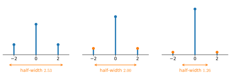
The bound is sharp: our running example shows why no smaller constant can hold in general. With \(\mu_X=a\) and \(\sigma_X=2\sqrt{2p}\), Chebyshev’s inequality at \(\alpha=2\) gives \(P\bigl(|X-a|\ge 4\sqrt{2p}\bigr)\le\tfrac14\). The two outlying atoms \(a\pm2\) are at distance exactly \(2\), and as \(p\) decreases the threshold \(4\sqrt{2p}\) shrinks with it. Figure 27.1.4 shows the three regimes. For \(p>\tfrac18\) the threshold exceeds \(2\), no atom lies that far out, and the left-hand side is \(0\): the bound holds with room to spare. At \(p=\tfrac18\) the threshold equals \(2\) exactly (then \(\sigma_X=1\), so \(a\pm2\) are precisely two standard deviations from the mean): both outlying atoms count toward the event, the probability is \(p+p=\tfrac14\), and the bound is attained with equality, so no constant smaller than \(1/\alpha^2\) could work for every distribution. For \(p<\tfrac18\) the threshold drops below \(2\), both atoms lie beyond it, and their combined mass \(2p<\tfrac14\) keeps the inequality satisfied.
27.1.2.4 Means and Variances in the Continuum
The preceding definitions extend to continuous variables by the same limiting argument: slice \(\mathbb{R}\) into width-\(\epsilon\) pieces, apply the discrete definition, and let \(\epsilon\to0\) to turn the sum into an integral. The mean is the density-weighted average Equation 25.4.12, and the variance follows from its computational form Equation 27.1.8:
\[ \mu_X = \int_{-\infty}^\infty x\,p_X(x)\,dx, \qquad \sigma^2_X = \int_{-\infty}^\infty x^2 p_X(x)\,dx - \mu_X^2 . \tag{27.1.13}\]
Every property proved above (linearity, the affine rule, Markov and Chebyshev) carries over unchanged, since each rested only on linearity and positivity of the averaging operation. For the uniform density \(U(0,1)\) met at inverse-transform sampling (\(p(x)=1\) on \([0,1]\), zero elsewhere), \(\mu_X=\int_0^1 x\,dx=\tfrac12\) and \(\sigma_X^2=\int_0^1 x^2\,dx-\tfrac14=\tfrac13-\tfrac14=\tfrac1{12}\), both elementary integrals.
A cautionary example: the Cauchy distribution \(p(x)=\frac{1}{\pi(1+x^2)}\) is a perfectly good density (a table of integrals confirms it integrates to \(1\)), yet it has neither a finite variance nor a well-defined mean. The variance integral \(\int x^2 p(x)\,dx\) diverges because \(\frac{x^2}{1+x^2}\to1\), so the integrand has infinite area. The mean is worse: although the integrand \(\frac{x}{\pi(1+x^2)}\) is odd and tempts us to declare \(0\) by symmetry, the mean is defined only when \(\int|x|p(x)\,dx<\infty\). Substituting \(u=1+x^2\), \(\int_0^\infty \frac{x}{\pi(1+x^2)}\,dx=\frac{1}{2\pi}\int_1^\infty \frac{du}{u}=+\infty\), and the left tail gives \(-\infty\), so the mean is a meaningless \(\infty-\infty\) whose value depends on how the limits are taken, a stronger failure than “the mean is infinite.” We can watch both integrals diverge numerically by extending the integration range and observing that the partial sums do not converge.
import numpy as onp
# Cauchy second moment integral over growing ranges: it should NOT converge
for R in [10, 100, 1000]:
    x = onp.arange(-R, R, 0.01)
    integrand = x**2 / (onp.pi * (1 + x**2))
    print(f'integral_-{R}^{R} x^2 p(x) dx = {float(onp.sum(0.01*integrand)):.3f}')
integral_-10^10 x^2 p(x) dx = 5.430
integral_-100^100 x^2 p(x) dx = 62.668
integral_-1000^1000 x^2 p(x) dx = 635.620The “integral” grows without bound as the range widens: it does not converge, so the variance is infinite. Distributions whose tails are fat enough that moments diverge are called heavy-tailed, and they are endemic inside machine learning: gradient-noise spectra, token frequencies, and the spectra of trained weight matrices all show heavy tails. Section 27.6 classifies tails by how fast averages over them concentrate.
27.1.3 Several Variables
Machine learning rarely involves one variable in isolation. Pixels \(R_{i,j}\) in an image, prices \(P_t\) across time: nearby coordinates are correlated, and a model that ignores this under-performs (Section 27.7 analyzes exactly such a model). We need a language for several, possibly correlated, continuous variables, and the multiple integrals of Section 25.4 supply it.
27.1.3.1 Joint and Marginal Densities
For two variables \(X,Y\), the same \(\epsilon\)-interval reasoning gives a joint density \(p(x,y)\) with
\[ P(X\approx x \text{ and } Y\approx y \text{ in } \epsilon\text{-boxes}) \approx \epsilon^{2}\,p(x, y), \]
and the one-variable properties carry over: \(p(x,y)\ge0\), \(\int_{\mathbb{R}^2} p(x,y)\,dx\,dy=1\), and \(P((X,Y)\in\mathcal{D})=\int_{\mathcal{D}} p(x,y)\,dx\,dy\). For \(n\) variables the joint density \(p(\mathbf x)=p(x_1,\ldots,x_n)\) obeys the same non-negativity and unit-integral rules.
Often we hold a joint density but want the distribution of one coordinate, ignoring the rest: its marginal distribution. Starting from \(P(X\in[x,x+\epsilon])\approx\epsilon\,p_X(x)\) and noting \(Y\) takes some value, we slice in \(y\) as well:
\[ \epsilon\,p_X(x) \approx \sum_i P\bigl(X\in[x,x{+}\epsilon],\ Y\in[\epsilon i,\epsilon(i{+}1)]\bigr) \approx \sum_i \epsilon^{2}\,p_{X,Y}(x,\epsilon i). \]
Geometrically this integrates the joint density up a vertical strip at \(x\), as in Figure 27.1.5. Cancelling one \(\epsilon\) and recognizing the remaining sum as an integral over \(y\),
\[ p_X(x) = \int_{-\infty}^\infty p_{X, Y}(x, y)\,dy. \tag{27.1.14}\]
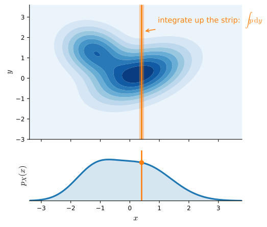
To marginalize, then, we integrate out the variables we do not care about, the same operation introduced in Section 25.4, here given its probabilistic meaning.
27.1.3.2 Conditional Densities and Independence
With the joint and the marginal in hand, the last piece is conditioning: how the density of \(X\) should update once we learn that \(Y=y\). The discrete rule \(P(X\mid Y)=P(X,Y)/P(Y)\) carries over verbatim to densities. We define the conditional density
\[ p_{X\mid Y}(x\mid y) = \frac{p_{X,Y}(x,y)}{p_Y(y)}, \qquad p_Y(y) > 0. \tag{27.1.15}\]
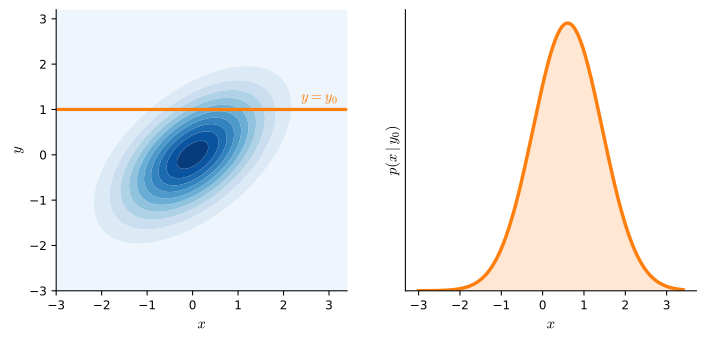
For each fixed \(y\) this is a genuine density in \(x\): it is non-negative, and dividing the joint by exactly \(p_Y(y)=\int p_{X,Y}(x,y)\,dx\) is precisely what makes it integrate to one. Geometrically it is a horizontal slice of the joint surface at height \(y\), renormalized to unit area, as Figure 27.1.6 shows: cut the joint density along \(y=y_0\), then rescale that profile so its area is one. Rearranging Equation 27.1.15 gives the chain rule \(p_{X,Y}(x,y)=p_{X\mid Y}(x\mid y)\,p_Y(y)\), and writing it both ways (\(p_{X,Y}=p_{X\mid Y}\,p_Y=p_{Y\mid X}\,p_X\)) and equating yields Bayes’ rule for densities,
\[ p_{X\mid Y}(x\mid y) = \frac{p_{Y\mid X}(y\mid x)\,p_X(x)}{p_Y(y)}, \tag{27.1.16}\]
which is the identity used for every Bayesian update in this book.
An important special case occurs when the distribution of \(X\) is unchanged after observing \(Y\).
Proposition (independence). The following are equivalent: (i) the joint factorizes, \(p_{X,Y}(x,y)=p_X(x)\,p_Y(y)\) for all \(x,y\); (ii) the conditional equals the marginal, \(p_{X\mid Y}(x\mid y)=p_X(x)\) whenever \(p_Y(y)>0\). When either holds we call \(X\) and \(Y\) independent, \(X\perp Y\).
Proof. If (i) holds, then \(p_{X\mid Y}(x\mid y)=p_X(x)p_Y(y)/p_Y(y)=p_X(x)\), which is (ii). Conversely, if (ii) holds, multiply by \(p_Y(y)\) and use the chain rule: \(p_{X,Y}(x,y)=p_{X\mid Y}(x\mid y)\,p_Y(y)=p_X(x)\,p_Y(y)\), which is (i). \(\blacksquare\)
As a worked example, take the joint \(p_{X,Y}(x,y)=4xy\) on the unit square \([0,1]^2\) (it integrates to one). The marginal is \(p_Y(y)=\int_0^1 4xy\,dx=2y\), so \(p_{X\mid Y}(x\mid y)=4xy/2y=2x\), independent of \(y\). The conditional never changes as \(y\) varies, so by the proposition \(X\perp Y\). This is exactly the visual test of Figure 27.1.6: independence is the case where the renormalized slice \(p(x\mid y_0)\) has the same shape at every height \(y_0\), since the joint factors and the \(y\)-factor cancels in the renormalization. A joint that does not factor this way (say one supported on the triangle \(x\le y\)) has a conditional whose support and shape shift with \(y\), the signature of dependence.
Independence is a strong, all-of-the-distribution statement. It is strictly stronger than being uncorrelated (zero covariance), which constrains only the linear relationship; we make the gap precise in the covariance subsection below. This factorized structure is also exactly what the naive Bayes classifier of Section 27.7 assumes across features to make high-dimensional densities tractable.
27.1.3.3 Conditional Expectation and the Tower Property
The conditional density invites a conditional version of the mean. Averaging \(X\) against the slice \(p_{X\mid Y}(x\mid y)\) rather than its own marginal gives the conditional expectation
\[ E[X\mid Y{=}y] = \int x\,p_{X\mid Y}(x\mid y)\,dx, \tag{27.1.17}\]
the average value of \(X\) once \(Y\) is known to be \(y\). As \(y\) ranges it traces a function of \(y\); feeding in the random \(Y\) makes \(E[X\mid Y]\) itself a random variable, a function of \(Y\) alone. The variance gets a conditional version the same way: \(\textrm{Var}(X\mid Y)=E[X^2\mid Y]-E[X\mid Y]^2\), the computational form Equation 27.1.8 applied within each slice. Two identities then say that conditioning can only reorganize the mean and spread of \(X\), never conjure or destroy them.
Proposition (laws of total expectation and variance). Let \(X,Y\) be jointly continuous with finite variance (for discrete pairs, the same identities hold with every integral replaced by a sum). Then
\[ E[X] = E\bigl[E[X\mid Y]\bigr], \qquad \textrm{Var}(X) = E\bigl[\textrm{Var}(X\mid Y)\bigr] + \textrm{Var}\bigl(E[X\mid Y]\bigr). \tag{27.1.18}\]
Proof. For the first (the tower property), expand the inner expectation and use the chain rule \(p_{X\mid Y}(x\mid y)\,p_Y(y)=p_{X,Y}(x,y)\) to recombine the slices into the joint, then integrate out \(y\) via Equation 27.1.14:
\[ E\bigl[E[X\mid Y]\bigr] = \int\!\Bigl(\int x\,p_{X\mid Y}(x\mid y)\,dx\Bigr)p_Y(y)\,dy = \iint x\,p_{X,Y}(x,y)\,dx\,dy = E[X]. \]
The set where \(p_Y(y)=0\), on which the conditional density Equation 27.1.15 is undefined, contributes nothing to either integral: \(Y\) lands in it with probability zero, and the joint density vanishes there as well (it integrates to \(p_Y\) in \(x\)), so both sides ignore it. For the variance, apply the definition of \(\textrm{Var}(X\mid Y)\) within each slice, take the expectation over \(Y\), and add and subtract \(E\bigl[E[X\mid Y]\bigr]^2=E[X]^2\):
\[ \begin{aligned} E\bigl[\textrm{Var}(X\mid Y)\bigr] + \textrm{Var}\bigl(E[X\mid Y]\bigr) &= \Bigl(E[X^2] - E\bigl[E[X\mid Y]^2\bigr]\Bigr) \\ &\qquad + \Bigl(E\bigl[E[X\mid Y]^2\bigr] - E[X]^2\Bigr) \\ &= E[X^2] - E[X]^2, \end{aligned} \]
which is \(\textrm{Var}(X)\), using the tower property on \(E[X^2]\) and on \(E[X\mid Y]\). \(\blacksquare\)
The variance law (sometimes called Eve’s law, after the E-V-V-E pattern of its right-hand side) has a memorable reading: the spread of \(X\) splits into the average spread within each \(Y\)-slice plus the spread of the slice-averages themselves, unexplained variance plus explained variance. That decomposition underlies the analysis of variance (ANOVA), the classical method that attributes the variation in data to competing explanatory factors, and it reappears in latent-variable models, models that explain observed data through an unobserved cause (Section 27.3.5). We use the tower property Equation 27.1.18 repeatedly when an expectation is easier one slice at a time, most heavily in the maximum-likelihood estimator of Section 27.3 and the variational bounds of Section 28.3.3, where a hidden variable is integrated out one conditional slice at a time.
27.1.3.4 Covariance
For a single extra summary statistic capturing how two variables move together, we use the covariance. For discrete \(X,Y\) taking \((x_i,y_j)\) with probability \(p_{ij}\),
\[\sigma_{XY} = \textrm{Cov}(X, Y) = \sum_{i, j} (x_i - \mu_X)(y_j-\mu_Y)\,p_{ij} = E[XY] - E[X]E[Y], \tag{27.1.19}\]
the second form being the exact two-variable analogue of the computational variance formula Equation 27.1.8 (and indeed \(\textrm{Cov}(X,X)=\textrm{Var}(X)\)). The covariance is positive when \(X\) and \(Y\) tend to be large together, negative when one is large as the other is small.
An example makes this concrete. Let \(X\in\{1,3\}\) and \(Y\in\{-1,3\}\) with
\[ \begin{aligned} P(X{=}1, Y{=}{-}1) &= \tfrac{p}{2}, &\quad P(X{=}1, Y{=}3) &= \tfrac{1-p}{2}, \\ P(X{=}3, Y{=}{-}1) &= \tfrac{1-p}{2}, &\quad P(X{=}3, Y{=}3) &= \tfrac{p}{2}, \end{aligned} \]
for a parameter \(p\in[0,1]\). At \(p=1\) the two are large or small together; at \(p=0\) they are opposed; at \(p=\tfrac12\) all four cells are equally likely and the two are unrelated. With \(\mu_X=2\), \(\mu_Y=1\), the definition Equation 27.1.19 gives, after summing the four terms, \(\textrm{Cov}(X,Y)=4p-2\): equal to \(+2\) at \(p=1\), \(-2\) at \(p=0\), and \(0\) at \(p=\tfrac12\), matching every expectation.
Covariance captures only linear co-variation. If \(Y\) is uniform on \(\{-2,-1,0,1,2\}\) and \(X=Y^2\), then \(X\) is a deterministic function of \(Y\) yet \(\textrm{Cov}(X,Y)=0\), because the symmetric quadratic relationship has no linear trend. Zero covariance does not mean independent.
The continuous version replaces the sum by the density-weighted integral,
\[ \sigma_{XY} = \int_{\mathbb{R}^2} (x-\mu_X)(y-\mu_Y)\,p(x, y)\,dx\,dy . \tag{27.1.20}\]
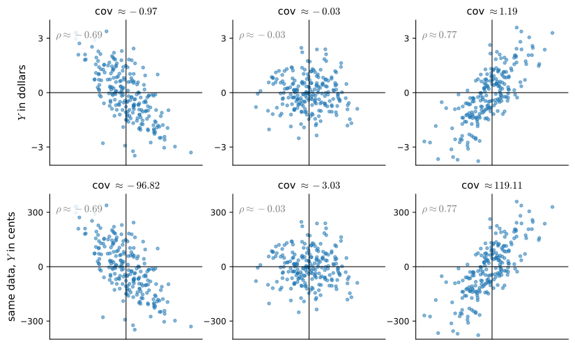
Figure 27.1.7 shows clouds of points whose covariance we tune from negative through zero to positive: the cloud tilts down, rounds out, then tilts up. Its bottom row replays the identical draws with \(Y\) restated in cents instead of dollars: every sample covariance inflates by a factor of \(100\) while no cloud changes shape. Covariance carries the units of its arguments; only its sign is scale-free, a defect the correlation coefficient below will repair.
Two properties we use repeatedly: covariance is linear in each argument, with \(\textrm{Cov}(aX+b,Y)=a\,\textrm{Cov}(X,Y)\) and symmetrically \(\textrm{Cov}(X,cY+d)=c\,\textrm{Cov}(X,Y)\) (shifts drop out, scales pull through, in either slot); and independent variables have zero covariance, since then \(E[XY]=E[X]E[Y]\) in Equation 27.1.19. Covariance also completes the variance-of-a-sum rule.
Proposition (variance of a sum). For any random variables \(X,Y\),
\[ \textrm{Var}(X+Y) = \textrm{Var}(X) + \textrm{Var}(Y) + 2\,\textrm{Cov}(X, Y). \tag{27.1.21}\]
Proof. Write \(\bar X=X-\mu_X\), \(\bar Y=Y-\mu_Y\), so \(X+Y\) has mean \(\mu_X+\mu_Y\) by linearity Equation 27.1.6 and deviation \(\bar X+\bar Y\). Then by Equation 27.1.7 and linearity,
\[ \begin{aligned} \textrm{Var}(X+Y) &= E\bigl[(\bar X+\bar Y)^2\bigr] = E[\bar X^2] + 2\,E[\bar X\bar Y] + E[\bar Y^2] \\ &= \textrm{Var}(X) + 2\,\textrm{Cov}(X,Y) + \textrm{Var}(Y), \end{aligned} \]
recognizing \(E[\bar X\bar Y]=\textrm{Cov}(X,Y)\) from Equation 27.1.19. \(\blacksquare\)
When \(X\) and \(Y\) are independent the cross term vanishes and we recover the additive rule \(\textrm{Var}(X+Y)=\textrm{Var}(X)+\textrm{Var}(Y)\) promised earlier.
27.1.3.5 Correlation
Covariance inherits the units of \(X\) times \(Y\) (inches \(\times\) dollars), so its magnitude is hard to read. Switching \(Y\) from dollars to cents multiplies it by \(100\). To get a unit-free measure, divide by something that also scales by \(100\): the standard deviations. The correlation coefficient is
\[\rho(X, Y) = \frac{\textrm{Cov}(X, Y)}{\sigma_{X}\sigma_{Y}}. \tag{27.1.22}\]
The normalization is calibrated so that \(\rho\) never leaves \([-1,1]\), and the proof is the Cauchy–Schwarz argument of Section 24.1 wearing probabilistic clothes.
Proposition (correlation bound). For any \(X,Y\) with finite, nonzero variances, \(-1\le\rho(X,Y)\le 1\), with equality iff \(Y=aX+b\) almost surely for constants \(a\ne0,b\) (a perfect linear relationship up to probability-zero events).
Proof. A variance is never negative, so \(\textrm{Var}(tX+Y)\ge 0\) for every real \(t\). Expanding it by the variance-of-a-sum rule Equation 27.1.21 (with the affine rule Equation 27.1.9 on the \(tX\) term) gives a quadratic in \(t\),
\[ \textrm{Var}(tX+Y) = \textrm{Var}(X)\,t^2 + 2\,\textrm{Cov}(X,Y)\,t + \textrm{Var}(Y) \;\ge\; 0 \quad\textrm{for every } t. \]
A quadratic with positive leading coefficient \(\textrm{Var}(X)\) that stays non-negative cannot have two distinct real roots, so its discriminant is \(\le 0\):
\[ \bigl(2\,\textrm{Cov}(X,Y)\bigr)^2 - 4\,\textrm{Var}(X)\,\textrm{Var}(Y)\le 0, \qquad\textrm{i.e.}\qquad \textrm{Cov}(X,Y)^2 \le \textrm{Var}(X)\,\textrm{Var}(Y). \]
Dividing by \(\sigma_X^2\sigma_Y^2\) gives \(\rho^2\le 1\), which is the claim. Equality forces the discriminant to vanish, so the quadratic has a (repeated) root \(t^\star\) with \(\textrm{Var}(t^\star X+Y)=0\); a variable of zero variance is constant almost surely, so \(t^\star X+Y=c\) almost surely, i.e. \(Y=-t^\star X+c\) almost surely is affine in \(X\). Conversely, suppose \(Y=aX+b\); the nonzero-variance hypothesis forces \(a\neq0\), since \(a=0\) would make \(Y\) constant. Using \(\textrm{Cov}(X,aX+b)=a\,\textrm{Var}(X)\) (shifts drop out, scales pull through) and \(\sigma_{aX+b}=|a|\sigma_X\),
\[ \rho(X, aX+b) = \frac{a\,\textrm{Var}(X)}{\sigma_X\cdot|a|\,\sigma_X} = \frac{a}{|a|} = \operatorname{sign}(a), \]
so equality holds. \(\blacksquare\)
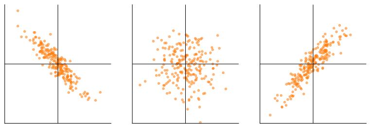
The two extremes thus read off: \(\rho=+1\) for a perfect increasing linear relationship (\(a>0\)) and \(\rho=-1\) for a perfect decreasing one (\(a<0\)), in both cases independent of the scale \(|a|\). Correlation measures the direction and tightness of a linear relationship, never its slope. On the running discrete example \(\sigma_X=1\), \(\sigma_Y=2\), so \(\rho=\frac{4p-2}{2}=2p-1\), sweeping from \(-1\) to \(+1\) as \(p\) does from \(0\) to \(1\). Figure 27.1.8 shows clouds at correlation \(-0.9\), \(0\), and \(0.9\); unlike the covariance clouds, the spread is comparable across panels and only the tilt changes.
There is also a geometric reading. Centering so \(\mu_X=\mu_Y=0\), the correlation Equation 27.1.22 becomes \(\sum_{i,j}x_iy_j\,p_{ij}\) divided by the two root-mean-squares, which is exactly the cosine formula of Section 24.1 with coordinates weighted by \(p_{ij}\). If standard deviations are “lengths” and correlations are “cosines of angles,” that section’s geometric intuition transfers wholesale to random variables: uncorrelated means orthogonal, \(\rho=\pm1\) means parallel.
For \(n\) variables we collect every pairwise covariance into a single covariance matrix \(\boldsymbol\Sigma\) with entries \(\Sigma_{ij}=\textrm{Cov}(X_i,X_j)\), so the diagonal holds the variances and the off-diagonal the cross-terms. It is symmetric because \(\textrm{Cov}\) is. It is also positive semidefinite, by a two-line computation that generalizes the variance-of-a-sum rule Equation 27.1.21: writing \(\bar X_i=X_i-\mu_{X_i}\), the deviation of \(\sum_i a_iX_i\) is \(\sum_i a_i\bar X_i\), and expanding the square inside the expectation,
\[ \textrm{Var}\Bigl(\sum_i a_i X_i\Bigr) = E\Bigl[\Bigl(\sum_i a_i \bar X_i\Bigr)^{\!2}\Bigr] = \sum_{i,j} a_i a_j\,E[\bar X_i \bar X_j] = \sum_{i,j} a_i a_j\,\Sigma_{ij} = \mathbf a^\top \boldsymbol\Sigma\,\mathbf a . \]
The left-hand side is a variance and hence non-negative, so \(\mathbf a^\top\boldsymbol\Sigma\,\mathbf a\ge 0\) for every \(\mathbf a\): positive semidefiniteness is the \(n\)-variable face of \(\textrm{Var}\ge 0\). Because \(\boldsymbol\Sigma\) is symmetric PSD, the spectral theorem (Section 24.2) diagonalizes it. The Gaussian \(\mathcal N(\boldsymbol\mu,\boldsymbol\Sigma)\) is built from exactly this matrix: its density contours are ellipses whose axes point along the eigenvectors of \(\boldsymbol\Sigma\) with half-lengths \(\propto\sqrt{\lambda_i}\), the standard deviation along each principal direction, and we draw and sample these contours when we meet the multivariate Gaussian in Section 27.2 (Figure 27.2.4). Finding those principal axes is principal component analysis, PCA (Section 24.3), and the same deviations-as-vectors geometry underlies least squares Equation 24.1.9.
27.1.3.6 Change of Variables for Densities
One final result closes the section. When we push a random variable through a function \(Y=g(X)\), its density is not generally \(p_X\!\big(g^{-1}(y)\big)\): as the map stretches and compresses space the density must be re-scaled to keep its total mass at \(1\). We already computed the re-scaling factor. The integral change-of-variables theorem of Section 25.4 already established that a reparametrization scales volume locally by the absolute Jacobian determinant, \(\int_{\boldsymbol\phi(U)}f(\mathbf x)\,d\mathbf x=\int_U f(\boldsymbol\phi(\mathbf x))\,|\det D\boldsymbol\phi(\mathbf x)|\,d\mathbf x\) Equation 25.4.9. All a density does is read that theorem with \(f=p\) and the constraint that the total integral stays \(1\): probability mass in equals probability mass out.
Take the one-dimensional case first. Assume that \(g\) is continuously differentiable, one-to-one and monotone on the support of \(X\), with \(g'(x)\ne0\). The intuition is that the mass in a tiny interval must survive the map, \(p_Y(y)\,|dy| = p_X(x)\,|dx|\) with \(y=g(x)\); solving for the new density and writing \(x=g^{-1}(y)\) gives the formula. A derivation needing no infinitesimals takes two lines with tools we already have. For increasing \(g\) the events \(\{g(X)\le y\}\) and \(\{X\le g^{-1}(y)\}\) coincide, so the c.d.f.s satisfy \(F_Y(y)=F_X\bigl(g^{-1}(y)\bigr)\); differentiating with the chain rule and Equation 27.1.4 gives \(p_Y(y)=p_X\bigl(g^{-1}(y)\bigr)\,\tfrac{dg^{-1}}{dy}(y)\), and for decreasing \(g\) the event flips to \(\{X\ge g^{-1}(y)\}\), producing a minus sign that the absolute value absorbs. Either way we obtain the one-dimensional change-of-variables formula
\[ p_Y(y) = p_X\!\big(g^{-1}(y)\big)\,\left|\frac{d g^{-1}}{dy}(y)\right|. \tag{27.1.23}\]
If \(g\) has finitely many regular inverse branches, their contributions add:
\[ p_Y(y)=\sum_{x\in g^{-1}(\{y\})}\frac{p_X(x)}{|g'(x)|}, \]
for values \(y\) whose preimages satisfy \(g'(x)\ne0\). For example, if \(Y=X^2\) and \(y>0\), then \(p_Y(y)=[p_X(\sqrt y)+p_X(-\sqrt y)]/(2\sqrt y)\). Critical points where \(g'(x)=0\), infinitely many inverse branches, and transformations that create atoms require additional analysis.
The derivative factor is exactly the local stretch of the map: where \(g\) spreads a small interval out, the density must drop to keep the area fixed. In several dimensions, assume that \(g\) is a continuously differentiable bijection with a continuously differentiable inverse and nonzero Jacobian determinant. The scalar stretch \(|dg^{-1}/dy|\) becomes the absolute Jacobian determinant, by instantiating Equation 25.4.9 with \(\boldsymbol\phi=g^{-1}\) and \(f=p_X\): \(P(Y\in A)=P\bigl(X\in g^{-1}(A)\bigr)=\int_{g^{-1}(A)}p_X(\mathbf x)\,d\mathbf x =\int_A p_X\bigl(g^{-1}(\mathbf y)\bigr)\,\bigl|\det J_{g^{-1}}(\mathbf y)\bigr|\,d\mathbf y\), so the integrand on the right is the density of \(Y\). Conservation of mass thus reads
\[ \begin{aligned} p_Y(\mathbf y) &= p_X\!\big(g^{-1}(\mathbf y)\big)\,\big|\det J_{g^{-1}}(\mathbf y)\big|, \\ \text{equivalently}\qquad \log p_Y(\mathbf y) &= \log p_X(\mathbf x) - \log\big|\det J_{g}(\mathbf x)\big| \quad\text{at }\mathbf x = g^{-1}(\mathbf y). \end{aligned} \tag{27.1.24}\]
The logarithmic form is convenient in practice. Passing data through an invertible network adds \(-\log|\det J_g|\) to the log-density. Because \(\log|\det(J_2 J_1)| = \log|\det J_1| + \log|\det J_2|\), a composition of layers contributes the sum of their log-determinants. This additivity permits efficient likelihood evaluation in normalizing flows (Rezende and Mohamed 2015) (Section 29.1.5).
As a worked example, let \(X\sim\mathcal N(0,1)\) and \(Y=e^X\), so \(g^{-1}(y)=\log y\) and \(|dg^{-1}/dy| = 1/y\) for \(y>0\). Formula Equation 27.1.23 gives the log-normal density
\[ p_Y(y) = \frac{1}{y\sqrt{2\pi}}\,\exp\!\Big(-\tfrac12(\log y)^2\Big), \qquad y>0, \]
whose \(1/y\) prefactor is precisely the change-of-variables correction. The prediction is directly checkable: sample \(X\sim\mathcal N(0,1)\), push the samples through \(e^X\), and a histogram of the results should trace out this density, \(1/y\) correction and all.
# Push X ~ N(0, 1) through Y = e^X and compare a histogram of the samples
# with the log-normal density predicted by the change-of-variables formula
np.random.seed(0)
y = np.exp(np.random.randn(100000))
edges = np.linspace(0.0, 8.0, 65)
mids, width = (edges[:-1] + edges[1:]) / 2, edges[1] - edges[0]
hist = np.histogram(y, edges)[0] / (100000 * width)
analytic = np.exp(-np.log(mids)**2 / 2) / (mids * np.sqrt(2 * np.pi))
d2l.plot(mids, [hist, analytic], 'y', 'p(y)',
         legend=['histogram of exp(X)', 'log-normal density'])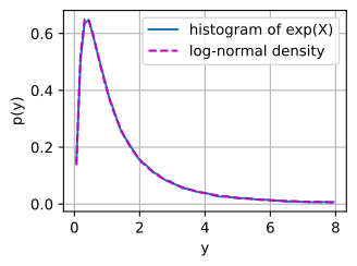
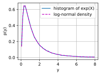
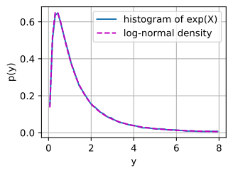
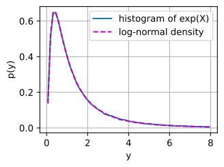
The two curves coincide: the mass pushed forward through \(e^x\) piles up exactly where Equation 27.1.23 says it must, including the mode at \(y=e^{-1}\). The naive guess \(p_X(\log y)\) gets that mode wrong, peaking at \(y=1\) instead. A linear map \(\mathbf y = A\mathbf x\) illustrates the multivariate rule in one stroke: \(J_g=A\) is constant, so the density is rescaled uniformly by \(1/|\det A|\); stretch space by \(|\det A|\) and the density thins by the same factor.
27.1.4 Summary
- A continuous random variable is described by a probability density \(p(x)\ge0\) with \(\int p\,dx=1\) Equation 25.4.11; the density is not itself a probability; only its integral over an interval is, \(P(X\in(a,b])=\int_a^b p\) Equation 27.1.2. Any single point, and more generally any set of measure zero (coverable by intervals of arbitrarily small total length), has probability zero.
- The cumulative distribution function \(F(x)=\int_{-\infty}^x p=P(X\le x)\) is a probability and unifies discrete, continuous, and mixed variables. Density and c.d.f. are derivative and integral of each other: \(F'=p\) Equation 27.1.4, the fundamental theorem of calculus.
- The mean \(\mu_X=E[X]\) locates the distribution and is linear Equation 27.1.6: sums of expectations add with no independence needed. The variance \(\textrm{Var}(X)=E[X^2]-\mu_X^2\) Equation 27.1.8 measures spread, scales as \(\textrm{Var}(aX+b)=a^2\textrm{Var}(X)\) Equation 27.1.9, and its root is the standard deviation, back in the original units.
- Markov’s inequality Equation 27.1.11 caps the tail of a non-negative variable by its mean; applied to \((X-\mu_X)^2\) it yields Chebyshev’s inequality Equation 27.1.12: at most a \(1/\alpha^2\) fraction of any distribution lies \(\alpha\) standard deviations or farther from the mean.
- Several variables are handled by a joint density; marginals come from integrating out the unwanted variables Equation 27.1.14. Covariance measures linear co-variation, giving \(\textrm{Var}(X+Y)=\textrm{Var}(X)+ \textrm{Var}(Y)+2\textrm{Cov}(X,Y)\) Equation 27.1.21, and correlation normalizes it to \([-1,1]\) as a cosine between centered variables. Zero covariance does not imply independence.
- Pushing \(X\) through an invertible map \(g\) rescales its density by the local stretch of the map: \(p_Y(y)=p_X(g^{-1}(y))\,|dg^{-1}/dy|\) Equation 27.1.23, with the absolute Jacobian determinant taking over in several dimensions Equation 27.1.24, the log-det form that powers normalizing flows.
27.1.5 Exercises
- Suppose \(X\) has density \(p(x) = \frac{1}{x^2}\) for \(x \ge 1\) and \(p(x) = 0\) otherwise. Verify it is a density and compute \(P(X > 2)\) and the c.d.f. \(F(x)\).
- The Laplace distribution has density \(p(x) = \tfrac12 e^{-|x|}\). Find its mean and standard deviation. (Hint: \(\int_0^\infty xe^{-x}\,dx = 1\) and \(\int_0^\infty x^2e^{-x}\,dx = 2\).)
- A population has mean \(1\) and standard deviation \(2\). Use Chebyshev Equation 27.1.12 to bound the population probability \(P(X>9)\). Then explain why observing \(25\%\) above \(9\) in a finite sample is evidence against the claim but is not logically impossible without knowing the sample size.
- Two variables \(X,Y\) have joint density \(p_{XY}(x, y) = x+y\) on \([0,1]^2\) and \(0\) otherwise. Verify that it integrates to one, find the marginals \(p_X,p_Y\) and the covariance \(\textrm{Cov}(X,Y)\), and decide whether \(X\) and \(Y\) are independent.
- Give a second proof of the affine variance rule \(\textrm{Var}(aX+b)=a^2\textrm{Var}(X)\) Equation 27.1.9, this time starting from the computational form \(\textrm{Var}(aX+b)=E[(aX+b)^2]-E[aX+b]^2\) Equation 27.1.8: expand both expectations with linearity Equation 27.1.6 and watch the cross terms cancel. (The proof in the text instead worked with the deviation \(a(X-\mu_X)\).)
- Using \(\textrm{Var}(X+Y)=\textrm{Var}(X)+\textrm{Var}(Y)+2\textrm{Cov}(X,Y)\) Equation 27.1.21, show that for independent identically distributed \(X_1,\ldots,X_n\) with variance \(\sigma^2\), the sample mean \(\bar X=\tfrac1n\sum_i X_i\) has variance \(\sigma^2/n\). (This is why averaging reduces noise.)
- Let \(X\) be uniform on \(\{-1,0,1\}\) and \(Y=|X|\). Compute \(\textrm{Cov}(X,Y)\) and confirm it is zero even though \(Y\) is a deterministic function of \(X\). Why does correlation miss this relationship?