from d2l import torch as d2l
import torch
import torchvision
from torch import nn
import os20.14 Dog Breed Identification (ImageNet Dogs) on Kaggle
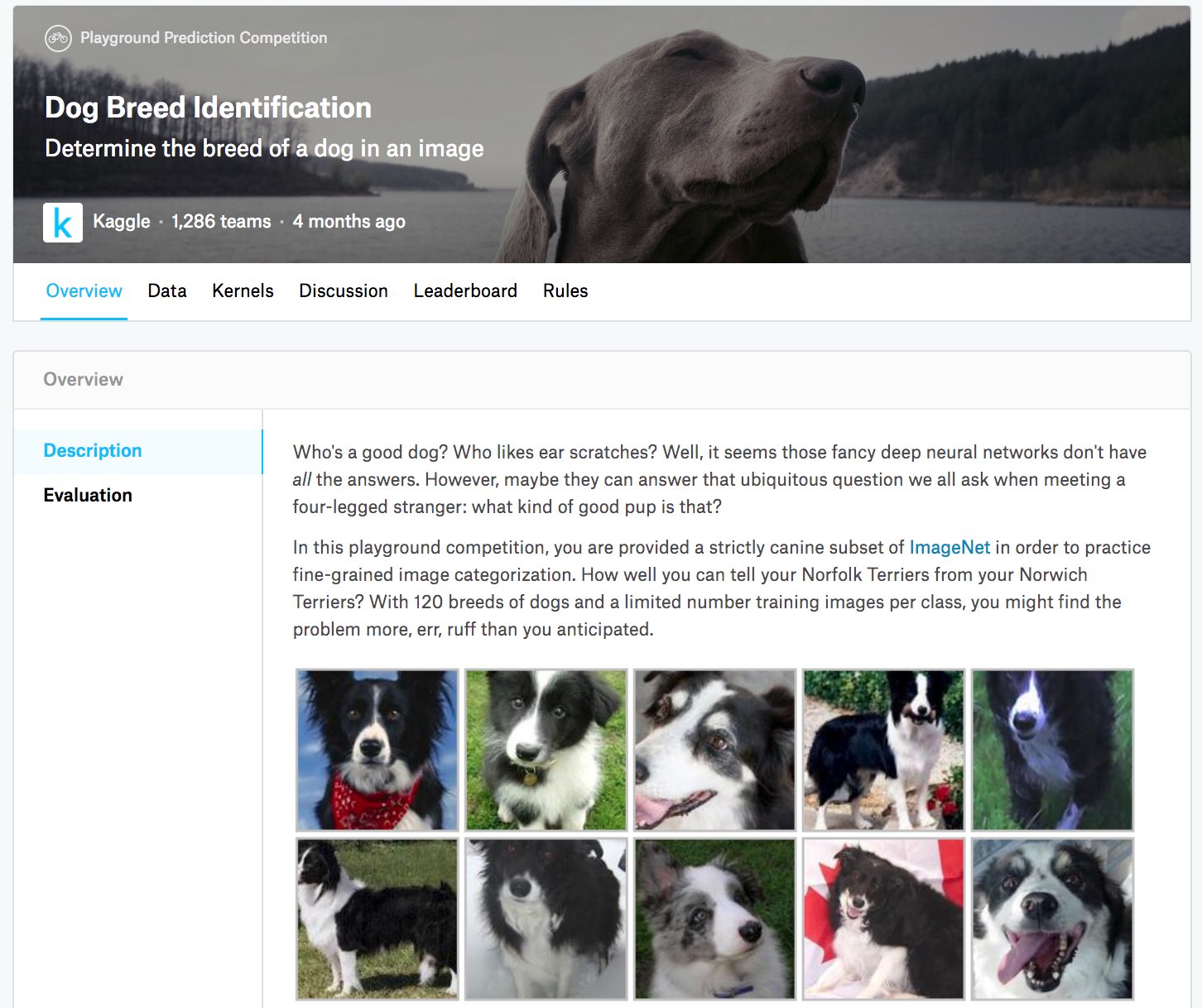
In this section, we will practice the dog breed identification problem on Kaggle. The web address of this competition is https://www.kaggle.com/c/dog-breed-identification
In this competition, 120 different breeds of dogs will be recognized. In fact, the dataset for this competition is a subset of the ImageNet dataset. Unlike the images in the CIFAR-10 dataset in Section 20.13, the images in the ImageNet dataset are both higher and wider in varying dimensions. Figure 20.14.1 shows the information on the competition’s webpage. You need a Kaggle account to submit your results.
from d2l import tensorflow as d2l
import tensorflow as tf
import keras
import numpy as np
import os
from d2l import jax as d2l
import jax
from jax import numpy as jnp
from flax import nnx
import optax
import numpy as np
from d2l.nnx_resnet import ResNet50
import tensorflow as tf # data pipeline only (tf.data); all compute runs in JAX
import osfrom d2l import mxnet as d2l
from mxnet import autograd, gluon, init, npx
from mxnet.gluon import nn
import os
npx.set_np()20.14.1 Obtaining and Organizing the Dataset
The competition dataset is divided into a training set and a test set, which contain 10222 and 10357 JPEG images of three RGB (color) channels, respectively. Among the training dataset, there are 120 breeds of dogs such as Labradors, Poodles, Dachshunds, Samoyeds, Huskies, Chihuahuas, and Yorkshire Terriers.
20.14.1.1 Downloading the Dataset
After logging into Kaggle, you can click on the “Data” tab on the competition webpage shown in Figure 20.14.1 and download the dataset by clicking the “Download All” button. After unzipping the downloaded file in ../data, you will find the entire dataset in the following paths:
- ../data/dog-breed-identification/labels.csv
- ../data/dog-breed-identification/sample_submission.csv
- ../data/dog-breed-identification/train
- ../data/dog-breed-identification/test
You may have noticed that the above structure is similar to that of the CIFAR-10 competition in Section 20.13, where folders train/ and test/ contain training and testing dog images, respectively, and labels.csv contains the labels for the training images. Similarly, to make it easier to get started, we provide a small sample of the dataset mentioned above: train_valid_test_tiny.zip. If you are going to use the full dataset for the Kaggle competition, you need to change the demo variable below to False.
d2l.DATA_HUB['dog_tiny'] = (d2l.DATA_URL + 'kaggle_dog_tiny.zip',
                            '0cb91d09b814ecdc07b50f31f8dcad3e81d6a86d')

# If you use the full dataset downloaded for the Kaggle competition, change
# the variable below to `False`
demo = True
if demo:
    data_dir = d2l.download_extract('dog_tiny')
else:
    data_dir = os.path.join('..', 'data', 'dog-breed-identification')
20.14.1.2 Organizing the Dataset
We can organize the dataset similarly to what we did in Section 20.13, namely splitting out a validation set from the original training set, and moving images into subfolders grouped by labels.
The reorg_dog_data function below reads the training data labels, splits out the validation set, and organizes the training set.
def reorg_dog_data(data_dir, valid_ratio):
    labels = d2l.read_csv_labels(os.path.join(data_dir, 'labels.csv'))
    d2l.reorg_train_valid(data_dir, labels, valid_ratio)
    d2l.reorg_test(data_dir)


batch_size = 32 if demo else 128
valid_ratio = 0.1
reorg_dog_data(data_dir, valid_ratio)
20.14.2 Image Augmentation
Recall that this dog breed dataset is a subset of the ImageNet dataset, whose images are larger than those of the CIFAR-10 dataset in Section 20.13. The following lists a few image augmentation operations that might be useful for relatively larger images.
transform_train = torchvision.transforms.Compose([
    # Randomly crop the image to obtain an image with an area of 0.08 to 1 of
    # the original area and height-to-width ratio between 3/4 and 4/3. Then,
    # scale the image to create a new 224 x 224 image
    torchvision.transforms.RandomResizedCrop(224, scale=(0.08, 1.0),
                                             ratio=(3.0/4.0, 4.0/3.0)),
    torchvision.transforms.RandomHorizontalFlip(),
    # Randomly change the brightness, contrast, and saturation
    torchvision.transforms.ColorJitter(brightness=0.4,
                                       contrast=0.4,
                                       saturation=0.4),
    # Add random noise
    torchvision.transforms.ToTensor(),
    # Standardize each channel of the image
    torchvision.transforms.Normalize([0.485, 0.456, 0.406],
                                     [0.229, 0.224, 0.225])])
def transform_train_fn(image, label):
"""Training augmentation: random crop, flip, color jitter, normalize."""
image = tf.cast(image, tf.float32)
# Random resized crop to 224x224
image = tf.image.resize(image, [256, 256])
image = tf.image.random_crop(image, size=[224, 224, 3])
image = tf.image.random_flip_left_right(image)
image = tf.image.random_brightness(image, max_delta=0.4 * 255)
image = tf.image.random_contrast(image, lower=0.6, upper=1.4)
image = tf.image.random_saturation(image, lower=0.6, upper=1.4)
image = tf.clip_by_value(image, 0.0, 255.0)
return tf.keras.applications.resnet50.preprocess_input(image), labelIMAGENET_MEAN = tf.constant([0.485, 0.456, 0.406], tf.float32)
IMAGENET_STD = tf.constant([0.229, 0.224, 0.225], tf.float32)
def transform_train_fn(image, label):
"""Training augmentation followed by ImageNet normalization."""
image = tf.cast(image, tf.float32)
# Random resized crop to 224x224
image = tf.image.resize(image, [256, 256])
image = tf.image.random_crop(image, size=[224, 224, 3])
image = tf.image.random_flip_left_right(image)
image = tf.image.random_brightness(image, max_delta=0.4 * 255)
image = tf.image.random_contrast(image, lower=0.6, upper=1.4)
image = tf.image.random_saturation(image, lower=0.6, upper=1.4)
image = tf.clip_by_value(image, 0.0, 255.0)
image = image / 255.0
return (image - IMAGENET_MEAN) / IMAGENET_STD, labeltransform_train = gluon.data.vision.transforms.Compose([
# Randomly crop the image to obtain an image with an area of 0.08 to 1 of
# the original area and height-to-width ratio between 3/4 and 4/3. Then,
# scale the image to create a new 224 x 224 image
gluon.data.vision.transforms.RandomResizedCrop(224, scale=(0.08, 1.0),
ratio=(3.0/4.0, 4.0/3.0)),
gluon.data.vision.transforms.RandomFlipLeftRight(),
# Randomly change the brightness, contrast, and saturation
gluon.data.vision.transforms.RandomColorJitter(brightness=0.4,
contrast=0.4,
saturation=0.4),
# Add random noise
gluon.data.vision.transforms.RandomLighting(0.1),
gluon.data.vision.transforms.ToTensor(),
# Standardize each channel of the image
gluon.data.vision.transforms.Normalize([0.485, 0.456, 0.406],
[0.229, 0.224, 0.225])])During prediction, we only use image preprocessing operations without randomness.
transform_test = torchvision.transforms.Compose([
    torchvision.transforms.Resize(256),
    # Crop a 224 x 224 square area from the center of the image
    torchvision.transforms.CenterCrop(224),
    torchvision.transforms.ToTensor(),
    torchvision.transforms.Normalize([0.485, 0.456, 0.406],
                                     [0.229, 0.224, 0.225])])
def transform_test_fn(image, label):
"""Test preprocessing: resize, center crop, normalize."""
image = tf.cast(image, tf.float32)
image = tf.image.resize(image, [256, 256])
# Center crop to 224x224
image = tf.image.resize_with_crop_or_pad(image, 224, 224)
return tf.keras.applications.resnet50.preprocess_input(image), labeldef transform_test_fn(image, label):
"""Test preprocessing: resize, center crop, and normalize."""
image = tf.cast(image, tf.float32)
image = tf.image.resize(image, [256, 256])
# Center crop to 224x224
image = tf.image.resize_with_crop_or_pad(image, 224, 224)
image = image / 255.0
return (image - IMAGENET_MEAN) / IMAGENET_STD, labeltransform_test = gluon.data.vision.transforms.Compose([
gluon.data.vision.transforms.Resize(256),
# Crop a 224 x 224 square area from the center of the image
gluon.data.vision.transforms.CenterCrop(224),
gluon.data.vision.transforms.ToTensor(),
gluon.data.vision.transforms.Normalize([0.485, 0.456, 0.406],
[0.229, 0.224, 0.225])])20.14.3 Reading the Dataset
As in Section 20.13, we can read the organized dataset consisting of raw image files.
train_ds, train_valid_ds = [torchvision.datasets.ImageFolder(
    os.path.join(data_dir, 'train_valid_test', folder),
    transform=transform_train) for folder in ['train', 'train_valid']]

valid_ds, test_ds = [torchvision.datasets.ImageFolder(
    os.path.join(data_dir, 'train_valid_test', folder),
    transform=transform_test) for folder in ['valid', 'test']]
def _load_image_folder_tf(folder_path):
"""Load images from a class-subfolder directory into a tf.data.Dataset."""
ds = keras.utils.image_dataset_from_directory(
folder_path, label_mode='int', image_size=(256, 256),
batch_size=None, shuffle=False)
return ds
train_ds = _load_image_folder_tf(
os.path.join(data_dir, 'train_valid_test', 'train'))
train_valid_ds = _load_image_folder_tf(
os.path.join(data_dir, 'train_valid_test', 'train_valid'))
valid_ds = _load_image_folder_tf(
os.path.join(data_dir, 'train_valid_test', 'valid'))
test_ds = _load_image_folder_tf(
os.path.join(data_dir, 'train_valid_test', 'test'))Found 880 files belonging to 120 classes.
Found 1000 files belonging to 120 classes.
Found 120 files belonging to 120 classes.
Found 10 files belonging to 1 classes.def _load_image_folder_tf(folder_path):
"""Load images from a class-subfolder directory into a tf.data.Dataset."""
ds = tf.keras.utils.image_dataset_from_directory(
folder_path, label_mode='int', image_size=(256, 256),
batch_size=None, shuffle=False)
return ds
train_ds = _load_image_folder_tf(
os.path.join(data_dir, 'train_valid_test', 'train'))
train_valid_ds = _load_image_folder_tf(
os.path.join(data_dir, 'train_valid_test', 'train_valid'))
valid_ds = _load_image_folder_tf(
os.path.join(data_dir, 'train_valid_test', 'valid'))
test_ds = _load_image_folder_tf(
os.path.join(data_dir, 'train_valid_test', 'test'))Found 880 files belonging to 120 classes.
Found 1000 files belonging to 120 classes.
Found 120 files belonging to 120 classes.
Found 10 files belonging to 1 classes.train_ds, valid_ds, train_valid_ds, test_ds = [
gluon.data.vision.ImageFolderDataset(
os.path.join(data_dir, 'train_valid_test', folder))
for folder in ('train', 'valid', 'train_valid', 'test')]Below we create data iterator instances the same way as in Section 20.13.
train_iter, train_valid_iter = [torch.utils.data.DataLoader(
    dataset, batch_size, shuffle=True, drop_last=True)
    for dataset in (train_ds, train_valid_ds)]

valid_iter = torch.utils.data.DataLoader(valid_ds, batch_size, shuffle=False,
                                         drop_last=True)

test_iter = torch.utils.data.DataLoader(test_ds, batch_size, shuffle=False,
                                        drop_last=False)
train_iter = (train_ds.map(transform_train_fn, num_parallel_calls=tf.data.AUTOTUNE)
.shuffle(10000).batch(batch_size, drop_remainder=True)
.prefetch(tf.data.AUTOTUNE))
train_valid_iter = (train_valid_ds.map(transform_train_fn,
num_parallel_calls=tf.data.AUTOTUNE)
.shuffle(10000).batch(batch_size, drop_remainder=True)
.prefetch(tf.data.AUTOTUNE))
valid_iter = (valid_ds.map(transform_test_fn, num_parallel_calls=tf.data.AUTOTUNE)
.batch(batch_size, drop_remainder=True)
.prefetch(tf.data.AUTOTUNE))
test_iter = (test_ds.map(transform_test_fn, num_parallel_calls=tf.data.AUTOTUNE)
.batch(batch_size, drop_remainder=False)
.prefetch(tf.data.AUTOTUNE))train_iter = (train_ds.map(transform_train_fn, num_parallel_calls=tf.data.AUTOTUNE)
.shuffle(10000).batch(batch_size, drop_remainder=True)
.prefetch(tf.data.AUTOTUNE))
train_valid_iter = (train_valid_ds.map(transform_train_fn,
num_parallel_calls=tf.data.AUTOTUNE)
.shuffle(10000).batch(batch_size, drop_remainder=True)
.prefetch(tf.data.AUTOTUNE))
valid_iter = (valid_ds.map(transform_test_fn, num_parallel_calls=tf.data.AUTOTUNE)
.batch(batch_size, drop_remainder=True)
.prefetch(tf.data.AUTOTUNE))
test_iter = (test_ds.map(transform_test_fn, num_parallel_calls=tf.data.AUTOTUNE)
.batch(batch_size, drop_remainder=False)
.prefetch(tf.data.AUTOTUNE))train_iter, train_valid_iter = [gluon.data.DataLoader(
dataset.transform_first(transform_train), batch_size, shuffle=True,
last_batch='discard') for dataset in (train_ds, train_valid_ds)]
valid_iter = gluon.data.DataLoader(
valid_ds.transform_first(transform_test), batch_size, shuffle=False,
last_batch='discard')
test_iter = gluon.data.DataLoader(
test_ds.transform_first(transform_test), batch_size, shuffle=False,
last_batch='keep')20.14.4 Fine-Tuning a Pretrained Model
Again, the dataset for this competition is a subset of the ImageNet dataset. Therefore, we can use the approach discussed in Section 20.2 to select a model pretrained on the full ImageNet dataset and use it to extract image features to be fed into a custom small-scale output network. High-level APIs of deep learning frameworks provide a wide range of models pretrained on the ImageNet dataset. Here, we choose a pretrained ResNet-34 model, where we simply reuse the input of this model’s output layer (i.e., the extracted features). Then we can replace the original output layer with a small custom output network that can be trained, such as stacking two fully connected layers. Different from the experiment in Section 20.2, the following does not retrain the pretrained model used for feature extraction. This reduces training time and memory for storing gradients.
Recall that we standardized images using the means and standard deviations of the three RGB channels for the full ImageNet dataset. In fact, this is also consistent with the standardization operation by the pretrained model on ImageNet.
def get_net(devices):
    finetune_net = nn.Sequential()
    finetune_net.features = torchvision.models.resnet34(
        weights=torchvision.models.ResNet34_Weights.DEFAULT)
    # Define a new output network (there are 120 output categories)
    finetune_net.output_new = nn.Sequential(nn.Linear(1000, 256),
                                            nn.ReLU(),
                                            nn.Linear(256, 120))
    # Move the model to devices
    finetune_net = finetune_net.to(devices[0])
    # Freeze parameters of feature layers
    for param in finetune_net.features.parameters():
        param.requires_grad = False
    return finetune_net
# Frozen ImageNet ResNet-50 feature extractor plus a small trainable 120-way
# head. We keep them as SEPARATE models (not one Keras `Model`) so the frozen
# backbone can run OUTSIDE the GradientTape and in micro-batches: a batch-32
# ResNet-50 forward at 224x224 otherwise reserves ~8.6 GiB (its activations are
# held for the head's backprop), whereas the JAX/PyTorch tabs never retain the
# backbone activations. Micro-batching caps the peak activation working set.
BACKBONE_MICROBATCH = 16
def get_net():
backbone = keras.applications.ResNet50(
weights='imagenet', include_top=True, classifier_activation=None,
input_shape=(224, 224, 3))
backbone.trainable = False
head = keras.Sequential([keras.layers.Input(shape=(1000,)),
keras.layers.Dense(256, activation='relu'),
keras.layers.Dense(120)])
return backbone, head
def backbone_features(backbone, X):
"""Run the frozen backbone in micro-batches. The concatenated result is
identical to a single forward pass, but only one micro-batch's activations
are live at a time, so the peak footprint stays small."""
outs = [backbone(X[i:i + BACKBONE_MICROBATCH], training=False)
for i in range(0, X.shape[0], BACKBONE_MICROBATCH)]
return tf.concat(outs, axis=0)# Frozen ImageNet-pretrained NNX ResNet-50. We train a small dog-breed head on
# its pooled 2048-dimensional features.
class OutputNet(nnx.Module):
"""Small output network for fine-tuning."""
def __init__(self, num_classes=120, *, rngs):
self.layers = nnx.Sequential(
nnx.Linear(2048, 256, rngs=rngs), nnx.relu,
nnx.Linear(256, num_classes, rngs=rngs))
def __call__(self, x):
return self.layers(x)
def get_net():
backbone = ResNet50.from_pretrained()
output_net = OutputNet(num_classes=120, rngs=nnx.Rngs(1))
return backbone, output_netdef get_net(devices):
finetune_net = gluon.model_zoo.vision.resnet34_v2(pretrained=True)
# Define a new output network
finetune_net.output_new = nn.HybridSequential()
finetune_net.output_new.add(nn.Dense(256, activation='relu'))
# There are 120 output categories
finetune_net.output_new.add(nn.Dense(120))
# Initialize the output network
finetune_net.output_new.initialize(init.Xavier(), ctx=devices)
# Distribute the model parameters to the CPUs or GPUs used for computation
finetune_net.reset_ctx(devices)
return finetune_netBefore calculating the loss, we first obtain the input of the pretrained model’s output layer, i.e., the extracted feature. Then we use this feature as input for our small custom output network to calculate the loss.
loss = nn.CrossEntropyLoss(reduction='none')

def evaluate_loss(data_iter, net, devices):
    l_sum, n = 0.0, 0
    for features, labels in data_iter:
        features, labels = features.to(devices[0]), labels.to(devices[0])
        outputs = net(features)
        l = loss(outputs, labels)
        l_sum += l.sum()
        n += labels.numel()
    return l_sum / n
loss = keras.losses.SparseCategoricalCrossentropy(
from_logits=True, reduction='none')
def evaluate_loss(data_iter, backbone, head):
l_sum, n = 0.0, 0
for features, labels in data_iter:
logits = head(backbone_features(backbone, features), training=False)
l = loss(labels, logits)
l_sum += float(tf.reduce_sum(l))
n += len(labels)
return l_sum / ndef loss_fn(logits, labels):
return optax.softmax_cross_entropy_with_integer_labels(logits, labels)
@nnx.jit
def extract_features(backbone, X_batch):
"""Frozen ResNet-50 forward (on GPU) -> pooled 2048-d features."""
return backbone.features(jnp.asarray(X_batch))
def precompute_features(backbone, data_iter):
"""Run the frozen backbone (on GPU) over the whole dataset and cache the
(features, labels) tensors as JAX arrays. Subsequent training only
iterates the small classifier head over these cached features."""
feats_list, labels_list = [], []
for features, labels in data_iter:
f = extract_features(backbone, features.numpy())
feats_list.append(np.asarray(f))
labels_list.append(labels.numpy())
feats = jnp.array(np.concatenate(feats_list, axis=0))
labels = jnp.array(np.concatenate(labels_list, axis=0))
return feats, labels
def evaluate_loss_from_feats(feats, labels, output_net, batch_size):
l_sum, n = 0.0, 0
for i in range(0, feats.shape[0], batch_size):
fb = feats[i:i + batch_size]
yb = labels[i:i + batch_size]
logits = output_net(fb)
l = loss_fn(logits, yb)
l_sum += float(l.sum())
n += int(yb.shape[0])
return l_sum / nloss = gluon.loss.SoftmaxCrossEntropyLoss()
def evaluate_loss(data_iter, net, devices):
l_sum, n = 0.0, 0
for features, labels in data_iter:
X_shards, y_shards = d2l.split_batch(features, labels, devices)
output_features = [net.features(X_shard) for X_shard in X_shards]
outputs = [net.output_new(feature) for feature in output_features]
ls = [loss(output, y_shard).sum() for output, y_shard
in zip(outputs, y_shards)]
l_sum += sum([float(l.sum()) for l in ls])
n += labels.size
return l_sum / n20.14.5 Defining the Training Function
We will select the model and tune hyperparameters according to the model’s performance on the validation set. The model training function train only iterates parameters of the small custom output network.
def train(net, train_iter, valid_iter, num_epochs, lr, wd, devices, lr_period,
          lr_decay):
    # Only train the small custom output network
    net = nn.DataParallel(net, device_ids=devices).to(devices[0])
    trainer = torch.optim.SGD((param for param in net.parameters()
                               if param.requires_grad), lr=lr,
                              momentum=0.9, weight_decay=wd)
    scheduler = torch.optim.lr_scheduler.StepLR(trainer, lr_period, lr_decay)
    num_batches, timer = len(train_iter), d2l.Timer()
    legend = ['train loss']
    if valid_iter is not None:
        legend.append('valid loss')
    animator = d2l.Animator(xlabel='epoch', xlim=[1, num_epochs],
                            legend=legend)
    for epoch in range(num_epochs):
        metric = d2l.Accumulator(2)
        for i, (features, labels) in enumerate(train_iter):
            timer.start()
            features, labels = features.to(devices[0]), labels.to(devices[0])
            trainer.zero_grad()
            output = net(features)
            l = loss(output, labels).sum()
            l.backward()
            trainer.step()
            metric.add(l, labels.shape[0])
            timer.stop()
            if (i + 1) % (num_batches // 5) == 0 or i == num_batches - 1:
                animator.add(epoch + (i + 1) / num_batches,
                             (metric[0] / metric[1], None))
        measures = f'train loss {metric[0] / metric[1]:.3f}'
        if valid_iter is not None:
            valid_loss = evaluate_loss(valid_iter, net, devices)
            animator.add(epoch + 1, (None, valid_loss.detach().cpu()))
        scheduler.step()
    if valid_iter is not None:
        measures += f', valid loss {valid_loss:.3f}'
    print(measures + f'\n{metric[1] * num_epochs / timer.sum():.1f}'
          f' examples/sec on {str(devices)}')
def train(backbone, head, train_iter, valid_iter, num_epochs, lr, wd,
lr_period, lr_decay):
# Only train the custom head; the backbone is frozen (see get_net()) and is
# run outside the tape.
# Keras's `ExponentialDecay.decay_steps` counts *gradient-update
# steps*, not epochs — unlike PyTorch's `StepLR(step_size=lr_period)`,
# which the PT tab steps once per epoch. Scale by `num_batches` so the
# LR decays every `lr_period` *epochs*, matching PT/MX.
num_batches = sum(1 for _ in train_iter)
lr_schedule = keras.optimizers.schedules.ExponentialDecay(
initial_learning_rate=lr,
decay_steps=lr_period * num_batches,
decay_rate=lr_decay,
staircase=True)
optimizer = keras.optimizers.SGD(learning_rate=lr_schedule, momentum=0.9,
weight_decay=wd)
timer = d2l.Timer()
legend = ['train loss']
if valid_iter is not None:
legend.append('valid loss')
animator = d2l.Animator(xlabel='epoch', xlim=[1, num_epochs],
legend=legend)
for epoch in range(num_epochs):
metric = d2l.Accumulator(2)
for i, (features, labels) in enumerate(train_iter):
timer.start()
# Frozen backbone forward runs outside the tape (its activations are
# freed immediately); only the small head is taped for backprop.
feats = backbone_features(backbone, features)
with tf.GradientTape() as tape:
logits = head(feats, training=True)
l = loss(labels, logits)
grads = tape.gradient(l, head.trainable_variables)
optimizer.apply_gradients(zip(grads, head.trainable_variables))
metric.add(float(tf.reduce_sum(l)), len(labels))
timer.stop()
if (i + 1) % (num_batches // 5) == 0 or i == num_batches - 1:
animator.add(epoch + (i + 1) / num_batches,
(metric[0] / metric[1], None))
measures = f'train loss {metric[0] / metric[1]:.3f}'
if valid_iter is not None:
valid_loss = evaluate_loss(valid_iter, backbone, head)
animator.add(epoch + 1, (None, valid_loss))
if valid_iter is not None:
measures += f', valid loss {valid_loss:.3f}'
print(measures + f'\n{metric[1] * num_epochs / timer.sum():.1f}'
f' examples/sec')
return headdef train(backbone, output_net, train_iter, valid_iter,
num_epochs, lr, wd, lr_period, lr_decay):
# Only train the small custom output network
timer = d2l.Timer()
legend = ['train loss']
if valid_iter is not None:
legend.append('valid loss')
animator = d2l.Animator(xlabel='epoch', xlim=[1, num_epochs],
legend=legend)
# Run the frozen TF backbone over the training set once to determine
# n_train and num_batches, which are needed to configure the LR schedule
# before the epoch loop starts.
print('Pre-extracting train features...')
train_feats, train_labels = precompute_features(backbone, train_iter)
if valid_iter is not None:
print('Pre-extracting valid features...')
valid_feats, valid_labels = precompute_features(backbone, valid_iter)
# Use the same batch size as the data loader (defined globally).
bs = batch_size
n_train = int(train_feats.shape[0])
num_batches = (n_train + bs - 1) // bs
# `optax.exponential_decay.transition_steps` counts *gradient-update
# steps*, not epochs — unlike PyTorch's `StepLR(step_size=lr_period)`,
# which the PT tab steps once per epoch. Scale by `num_batches` so the
# LR decays every `lr_period` *epochs*, matching PT/MX.
schedule = optax.exponential_decay(
init_value=lr, transition_steps=lr_period * num_batches,
decay_rate=lr_decay, staircase=True)
tx = optax.chain(optax.add_decayed_weights(wd),
optax.sgd(schedule, momentum=0.9))
optimizer = nnx.Optimizer(output_net, tx, wrt=nnx.Param)
@nnx.jit
def train_step(output_net, optimizer, feats, y):
def compute_loss(output_net):
logits = output_net(feats)
l = loss_fn(logits, y)
# Backprop on the per-batch *sum* (not mean) to match the PT/TF
# tabs, which use reduction='none' + .sum(). Otherwise the
# effective learning rate here is 1/batch_size smaller and the
# head barely moves.
s = l.sum()
return s
l_sum, grads = nnx.value_and_grad(compute_loss)(output_net)
optimizer.update(output_net, grads)
return l_sum
rng = np.random.default_rng(0)
for epoch in range(num_epochs):
metric = d2l.Accumulator(2)
# Re-extract train features each epoch so each epoch sees freshly
# augmented images (random crop/flip/jitter from the tf.data pipeline).
# This matches PyTorch, which runs augmentation + backbone forward on
# every batch in every epoch rather than caching a single augmented pass.
train_feats, train_labels = precompute_features(backbone, train_iter)
# Shuffle indices each epoch
perm = rng.permutation(n_train)
for i in range(num_batches):
timer.start()
idx = perm[i * bs:(i + 1) * bs]
feats = train_feats[idx]
y = train_labels[idx]
l = train_step(output_net, optimizer, feats, y)
metric.add(float(l), int(y.shape[0]))
timer.stop()
if (i + 1) % max(num_batches // 5, 1) == 0 or i == num_batches - 1:
animator.add(epoch + (i + 1) / num_batches,
(metric[0] / metric[1], None))
measures = f'train loss {metric[0] / metric[1]:.3f}'
if valid_iter is not None:
valid_loss = evaluate_loss_from_feats(
valid_feats, valid_labels, output_net, bs)
animator.add(epoch + 1, (None, valid_loss))
if valid_iter is not None:
measures += f', valid loss {valid_loss:.3f}'
print(measures + f'\n{metric[1] * num_epochs / timer.sum():.1f}'
f' examples/sec')
return output_netdef train(net, train_iter, valid_iter, num_epochs, lr, wd, devices, lr_period,
lr_decay):
# Only train the small custom output network
trainer = gluon.Trainer(net.output_new.collect_params(), 'sgd',
{'learning_rate': lr, 'momentum': 0.9, 'wd': wd})
num_batches, timer = len(train_iter), d2l.Timer()
legend = ['train loss']
if valid_iter is not None:
legend.append('valid loss')
animator = d2l.Animator(xlabel='epoch', xlim=[1, num_epochs],
legend=legend)
for epoch in range(num_epochs):
metric = d2l.Accumulator(2)
if epoch > 0 and epoch % lr_period == 0:
trainer.set_learning_rate(trainer.learning_rate * lr_decay)
for i, (features, labels) in enumerate(train_iter):
timer.start()
X_shards, y_shards = d2l.split_batch(features, labels, devices)
output_features = [net.features(X_shard) for X_shard in X_shards]
with autograd.record():
outputs = [net.output_new(feature)
for feature in output_features]
ls = [loss(output, y_shard).sum() for output, y_shard
in zip(outputs, y_shards)]
for l in ls:
l.backward()
trainer.step(batch_size)
metric.add(sum([float(l.sum()) for l in ls]), labels.shape[0])
timer.stop()
if (i + 1) % (num_batches // 5) == 0 or i == num_batches - 1:
animator.add(epoch + (i + 1) / num_batches,
(metric[0] / metric[1], None))
if valid_iter is not None:
valid_loss = evaluate_loss(valid_iter, net, devices)
animator.add(epoch + 1, (None, valid_loss))
measures = f'train loss {metric[0] / metric[1]:.3f}'
if valid_iter is not None:
measures += f', valid loss {valid_loss:.3f}'
print(measures + f'\n{metric[1] * num_epochs / timer.sum():.1f}'
f' examples/sec on {str(devices)}')20.14.6 Training and Validating the Model
Now we can train and validate the model. The following hyperparameters are all tunable. For example, the number of epochs can be increased. Because lr_period and lr_decay are set to 2 and 0.9, respectively, the learning rate of the optimization algorithm will be multiplied by 0.9 after every 2 epochs.
devices, num_epochs, lr, wd = d2l.try_all_gpus(), 10, 1e-4, 1e-4
lr_period, lr_decay, net = 2, 0.9, get_net(devices)
train(net, train_iter, valid_iter, num_epochs, lr, wd, devices, lr_period,
      lr_decay)
train loss 1.114, valid loss 1.370
2900.1 examples/sec on [device(type='cuda', index=0)]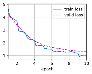
num_epochs, lr, wd = 10, 1e-4, 1e-4
lr_period, lr_decay = 2, 0.9
backbone, head = get_net()
head = train(backbone, head, train_iter, valid_iter, num_epochs, lr, wd,
             lr_period, lr_decay)
train loss 0.373, valid loss 1.281
99.1 examples/sec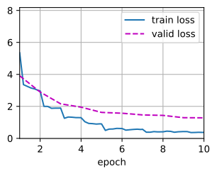
num_epochs, lr, wd = 10, 1e-4, 1e-4
lr_period, lr_decay = 2, 0.9
backbone, output_net = get_net()
output_net = train(backbone, output_net, train_iter, valid_iter, num_epochs,
                   lr, wd, lr_period, lr_decay)
train loss 4.282, valid loss 4.365
2032.5 examples/sec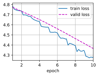
devices, num_epochs, lr, wd = d2l.try_all_gpus(), 10, 5e-3, 1e-4
lr_period, lr_decay, net = 2, 0.9, get_net(devices)
net.hybridize()
train(net, train_iter, valid_iter, num_epochs, lr, wd, devices, lr_period,
      lr_decay)
train loss 0.899, valid loss 0.879
376.9 examples/sec on [gpu(0)]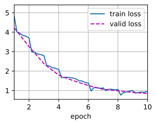
20.14.7 Classifying the Testing Set and Submitting Results on Kaggle
Similar to the final step in Section 20.13, in the end all the labeled data (including the validation set) are used for training the model and classifying the testing set. We will use the trained custom output network for classification.
net = get_net(devices)
train(net, train_valid_iter, None, num_epochs, lr, wd, devices, lr_period,
      lr_decay)

preds = []
for data, label in test_iter:
    output = torch.nn.functional.softmax(net(data.to(devices[0])), dim=1)
    preds.extend(output.cpu().detach().numpy())
ids = sorted(os.listdir(
    os.path.join(data_dir, 'train_valid_test', 'test', 'unknown')))
with open('submission.csv', 'w') as f:
    f.write('id,' + ','.join(train_valid_ds.classes) + '\n')
    for i, output in zip(ids, preds):
        f.write(i.split('.')[0] + ',' + ','.join(
            [str(num) for num in output]) + '\n')
train loss 1.070
3018.6 examples/sec on [device(type='cuda', index=0)]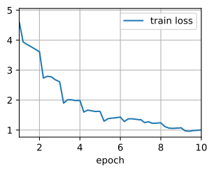
backbone, head = get_net()
head = train(backbone, head, train_valid_iter, None, num_epochs, lr, wd,
             lr_period, lr_decay)
preds = []
for data, label in test_iter:
    logits = head(backbone_features(backbone, data), training=False)
    output = tf.nn.softmax(logits, axis=-1)
    preds.extend(output.numpy())
# Get class names from the train_valid dataset directory
class_names = sorted(os.listdir(
    os.path.join(data_dir, 'train_valid_test', 'train_valid')))
ids = sorted(os.listdir(
    os.path.join(data_dir, 'train_valid_test', 'test', 'unknown')))
with open('submission.csv', 'w') as f:
    f.write('id,' + ','.join(class_names) + '\n')
    for i, output in zip(ids, preds):
        f.write(i.split('.')[0] + ',' + ','.join(
            [str(num) for num in output]) + '\n')
train loss 0.296
101.6 examples/sec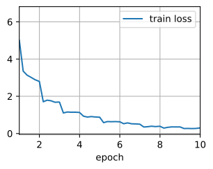
backbone, output_net = get_net()
output_net = train(backbone, output_net, train_valid_iter, None, num_epochs,
                   lr, wd, lr_period, lr_decay)

preds = []
for data, label in test_iter:
    feats = extract_features(backbone, data.numpy())
    logits = output_net(feats)
    output = jax.nn.softmax(logits, axis=-1)
    preds.extend(np.array(output))
# Get class names from the train_valid dataset directory
class_names = sorted(os.listdir(
    os.path.join(data_dir, 'train_valid_test', 'train_valid')))
ids = sorted(os.listdir(
    os.path.join(data_dir, 'train_valid_test', 'test', 'unknown')))
with open('submission.csv', 'w') as f:
    f.write('id,' + ','.join(class_names) + '\n')
    for i, output in zip(ids, preds):
        f.write(i.split('.')[0] + ',' + ','.join(
            [str(num) for num in output]) + '\n')
train loss 4.198
4580.3 examples/sec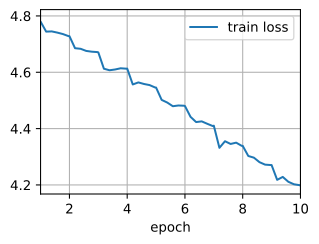
net = get_net(devices)
net.hybridize()
train(net, train_valid_iter, None, num_epochs, lr, wd, devices, lr_period,
      lr_decay)

preds = []
for data, label in test_iter:
    output_features = net.features(data.as_in_ctx(devices[0]))
    output = npx.softmax(net.output_new(output_features))
    preds.extend(output.asnumpy())
ids = sorted(os.listdir(
    os.path.join(data_dir, 'train_valid_test', 'test', 'unknown')))
with open('submission.csv', 'w') as f:
    f.write('id,' + ','.join(train_valid_ds.synsets) + '\n')
    for i, output in zip(ids, preds):
        f.write(i.split('.')[0] + ',' + ','.join(
            [str(num) for num in output]) + '\n')
train loss 0.830
408.4 examples/sec on [gpu(0)]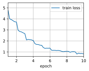
The above code will generate a submission.csv file to be submitted to Kaggle in the same way described in Section 4.7.
20.14.8 Summary
- Images in the ImageNet dataset are larger (with varying dimensions) than CIFAR-10 images. We may modify image augmentation operations for tasks on a different dataset.
- To classify a subset of the ImageNet dataset, we can leverage pre-trained models on the full ImageNet dataset to extract features and only train a custom small-scale output network. This will lead to less computational time and memory cost.
20.14.9 Exercises
- When using the full Kaggle competition dataset, what results can you achieve when you increase
batch_size(batch size) andnum_epochs(number of epochs) while setting some other hyperparameters aslr = 0.01,lr_period = 10, andlr_decay = 0.1? - Do you get better results if you use a deeper pretrained model? How do you tune hyperparameters? Can you further improve the results?