%matplotlib inline
from d2l import torch as d2l
import math
import torch
from torch import nn
from torch.nn import functional as F9.6 Adam
Momentum (Section 9.5) averages gradients over time but still uses the same learning rate for every coordinate. This can be inefficient when coordinates differ substantially in scale or curvature. This section develops adaptive per-coordinate learning rates through three related methods: AdaGrad scales every coordinate by the history of its own gradients, RMSProp makes that history forget, and Adam (Kingma and Ba 2015) adds momentum back in and corrects the startup bias. Adam-family methods became common defaults for transformer training, while tuned SGD with momentum remains competitive in several computer-vision settings.
The second half of the section examines when Adam improves on momentum. We introduce the testbed that the rest of the chapter trains on, a tiny transformer language model, and compare tuned Adam with tuned SGD with momentum on this model and on a convolutional network. The comparison isolates settings in which per-coordinate adaptation is most useful.
%matplotlib inline
from d2l import jax as d2l
from flax import nnx
import jax
from jax import numpy as jnp
import math
import optax
9.6.1 From AdaGrad to Adam
9.6.1.1 Per-Coordinate Learning Rates
Consider learning problems whose features occur with very different frequencies. This is the normal state of affairs in language: we will see the word learning far more often than the word preconditioning. The same imbalance appears in computational advertising and collaborative filtering, where most items interest only a few users. Parameters tied to rare features receive meaningful gradients only when those features occur. Under the decaying learning rate that stochastic convergence demands (Section 9.3), the parameters of frequent features approach their optima quickly while the rare ones are still waiting for evidence; by the time it arrives, the shared step size has decayed too far to use it. One clock cannot serve both populations.
AdaGrad (Duchi et al. 2011) gives every coordinate its own clock. Instead of decaying the step with wall-clock time \(t\), it decays each coordinate’s step with that coordinate’s own accumulated activity, measured by the running sum of its squared gradients:
\[ \mathbf{s}_t = \mathbf{s}_{t-1} + \mathbf{g}_t^2, \qquad \mathbf{x}_{t+1} = \mathbf{x}_t - \frac{\eta}{\sqrt{\mathbf{s}_t + \epsilon}} \odot \mathbf{g}_t, \tag{9.6.1}\]
with all operations elementwise, \(\mathbf{s}_0 = \mathbf{0}\), and a small \(\epsilon > 0\) guarding the division. A coordinate whose gradients have been large moves cautiously from now on; a coordinate that has barely been touched keeps a large step and can respond the moment its rare feature appears.
There is a second, deeper reading. For the ill-conditioned valley of Section 9.5, the ideal fix is to rescale each eigendirection by its curvature, which is a preconditioner. Computing curvature is out of the question at deep-learning scale, but when the coordinate axes roughly align with the eigendirections, the gradient’s own magnitude history is a usable proxy for the diagonal of the Hessian, and Equation 9.6.1 is exactly a diagonal preconditioner estimated from first-order information alone. Both readings can be made precise; the metric and regret derivations live in Section 26.2.2.
The following quadratic illustrates per-coordinate scaling \(f(\mathbf{x}) = 0.1 x_1^2 + 2 x_2^2\) from Section 9.5, with the same learning rate \(\eta = 0.4\) that plain gradient descent could only use timidly.
def adagrad_2d(x1, x2, s1, s2):
    eps = 1e-6
    g1, g2 = 0.2 * x1, 4 * x2
    s1 += g1 ** 2
    s2 += g2 ** 2
    x1 -= eta / math.sqrt(s1 + eps) * g1
    x2 -= eta / math.sqrt(s2 + eps) * g2
    return x1, x2, s1, s2

def f_2d(x1, x2):
    return 0.1 * x1 ** 2 + 2 * x2 ** 2

eta = 0.4
d2l.show_trace_2d(f_2d, d2l.train_2d(adagrad_2d))epoch 20, x1: -2.382563, x2: -0.158591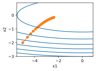
epoch 20, x1: -2.382563, x2: -0.158591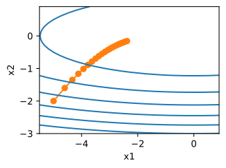
The trajectory is smooth: the steep \(x_2\) direction is scaled down automatically, so there is none of the oscillation that limited gradient descent. But the accumulation in \(\mathbf{s}_t\) also shows its cost within twenty steps: the effective learning rate keeps shrinking, and the iterate crawls long before it reaches the minimum. Because the scaling is adaptive, we can compensate with a learning rate that would have been unthinkable before, \(\eta = 2\):
eta = 2
d2l.show_trace_2d(f_2d, d2l.train_2d(adagrad_2d))epoch 20, x1: -0.002295, x2: -0.000000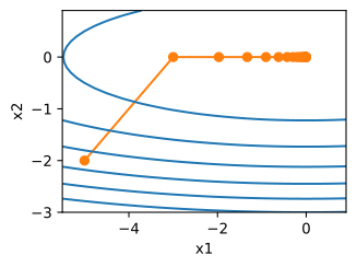
epoch 20, x1: -0.002295, x2: -0.000000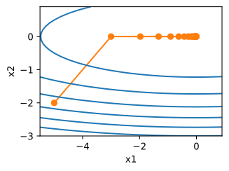
The from-scratch implementation for a real model keeps one accumulator per parameter. We train it on the airfoil dataset with the harness from Section 9.4, using a larger learning rate than SGD could tolerate there.
def init_adagrad_states(feature_dim):
    s_w = d2l.zeros((feature_dim, 1))
    s_b = d2l.zeros(1)
    return (s_w, s_b)

def adagrad(params, states, hyperparams):
    eps = 1e-6
    for p, s in zip(params, states):
        with torch.no_grad():
            s[:] += torch.square(p.grad)
            p[:] -= hyperparams['lr'] * p.grad / torch.sqrt(s + eps)
        p.grad.zero_()
def init_adagrad_states(feature_dim):
s_w = jnp.zeros((feature_dim, 1))
s_b = jnp.zeros(1)
return [s_w, s_b]
def adagrad(params, grads, states, hyperparams):
eps = 1e-6
for i, (p, s, g) in enumerate(zip(params, states, grads)):
s = s + jnp.square(g)
params[i] = p - hyperparams['lr'] * g / jnp.sqrt(s + eps)
states[i] = s
return params[0], params[1]data_iter, feature_dim = d2l.get_data_ch11(batch_size=10)
d2l.train_ch11(adagrad, init_adagrad_states(feature_dim),
{'lr': 0.1}, data_iter, feature_dim);loss: 0.243, 0.113 sec/epoch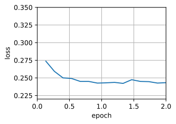
loss: 0.243, 1.447 sec/epoch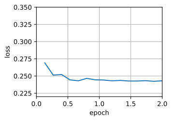
9.6.1.2 RMSProp: An Exponential Average
AdaGrad’s accumulator never forgets. Since \(\mathbf{s}_t\) grows without bound, roughly linearly under persistent gradient noise, the effective step decays like \(\mathcal{O}(t^{-1/2})\) whether or not the optimization is anywhere near done. This decay is appropriate for the convex settings that motivated AdaGrad, but can be too aggressive for a nonconvex objective that requires substantial movement late in training.
RMSProp (Tieleman and Hinton 2012) keeps the per-coordinate scaling and discards the lifetime memory, replacing the sum with an exponential moving average, the same leaky averaging that momentum applies to the gradient itself:
\[ \mathbf{v}_t = \beta_2\, \mathbf{v}_{t-1} + (1 - \beta_2)\, \mathbf{g}_t^2, \qquad \mathbf{x}_{t+1} = \mathbf{x}_t - \frac{\eta}{\sqrt{\mathbf{v}_t + \epsilon}} \odot \mathbf{g}_t. \tag{9.6.2}\]
The average \(\mathbf{v}_t\) now estimates the current squared-gradient scale rather than the lifetime total, over a window of about \(1/(1-\beta_2)\) steps, ten at the customary \(\beta_2 = 0.9\). The step size no longer decays by construction, and the learning rate \(\eta\) becomes a knob we control separately, to be scheduled on its own terms (Section 9.8). On the toy quadratic, RMSProp at \(\eta = 0.4\) makes steady progress where AdaGrad stalled:
def rmsprop_2d(x1, x2, v1, v2):
    g1, g2, eps = 0.2 * x1, 4 * x2, 1e-6
    v1 = beta2 * v1 + (1 - beta2) * g1 ** 2
    v2 = beta2 * v2 + (1 - beta2) * g2 ** 2
    x1 -= eta / math.sqrt(v1 + eps) * g1
    x2 -= eta / math.sqrt(v2 + eps) * g2
    return x1, x2, v1, v2

eta, beta2 = 0.4, 0.9
d2l.show_trace_2d(f_2d, d2l.train_2d(rmsprop_2d))epoch 20, x1: -0.010599, x2: 0.000000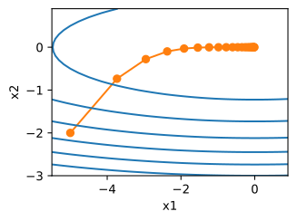
epoch 20, x1: -0.010599, x2: 0.000000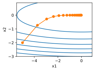
The implementation changes one line relative to AdaGrad, and the state layout is identical, so we reuse init_adagrad_states.
def rmsprop(params, states, hyperparams):
    beta2, eps = hyperparams['beta2'], 1e-6
    for p, v in zip(params, states):
        with torch.no_grad():
            v[:] = beta2 * v + (1 - beta2) * torch.square(p.grad)
            p[:] -= hyperparams['lr'] * p.grad / torch.sqrt(v + eps)
        p.grad.zero_()
def rmsprop(params, grads, states, hyperparams):
beta2, eps = hyperparams['beta2'], 1e-6
for i, (p, v, g) in enumerate(zip(params, states, grads)):
v = beta2 * v + (1 - beta2) * jnp.square(g)
params[i] = p - hyperparams['lr'] * g / jnp.sqrt(v + eps)
states[i] = v
return params[0], params[1]d2l.train_ch11(rmsprop, init_adagrad_states(feature_dim),
{'lr': 0.01, 'beta2': 0.9}, data_iter, feature_dim);loss: 0.246, 0.090 sec/epoch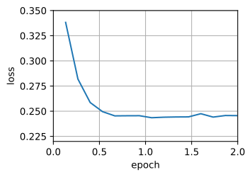
loss: 0.244, 0.449 sec/epoch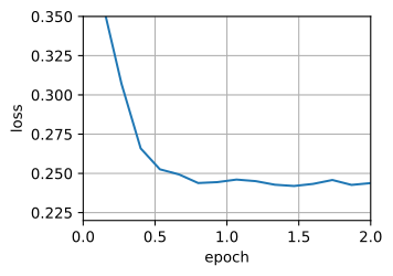
9.6.1.3 Adam: Both Moments, Debiased
Adam assembles the pieces. It applies the same exponential averaging to the gradient itself, giving a momentum estimate \(\mathbf{m}_t\) (the averaged form of the heavy-ball buffer from Section 9.5), keeps RMSProp’s second-moment estimate \(\mathbf{v}_t\), and corrects both for their zero initialization:
\[ \begin{aligned} \mathbf{m}_t &= \beta_1\, \mathbf{m}_{t-1} + (1 - \beta_1)\, \mathbf{g}_t, \qquad & \hat{\mathbf{m}}_t &= \mathbf{m}_t / (1 - \beta_1^t), \\ \mathbf{v}_t &= \beta_2\, \mathbf{v}_{t-1} + (1 - \beta_2)\, \mathbf{g}_t^2, \qquad & \hat{\mathbf{v}}_t &= \mathbf{v}_t / (1 - \beta_2^t), \end{aligned} \tag{9.6.3}\]
\[ \mathbf{x}_{t+1} = \mathbf{x}_t - \eta\, \frac{\hat{\mathbf{m}}_t}{\sqrt{\hat{\mathbf{v}}_t} + \epsilon}. \tag{9.6.4}\]
The defaults are \(\beta_1 = 0.9\) and \(\beta_2 = 0.999\): the direction estimate averages over roughly ten steps, while the scale estimate averages over roughly a thousand, a hundred times longer than RMSProp’s window.
The corrections in Equation 9.6.3 deserve a sentence of respect, because they are exact rather than heuristic. Starting from \(\mathbf{v}_0 = \mathbf{0}\), the average \(\mathbf{v}_t\) is a weighted sum whose weights total \(1 - \beta_2^t\), not \(1\); if the squared-gradient scale is locally stationary, then \(\mathbb{E}[\mathbf{v}_t]\) carries exactly the fraction \(1 - \beta_2^t\) of the true scale, and dividing by that fraction cancels the deficit identically at every \(t\). The transient being cancelled is not small: at \(\beta_2 = 0.999\), after ten steps \(\mathbf{v}_t\) holds about \(1\%\) of its stationary value, so uncorrected Adam would take its most aggressive steps precisely when its scale estimate is built from the fewest samples. Section 26.2.2 derives this transient behavior.
One more difference from Equation 9.6.2: Adam adds \(\epsilon\) outside the square root. At this demo’s scales, where \(\sqrt{\hat{\mathbf{v}}_t}\) is of order one, the placement matters little. It decides the update where \(\sqrt{\hat{\mathbf{v}}_t}\) is small, as with sparse gradients or mixed precision, and the \(\eta/\epsilon\) step ceiling we meet at the end of the section depends on it. We use \(\epsilon = 10^{-6}\) in the code below, while framework implementations default to \(10^{-8}\).
The implementation carries two buffers per parameter and a step counter for the bias correction, which we keep in the hyperparams dictionary.
def init_adam_states(feature_dim):
    m_w, m_b = d2l.zeros((feature_dim, 1)), d2l.zeros(1)
    v_w, v_b = d2l.zeros((feature_dim, 1)), d2l.zeros(1)
    return ((m_w, v_w), (m_b, v_b))

def adam(params, states, hyperparams):
    beta1, beta2, eps = 0.9, 0.999, 1e-6
    for p, (m, v) in zip(params, states):
        with torch.no_grad():
            m[:] = beta1 * m + (1 - beta1) * p.grad
            v[:] = beta2 * v + (1 - beta2) * torch.square(p.grad)
            m_hat = m / (1 - beta1 ** hyperparams['t'])
            v_hat = v / (1 - beta2 ** hyperparams['t'])
            p[:] -= hyperparams['lr'] * m_hat / (torch.sqrt(v_hat) + eps)
        p.grad.zero_()
    hyperparams['t'] += 1
def init_adam_states(feature_dim):
m_w, m_b = jnp.zeros((feature_dim, 1)), jnp.zeros(1)
v_w, v_b = jnp.zeros((feature_dim, 1)), jnp.zeros(1)
return [(m_w, v_w), (m_b, v_b)]
def adam(params, grads, states, hyperparams):
beta1, beta2, eps = 0.9, 0.999, 1e-6
for i, (p, (m, v), g) in enumerate(zip(params, states, grads)):
m = beta1 * m + (1 - beta1) * g
v = beta2 * v + (1 - beta2) * jnp.square(g)
m_hat = m / (1 - beta1 ** hyperparams['t'])
v_hat = v / (1 - beta2 ** hyperparams['t'])
params[i] = p - hyperparams['lr'] * m_hat / (jnp.sqrt(v_hat) + eps)
states[i] = (m, v)
hyperparams['t'] += 1
return params[0], params[1]d2l.train_ch11(adam, init_adam_states(feature_dim),
{'lr': 0.01, 't': 1}, data_iter, feature_dim);loss: 0.243, 0.100 sec/epoch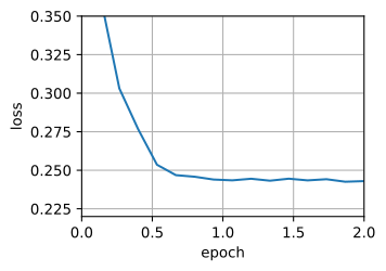
loss: 0.244, 0.717 sec/epoch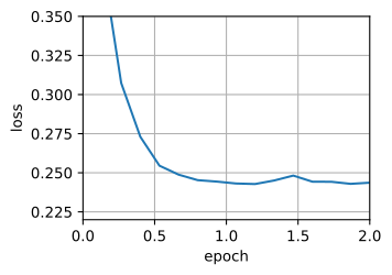
In practice one calls the framework implementation, which follows Equation 9.6.3 and Equation 9.6.4 up to small conventions that differ by framework and version: where \(\epsilon\) sits relative to the square root, optional flags such as AMSGrad, and the precise bias-correction bookkeeping. None of this usually matters at default settings.
trainer = torch.optim.Adam
d2l.train_concise_ch11(trainer, {'lr': 0.01}, data_iter)
loss: 0.242, 0.099 sec/epoch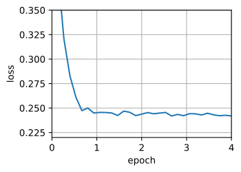
trainer = optax.adam
d2l.train_concise_ch11(trainer, {'learning_rate': 0.01}, data_iter)
loss: 0.245, 0.400 sec/epoch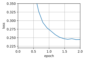
Note what the two extra buffers cost: Adam stores two floats of state for every parameter of the model, tripling the memory a parameter occupies before activations and gradients are counted. At the scale of this chapter’s models the cost is invisible; at the scale of language models it dictates hardware budgets, and we return to the accounting in the next section.
9.6.2 A Tiny Language Model
On the airfoil problem every optimizer in this chapter looks fine, and on small image models the differences stay small. Language models provide a setting in which modern optimizers differ more substantially. We therefore build a small language model that exhibits these differences and use it as the chapter’s testbed.
The reader has trained language models on exactly this data before: The Time Machine, tokenized and batched as in Section 8.2, with quality measured in perplexity as in Section 8.3. Only the architecture is new. TinyLM is a decoder-only transformer, the architecture of Chapter 11, and we are deliberately using it two chapters early: the optimization discussion does not require the details of attention. Here the model is a differentiable function with several parameter groups, and the optimizer acts on their gradients rather than on the attention mechanism directly.
data = d2l.TimeMachine(batch_size=64, num_steps=64, tokenization='char',
                       num_train=100000)
The model: learned token and position embeddings, two pre-norm transformer blocks (attention plus a two-layer MLP, each behind a LayerNorm, each with a residual connection), and a linear head that predicts the next character. The attention primitive is a single library call.
class TinyLM(nn.Module):
    """A small decoder-only transformer language model."""
    def __init__(self, vocab_size, d_model=128, num_heads=2, num_blks=2,
                 max_len=64):
        super().__init__()
        self.num_heads = num_heads
        self.token_emb = nn.Embedding(vocab_size, d_model)
        self.pos_emb = nn.Embedding(max_len, d_model)
        self.blks = nn.ModuleList([nn.ModuleDict(dict(
            norm1=nn.LayerNorm(d_model),
            qkv=nn.Linear(d_model, 3 * d_model),
            proj=nn.Linear(d_model, d_model),
            norm2=nn.LayerNorm(d_model),
            mlp=nn.Sequential(nn.Linear(d_model, 4 * d_model), nn.GELU(),
                              nn.Linear(4 * d_model, d_model))))
            for _ in range(num_blks)])
        self.norm = nn.LayerNorm(d_model)
        self.head = nn.Linear(d_model, vocab_size)

    def attention(self, blk, X):
        B, T, D = X.shape
        q, k, v = blk['qkv'](X).chunk(3, dim=-1)
        q, k, v = (u.reshape(B, T, self.num_heads, -1).transpose(1, 2)
                   for u in (q, k, v))
        Y = F.scaled_dot_product_attention(q, k, v, is_causal=True)
        return blk['proj'](Y.transpose(1, 2).reshape(B, T, D))

    def forward(self, X):
        H = self.token_emb(X) + self.pos_emb(torch.arange(X.shape[1],
                                                          device=X.device))
        for blk in self.blks:
            H = H + self.attention(blk, blk['norm1'](H))
            H = H + blk['mlp'](blk['norm2'](H))
        return self.head(self.norm(H))
class TinyLM(nnx.Module):
"""A small decoder-only transformer language model."""
def __init__(self, vocab_size, d_model=128, num_heads=2, num_blks=2,
max_len=64, rngs=None):
rngs = nnx.Rngs(0) if rngs is None else rngs
self.num_heads = num_heads
self.token_emb = nnx.Embed(vocab_size, d_model, rngs=rngs)
self.pos_emb = nnx.Embed(max_len, d_model, rngs=rngs)
self.blks = nnx.List([nnx.Dict(
norm1=nnx.LayerNorm(d_model, rngs=rngs),
qkv=nnx.Linear(d_model, 3 * d_model, rngs=rngs),
proj=nnx.Linear(d_model, d_model, rngs=rngs),
norm2=nnx.LayerNorm(d_model, rngs=rngs),
mlp1=nnx.Linear(d_model, 4 * d_model, rngs=rngs),
mlp2=nnx.Linear(4 * d_model, d_model, rngs=rngs))
for _ in range(num_blks)])
self.norm = nnx.LayerNorm(d_model, rngs=rngs)
self.head = nnx.Linear(d_model, vocab_size, rngs=rngs)
def attention(self, blk, X):
B, T, D = X.shape
q, k, v = jnp.split(blk['qkv'](X), 3, axis=-1)
q, k, v = (u.reshape(B, T, self.num_heads, -1) for u in (q, k, v))
Y = jax.nn.dot_product_attention(q, k, v, is_causal=True)
return blk['proj'](Y.reshape(B, T, D))
def __call__(self, X):
H = self.token_emb(X) + self.pos_emb(jnp.arange(X.shape[1]))
for blk in self.blks:
H = H + self.attention(blk, blk['norm1'](H))
H = H + blk['mlp2'](jax.nn.gelu(blk['mlp1'](blk['norm2'](H))))
return self.head(self.norm(H))Before training, we group the parameters into three populations: embeddings, whose rows receive gradients only when their token occurs, the sparse features that motivated AdaGrad; two-dimensional matrices, which hold nearly all of the parameters; and one-dimensional vectors, the LayerNorm scales and biases. Later sections treat these populations differently, deciding which ones to weight-decay and which ones a matrix preconditioner should own, so this table is worth a moment of study.
model = TinyLM(vocab_size=len(data.vocab))
kinds = {'embeddings': 0, 'matrices': 0, 'vectors': 0}
print(f'{"parameter":<22} {"shape":<14} {"count":>7}')
for name, p in model.named_parameters():
    kind = ('embeddings' if 'emb' in name else
            'matrices' if p.ndim == 2 else 'vectors')
    kinds[kind] += p.numel()
    print(f'{name:<22} {str(tuple(p.shape)):<14} {p.numel():>7}')
for kind, count in kinds.items():
    print(f'{kind:>37} {count:>7}')
print(f'{"total":>37} {sum(kinds.values()):>7}')
parameter shape count
token_emb.weight (28, 128) 3584
pos_emb.weight (64, 128) 8192
blks.0.norm1.weight (128,) 128
blks.0.norm1.bias (128,) 128
blks.0.qkv.weight (384, 128) 49152
blks.0.qkv.bias (384,) 384
blks.0.proj.weight (128, 128) 16384
blks.0.proj.bias (128,) 128
blks.0.norm2.weight (128,) 128
blks.0.norm2.bias (128,) 128
blks.0.mlp.0.weight (512, 128) 65536
blks.0.mlp.0.bias (512,) 512
blks.0.mlp.2.weight (128, 512) 65536
blks.0.mlp.2.bias (128,) 128
blks.1.norm1.weight (128,) 128
blks.1.norm1.bias (128,) 128
blks.1.qkv.weight (384, 128) 49152
blks.1.qkv.bias (384,) 384
blks.1.proj.weight (128, 128) 16384
blks.1.proj.bias (128,) 128
blks.1.norm2.weight (128,) 128
blks.1.norm2.bias (128,) 128
blks.1.mlp.0.weight (512, 128) 65536
blks.1.mlp.0.bias (512,) 512
blks.1.mlp.2.weight (128, 512) 65536
blks.1.mlp.2.bias (128,) 128
norm.weight (128,) 128
norm.bias (128,) 128
head.weight (28, 128) 3584
head.bias (28,) 28
embeddings 11776
matrices 396800
vectors 3612
total 412188model = TinyLM(vocab_size=len(data.vocab))
kinds = {'embeddings': 0, 'matrices': 0, 'vectors': 0}
print(f'{"parameter":<22} {"shape":<14} {"count":>7}')
for path, p in nnx.to_flat_state(nnx.state(model, nnx.Param)):
name = '.'.join(str(k) for k in path)
kind = ('embeddings' if 'emb' in name else
'matrices' if p.ndim == 2 else 'vectors')
kinds[kind] += p.size
print(f'{name:<22} {str(tuple(p.shape)):<14} {p.size:>7}')
for kind, count in kinds.items():
print(f'{kind:>37} {count:>7}')
print(f'{"total":>37} {sum(kinds.values()):>7}')parameter shape count
blks.0.mlp1.bias (512,) 512
blks.0.mlp1.kernel (128, 512) 65536
blks.0.mlp2.bias (128,) 128
blks.0.mlp2.kernel (512, 128) 65536
blks.0.norm1.bias (128,) 128
blks.0.norm1.scale (128,) 128
blks.0.norm2.bias (128,) 128
blks.0.norm2.scale (128,) 128
blks.0.proj.bias (128,) 128
blks.0.proj.kernel (128, 128) 16384
blks.0.qkv.bias (384,) 384
blks.0.qkv.kernel (128, 384) 49152
blks.1.mlp1.bias (512,) 512
blks.1.mlp1.kernel (128, 512) 65536
blks.1.mlp2.bias (128,) 128
blks.1.mlp2.kernel (512, 128) 65536
blks.1.norm1.bias (128,) 128
blks.1.norm1.scale (128,) 128
blks.1.norm2.bias (128,) 128
blks.1.norm2.scale (128,) 128
blks.1.proj.bias (128,) 128
blks.1.proj.kernel (128, 128) 16384
blks.1.qkv.bias (384,) 384
blks.1.qkv.kernel (128, 384) 49152
head.bias (28,) 28
head.kernel (128, 28) 3584
norm.bias (128,) 128
norm.scale (128,) 128
pos_emb.embedding (64, 128) 8192
token_emb.embedding (28, 128) 3584
embeddings 11776
matrices 396800
vectors 3612
total 412188About 0.4 million parameters, 96% of them in the matrices. Training is a plain step-counted loop: stream minibatches, compute the mean cross-entropy of the next-character prediction, step the optimizer, record the loss. We save it for reuse by the rest of the chapter.
def train_lm(model, data, optimizer, num_steps):
    """Train a model on next-token prediction for a fixed number of steps."""
    device = d2l.try_gpu()
    model.to(device)
    losses, step = [], 0
    while step < num_steps:
        for X, Y in data.train_dataloader():
            X, Y = X.to(device), Y.to(device)
            logits = model(X)
            loss = F.cross_entropy(logits.reshape(-1, logits.shape[-1]),
                                   Y.reshape(-1))
            optimizer.zero_grad()
            loss.backward()
            optimizer.step()
            losses.append(loss.item())
            step += 1
            if step >= num_steps:
                return losses
def train_lm(model, data, optimizer, num_steps):
"""Train a model on next-token prediction for a fixed number of steps."""
@nnx.jit
def step_fn(model, optimizer, X, Y):
def loss_fn(model):
logits = model(X)
return optax.softmax_cross_entropy_with_integer_labels(
logits.reshape(-1, logits.shape[-1]), Y.reshape(-1)).mean()
loss, grads = nnx.value_and_grad(loss_fn)(model)
optimizer.update(model, grads)
return loss
losses, step = [], 0
while step < num_steps:
for X, Y in data.train_dataloader():
loss = step_fn(model, optimizer, jnp.asarray(X), jnp.asarray(Y))
losses.append(float(loss))
step += 1
if step >= num_steps:
return lossesTwo small helpers finish the toolkit: the final loss averaged over the last hundred steps (with divergence mapped to infinity, which the experiments below will need), and a smoothed curve for plotting.
def final_loss(losses, k=100):
    v = sum(losses[-k:]) / k
    return v if math.isfinite(v) else float('inf')

def smooth(losses, k=25):
    return [sum(losses[i:i + k]) / k
            for i in range(0, len(losses) - k + 1, k)]
A first run with Adam at \(\eta = 0.003\), for 2,000 steps, about twenty seconds on one GPU:
model = TinyLM(len(data.vocab))
optimizer = torch.optim.Adam(model.parameters(), lr=0.003)
losses = train_lm(model, data, optimizer, num_steps=2000)
d2l.plot(list(range(0, 2000, 25)), [smooth(losses)],
         'step', 'training loss')
print(f'perplexity per character: {math.exp(final_loss(losses)):.2f}')
perplexity per character: 2.51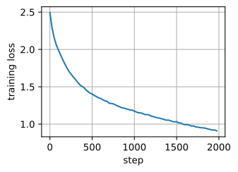
model = TinyLM(len(data.vocab))
optimizer = nnx.Optimizer(model, optax.adam(0.003), wrt=nnx.Param)
losses = train_lm(model, data, optimizer, num_steps=2000)
d2l.plot(list(range(0, 2000, 25)), [smooth(losses)],
         'step', 'training loss')
print(f'perplexity per character: {math.exp(final_loss(losses)):.2f}')
perplexity per character: 2.76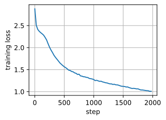
The model reaches a per-character perplexity below 3, against a uniform baseline of about 28 (the vocabulary size): it has learned a good deal of English spelling in those twenty seconds. A matched comparison can determine how much of this optimization speed depends on Adam.
9.6.3 Where Adam Wins
Practitioners reach for Adam on transformers because SGD, however tuned, does not keep up. On convolutional networks that folk wisdom is far weaker; SGD with momentum was the standard for a decade of vision. Rather than repeat the folklore, we run the comparison.
The protocol matters more than the contestants, because “optimizer A beats optimizer B” claims are notoriously sensitive to tuning effort (Schmidt et al. 2021). Ours is symmetric and small: both optimizers train the same model from the same initialization for the same 2,000 steps at a constant learning rate, with no schedule, clipping, or weight decay. Each gets a four-point learning-rate grid spaced by factors of about three, and the run with the best final training loss represents its family. Training loss is the relevant metric here: the question is which method optimizes faster, not who generalizes better.
9.6.3.1 Comparison on the Language Model
def run_lm(make_optimizer, lrs, num_steps=2000):
    curves = {}
    for lr in lrs:
        torch.manual_seed(0)
        model = TinyLM(len(data.vocab))
        curves[lr] = train_lm(model, data, make_optimizer(model, lr),
                              num_steps)
        print(f'lr {lr:g}: final loss {final_loss(curves[lr]):.3f}')
    return curves

sgd_lm = run_lm(lambda model, lr: torch.optim.SGD(model.parameters(), lr,
                                                  momentum=0.9),
                lrs=[0.03, 0.1, 0.3, 1.0])
lr 0.03: final loss 1.971
lr 0.1: final loss 1.418
lr 0.3: final loss 1.073
lr 1: final loss infdef run_lm(make_tx, lrs, num_steps=2000):
curves = {}
for lr in lrs:
model = TinyLM(len(data.vocab), rngs=nnx.Rngs(0))
optimizer = nnx.Optimizer(model, make_tx(lr), wrt=nnx.Param)
curves[lr] = train_lm(model, data, optimizer, num_steps)
print(f'lr {lr:g}: final loss {final_loss(curves[lr]):.3f}')
return curves
sgd_lm = run_lm(lambda lr: optax.sgd(lr, momentum=0.9),
lrs=[0.03, 0.1, 0.3, 1.0])lr 0.03: final loss 1.343
lr 0.1: final loss 1.206
lr 0.3: final loss inf
lr 1: final loss infadam_lm = run_lm(lambda model, lr: torch.optim.Adam(model.parameters(), lr),
lrs=[3e-4, 1e-3, 3e-3, 1e-2])lr 0.0003: final loss 1.506
lr 0.001: final loss 1.157
lr 0.003: final loss 0.912
lr 0.01: final loss 0.975adam_lm = run_lm(optax.adam, lrs=[3e-4, 1e-3, 3e-3, 1e-2])lr 0.0003: final loss 1.310
lr 0.001: final loss 0.994
lr 0.003: final loss 1.040
lr 0.01: final loss 2.263On this grid, SGD’s best learning rate sits directly below a divergent one: moving one grid point higher produces a NaN loss. Adam’s optimum is interior, with stable neighboring rates on both sides. This experiment establishes the difference for this model and grid; it does not by itself identify gradient tails as the cause or characterize all transformers. We compare the best rate found for each method:
best_sgd = min(sgd_lm, key=lambda lr: final_loss(sgd_lm[lr]))
best_adam = min(adam_lm, key=lambda lr: final_loss(adam_lm[lr]))
d2l.plot(list(range(0, 2000, 25)),
         [smooth(sgd_lm[best_sgd]), smooth(adam_lm[best_adam])],
         'step', 'training loss',
         legend=[f'SGD + momentum, lr {best_sgd:g}',
                 f'Adam, lr {best_adam:g}'])
print(f'final perplexity: SGD {math.exp(final_loss(sgd_lm[best_sgd])):.2f}, '
f'Adam {math.exp(final_loss(adam_lm[best_adam])):.2f}')final perplexity: SGD 2.92, Adam 2.49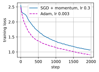
final perplexity: SGD 3.34, Adam 2.70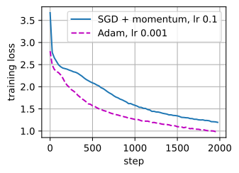
Tuned Adam beats tuned SGD (“tuned” here and below meaning the best of the coarse four-point grid) by a wide margin, roughly 20% in final training loss in our runs, and the gap is not a transient: Adam’s curve is below SGD’s at every point after the first few dozen steps and is still opening at the end. No rate in our grid rescued SGD: the sweep found its best, and the next one diverged. On this problem, per-coordinate scaling is worth more than any amount of step-size tuning.
9.6.3.2 Comparison on a CNN
We apply the same protocol to an image classifier: a compact convolutional network on Fashion-MNIST, defined in a few lines. Note that train_lm never asked its model to be a language model; it streams minibatches and computes cross-entropy, so the same harness trains the CNN unchanged.
fashion = d2l.FashionMNIST(batch_size=256)

def make_cnn():
    return nn.Sequential(
        nn.LazyConv2d(32, kernel_size=3, padding=1), nn.ReLU(),
        nn.MaxPool2d(2),
        nn.LazyConv2d(64, kernel_size=3, padding=1), nn.ReLU(),
        nn.MaxPool2d(2),
        nn.Flatten(), nn.LazyLinear(128), nn.ReLU(), nn.LazyLinear(10))

def test_accuracy(model, data):
    device = d2l.try_gpu()
    model.eval()
    correct = total = 0
    with torch.no_grad():
        for X, y in data.val_dataloader():
            X, y = X.to(device), y.to(device)
            correct += float((model(X).argmax(axis=1) == y).sum())
            total += y.numel()
    return correct / total
fashion = d2l.FashionMNIST(batch_size=256)
class FashionCNN(nnx.Module):
def __init__(self, rngs=None):
rngs = nnx.Rngs(0) if rngs is None else rngs
self.conv1 = nnx.Conv(1, 32, kernel_size=(3, 3), rngs=rngs)
self.conv2 = nnx.Conv(32, 64, kernel_size=(3, 3), rngs=rngs)
self.fc1 = nnx.Linear(64 * 7 * 7, 128, rngs=rngs)
self.fc2 = nnx.Linear(128, 10, rngs=rngs)
def __call__(self, X):
X = nnx.max_pool(nnx.relu(self.conv1(X)), window_shape=(2, 2),
strides=(2, 2))
X = nnx.max_pool(nnx.relu(self.conv2(X)), window_shape=(2, 2),
strides=(2, 2))
X = X.reshape(X.shape[0], -1)
return self.fc2(nnx.relu(self.fc1(X)))
def test_accuracy(model, data):
correct = total = 0
for X, y in data.val_dataloader():
pred = model(jnp.asarray(X)).argmax(axis=1)
correct += float((pred == jnp.asarray(y)).sum())
total += y.shape[0]
return correct / totaldef run_cnn(make_optimizer, lrs, num_steps=2000):
curves, accs = {}, {}
for lr in lrs:
torch.manual_seed(0)
model = make_cnn()
curves[lr] = train_lm(model, fashion, make_optimizer(model, lr),
num_steps)
accs[lr] = test_accuracy(model, fashion)
print(f'lr {lr:g}: final loss {final_loss(curves[lr]):.3f}, '
f'test accuracy {accs[lr]:.3f}')
return curves, accs
sgd_cnn, sgd_cnn_acc = run_cnn(
lambda model, lr: torch.optim.SGD(model.parameters(), lr, momentum=0.9),
lrs=[0.01, 0.03, 0.1, 0.3])lr 0.01: final loss 0.276, test accuracy 0.888
lr 0.03: final loss 0.200, test accuracy 0.900
lr 0.1: final loss 0.146, test accuracy 0.904
lr 0.3: final loss 2.305, test accuracy 0.100def run_cnn(make_tx, lrs, num_steps=2000):
curves, accs = {}, {}
for lr in lrs:
model = FashionCNN(rngs=nnx.Rngs(0))
optimizer = nnx.Optimizer(model, make_tx(lr), wrt=nnx.Param)
curves[lr] = train_lm(model, fashion, optimizer, num_steps)
accs[lr] = test_accuracy(model, fashion)
print(f'lr {lr:g}: final loss {final_loss(curves[lr]):.3f}, '
f'test accuracy {accs[lr]:.3f}')
return curves, accs
sgd_cnn, sgd_cnn_acc = run_cnn(lambda lr: optax.sgd(lr, momentum=0.9),
lrs=[0.01, 0.03, 0.1, 0.3])lr 0.01: final loss 0.243, test accuracy 0.899
lr 0.03: final loss 0.185, test accuracy 0.902
lr 0.1: final loss 0.132, test accuracy 0.919
lr 0.3: final loss 0.232, test accuracy 0.885adam_cnn, adam_cnn_acc = run_cnn(
lambda model, lr: torch.optim.Adam(model.parameters(), lr),
lrs=[3e-4, 1e-3, 3e-3, 1e-2])lr 0.0003: final loss 0.282, test accuracy 0.880
lr 0.001: final loss 0.185, test accuracy 0.902
lr 0.003: final loss 0.113, test accuracy 0.919
lr 0.01: final loss 0.152, test accuracy 0.897adam_cnn, adam_cnn_acc = run_cnn(optax.adam, lrs=[3e-4, 1e-3, 3e-3, 1e-2])lr 0.0003: final loss 0.241, test accuracy 0.898
lr 0.001: final loss 0.154, test accuracy 0.913
lr 0.003: final loss 0.091, test accuracy 0.920
lr 0.01: final loss 0.144, test accuracy 0.907best_sgd = min(sgd_cnn, key=lambda lr: final_loss(sgd_cnn[lr]))
best_adam = min(adam_cnn, key=lambda lr: final_loss(adam_cnn[lr]))
d2l.plot(list(range(0, 2000, 25)),
[smooth(sgd_cnn[best_sgd]), smooth(adam_cnn[best_adam])],
'step', 'training loss',
legend=[f'SGD + momentum, lr {best_sgd:g}',
f'Adam, lr {best_adam:g}'])
print(f'test accuracy: SGD {sgd_cnn_acc[best_sgd]:.3f}, '
f'Adam {adam_cnn_acc[best_adam]:.3f}')test accuracy: SGD 0.904, Adam 0.919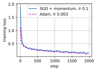
test accuracy: SGD 0.919, Adam 0.920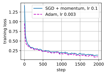
The CNN produces a different comparison. Both tuned optimizers drive the training loss into the same low regime along closely tracking curves, and their test accuracies land within a point or two of each other, around 90–92%; whatever residual edge remains is small and varies from run to run. Nothing here resembles the language-model gap: on this problem SGD is a competitive choice, which is why it carried computer vision for a decade. The interesting question is why the same two optimizers behave so differently on the two tasks.
9.6.3.3 Why the Gap Lives Where It Does
This is current research rather than settled textbook material, but its outline is clear, and all of its threads run through the parameter census.
First, the gap is not about minibatch noise. Kunstner et al. (2023) showed that it persists in full-batch training, where there is no noise to manage, and that Adam’s advantage tracks that of sign descent, the method that keeps only the sign of each gradient coordinate. The connection is visible in Equation 9.6.4: switch off both averages (\(\beta_1 = \beta_2 = 0\)) and the update becomes \(\eta\, \mathbf{g}_t / (|\mathbf{g}_t| + \epsilon)\), which is \(\eta\, \mathrm{sign}(\mathbf{g}_t)\). Adam is a smoothed sign method: what it mainly does on these problems is equalize the step across coordinates whose gradients differ enormously in magnitude.
Second, the disparities being equalized are real and structural. Language data is heavy-tailed: most tokens are rare, so the embedding rows and output columns that serve them see small, infrequent gradients, while frequent tokens see large, constant ones. Kunstner et al. (2024) showed that gradient descent stalls on the loss of the rare classes while Adam keeps making progress on all of them, and that the effect reproduces even in linear models with imbalanced classes. Third, the heterogeneity is architectural as well as lexical: across the blocks of a transformer, embedding, attention, and MLP parameters have curvature spectra so different that no single learning rate suits them all, whereas the blocks of a CNN look far more alike (Zhang et al. 2024). A per-coordinate method supplies every block its own effective step; a global method must use a rate small enough for the stiffest block, slowing updates elsewhere. The parameter groups provide a coarse version of this distinction: three populations with different geometry and different update statistics, all sharing one \(\eta\) under SGD.
None of these accounts is final, and they are not mutually exclusive. The character-level vocabulary here has no starved rare tokens: its frequencies are skewed, but unlike the rare words of a word-level vocabulary, even the rarest character recurs thousands of times over the run. The architectural heterogeneity alone still sustains a wide gap. What is settled is the practice: on transformers, use the method that scales per coordinate.
9.6.4 When the Variance Estimate Misbehaves
Adam’s preconditioner \(\hat{\mathbf{v}}_t\) is an estimate built from a single noisy gradient stream, and errors in this estimate can produce very large updates. When gradients are sparse or heavy-tailed, the exponential average forgets between informative events: a coordinate’s \(\hat{\mathbf{v}}\) decays toward zero during a sequence of small gradients, and the rare large gradient then arrives with an enormous effective step. Reddi et al. (2018) turned this into a theorem, exhibiting convex problems on which Adam converges to the worst point. Section 26.2.2 works through their construction, along with the one-line fix that keeps a running maximum of \(\hat{\mathbf{v}}_t\) (AMSGrad). A related repair, Yogi (Zaheer et al. 2018), controls how fast \(\mathbf{v}_t\) can shrink by making the update additive with a sign-controlled direction. Both are implemented in the exercises; neither displaced Adam in practice, but the failure mode they address is worth recognizing when a training run inexplicably blows up on rare inputs.
This is also what \(\epsilon\) is really for. Nominally a guard against division by zero, it is in fact a floor on the denominator of Equation 9.6.4, and therefore a ceiling of \(\eta/\epsilon\) on any coordinate’s effective step. A small \(\epsilon\) says “trust the variance estimate, even a tiny one”; a large \(\epsilon\) says “do not”, and in the limit of large \(\epsilon\) Adam degrades gracefully into SGD with momentum (Equation 9.5.2 with \(\beta = \beta_1\)) at learning rate \((1 - \beta_1)\eta/\epsilon\). Between the extremes lies a real tuning knob: values as large as \(10^{-4}\) or even \(10^{-2}\) are sometimes used where second-moment estimates are unreliable. The exercise below maps the interpolation.
9.6.5 Summary
Adam is three stacked estimates: AdaGrad’s insight that each coordinate should be scaled by its own gradient history, RMSProp’s correction that the history must forget (an exponential average with window \(1/(1-\beta_2)\)), and a momentum average of the gradient itself, with both averages debiased exactly against their zero initialization. The result is a diagonal preconditioner estimated from first-order information, cheap enough to run at any scale, while requiring two extra state buffers per parameter.
The improvement is not uniform across model classes. At matched tuning on a small transformer language model, Adam beats SGD with momentum decisively, and no rate in our grid closed the gap; on a comparable CNN the two are close. The best current explanations point at heterogeneity that a single global learning rate cannot serve, across token frequencies and across architectural blocks. The variance estimate at Adam’s heart can also misbehave; \(\epsilon\), AMSGrad, and Yogi are the standard responses.
9.6.6 Exercises
- [code] Adam’s learning rate on the airfoil data. The from-scratch
adamtrains the linear model withd2l.train_ch11at \(\eta = 0.01\).- Sweep \(\eta \in \{10^{-3}, 10^{-2}, 10^{-1}, 1\}\) and report the final loss of each run. Copy the
sgdupdate function of Section 9.4 into this notebook, repeat the sweep with it on the samedata_iter, and compare how the final loss of each method changes as \(\eta\) grows past its best value. - Explain from Equation 9.6.4 why the size of an Adam step in a coordinate is typically about \(\eta\) once the moment estimates have stabilized, whatever the scale of the gradient, and why this makes the usable range of \(\eta\) differ from that of SGD.
- Sweep \(\eta \in \{10^{-3}, 10^{-2}, 10^{-1}, 1\}\) and report the final loss of each run. Copy the
- Bias correction by initialization. Instead of the zero initialization and the corrections in Equation 9.6.3, initialize \(\mathbf{m}_1 = \mathbf{g}_1\) and \(\mathbf{v}_1 = \mathbf{g}_1^2\) and use the uncorrected averages from then on.
- Show that the two schemes coincide at \(t = 1\) and derive the weights that each assigns to \(\mathbf{g}_1, \ldots, \mathbf{g}_t\) for \(t > 1\).
- What is lost relative to the exact correction, and for which range of \(t\) does the difference matter?
- [code] The second-moment window. Rerun
run_lmfor Adam at the best learning rate ofadam_lmwith \(\beta_2 \in \{0.9, 0.99, 0.999, 0.9999\}\). Which direction hurts more, forgetting too fast or too slowly? Relate your finding to the averaging window \(1/(1-\beta_2)\) and to the 2,000-step budget. - [code] The \(\epsilon\) ceiling. Sweep \(\epsilon \in \{10^{-8}, 10^{-6}, 10^{-4}, 10^{-2}, 1\}\) for Adam on
TinyLMat the best learning rate ofadam_lm. Explain the trend at both ends of the sweep with the \(\eta/\epsilon\) step ceiling of Section 9.6.4, and identify the \(\epsilon\) from which the run resembles SGD with momentum, as insgd_lm, at learning rate \((1 - \beta_1)\eta/\epsilon\). - [code] Two repairs of the variance estimate. Adam’s second-moment update can be written as \[\mathbf{v}_t = \mathbf{v}_{t-1} + (1 - \beta_2)(\mathbf{g}_t^2 - \mathbf{v}_{t-1}),\] which shrinks \(\mathbf{v}_t\) whenever \(\mathbf{g}_t^2 < \mathbf{v}_{t-1}\). Yogi (Zaheer et al. 2018) caps the shrinkage rate by replacing the increment with \[(1 - \beta_2)\, \mathbf{g}_t^2 \odot \mathrm{sgn}(\mathbf{g}_t^2 - \mathbf{v}_{t-1}). \tag{9.6.5}\] AMSGrad (Reddi et al. 2018) carries the running maximum \[\hat{\mathbf{v}}_t^{\max} = \max(\hat{\mathbf{v}}_{t-1}^{\max}, \hat{\mathbf{v}}_t) \tag{9.6.6}\] and uses it in place of \(\hat{\mathbf{v}}_t\) in Equation 9.6.4. Implement Yogi and AMSGrad as update functions for
d2l.train_ch11, followingadam, and compare both withadamon the airfoil data. - [code] Yogi on the Reddi construction. ● The function
onlineof Section 26.2.2 runs Adam and AMSGrad on the losses Equation 26.2.6, on which Adam converges to the worst point \(x = +1\). Add the Yogi update of problem 5 to it, run it at \(C = 4\), and report where its iterate ends. Explain the outcome from how far the \(v_t\) of Adam and of Yogi can fall during the two \(-1\) gradients of each period. - [code] Adadelta. Adadelta (Zeiler 2012) extends RMSProp with a second exponential average, of the squared updates, whose square root replaces \(\eta\), so that the method nominally has no learning rate. Implement it as an update function for
d2l.train_ch11, followingrmsprop, and compare the two on the airfoil data. Where does the scale of the very first update come from? - [code] Rotating the coordinates. Per-coordinate methods are axis-aligned. Rotating the valley
f_2dby \(45^\circ\) gives \[f(\mathbf{x}) = 0.05 (x_1 + x_2)^2 + (x_1 - x_2)^2, \tag{9.6.7}\] whose Hessian has the same eigenvalues as that off_2d, \(0.2\) and \(4\).- Adapt the gradients in
adagrad_2dandrmsprop_2dto the rotated valley, and write its gradient function for thegd_2dof Section 9.5. On both valleys, run AdaGrad at \(\eta = 0.4\) and \(\eta = 2\), RMSProp at \(\eta = 0.4\), and gradient descent at \(\eta = 0.4\) withd2l.train_2dandsteps=2000. For each run, record the first step at which \(\|\mathbf{x}\| \leq 10^{-3}\), or that no step within the 2,000 reaches it. - How much of the adaptive methods’ advantage over gradient descent survives the rotation? Explain the answer from the Hessian of the rotated valley.
- Adapt the gradients in
- [code] Per-group learning rates for SGD. ● The census of Section 9.6.2 splits the parameters of
TinyLMinto embeddings, matrices, and vectors, which share one learning rate under SGD with momentum.- Give each population its own learning rate. Starting from the best rate of
sgd_lm, scale one population’s rate by each factor in \(\{1/10, 1/3, 3, 10\}\) while holding the other two fixed, and keep the best factor for each population. Then train once with the three best factors combined. - How much of the gap between the best runs of
sgd_lmandadam_lmdoes per-group SGD close? What does the result say about whether Adam’s advantage on this model comes from scale differences between the three populations or from differences among the coordinates within each population?
- Give each population its own learning rate. Starting from the best rate of
- [extended] Frequent and rare characters. Following Kunstner et al. (2024), split the vocabulary of
datainto a frequent and a rare half by corpus frequency and log the training loss ofTinyLMseparately on the two halves under SGD with momentum and under Adam, each at the best learning rate ofsgd_lmandadam_lm.- Which optimizer makes progress on the rare half, and does the gap of Section 9.6.3 come mainly from the rare half, from the frequent half, or from both?
- Even the rarest character recurs thousands of times over the run. Rebuild
datawith the default subword tokenization ofd2l.TimeMachine, whose 1,024-token vocabulary contains genuinely rare tokens, repeat the measurement, and compare the two splits.