from d2l import torch as d2l
import torch
from torch import nn7.3 Normalization Layers
Deep networks can be sensitive to activation scale and may converge slowly. Batch normalization standardizes intermediate activations using minibatch statistics and often accelerates optimization (Ioffe and Szegedy 2015). Together with residual connections (Section 7.4), it enabled routine training of networks with more than one hundred layers. This section derives batch normalization and compares it with layer normalization and group normalization, which compute their statistics within each example.
from d2l import tensorflow as d2l
import tensorflow as tf
from d2l import jax as d2l
from flax import nnx
from jax import numpy as jnp
import jaxfrom d2l import mxnet as d2l
from mxnet import autograd, np, npx, init
from mxnet.gluon import nn
npx.set_np()7.3.1 Training Deep Networks
Input standardization places observed features on comparable scales before optimization begins. A deep network creates a related problem internally: the affine outputs entering one layer can have scales that differ across features, layers, and training steps. Large or highly unequal scales can make one learning rate unsuitable for all parameters.
Batch normalization (Ioffe and Szegedy 2015) controls these scales during training. For each feature it computes a minibatch mean and variance, standardizes the activation, and then applies a learned scale and offset. The analogy with input preprocessing is useful but limited. Batch statistics depend on the current parameters and minibatch, whereas input statistics are normally fixed before training. The resulting minibatch noise can also have a regularizing effect, but this is an empirical property rather than the definition of the layer. Layer normalization (Ba et al. 2016) uses the same standardize-and-rescale pattern with statistics computed within each example.
Batch normalization is applied to individual layers, or optionally, to all of them: In each training iteration, we first normalize the inputs (of batch normalization) by subtracting their mean and dividing by their standard deviation, where both are estimated based on the statistics of the current minibatch. Next, we apply a scale coefficient and an offset to recover the lost degrees of freedom. It is precisely due to this normalization based on batch statistics that batch normalization derives its name.
For a fully connected activation normalized only across examples, a minibatch of size 1 removes all input-dependent signal: after subtracting the mean, every normalized feature is 0. The shift parameter and later biases can still learn, but the normalized feature cannot convey how that example differs from another. With sufficiently large minibatches, batch normalization can be effective and stable. Batch size affects both the noise in the estimated statistics and the resulting optimization behavior.
Denote by \(\mathcal{B}\) a minibatch and let \(\mathbf{x} \in \mathcal{B}\) be an input to batch normalization (\(\textrm{BN}\)). In this case the batch normalization is defined as follows:
\[\textrm{BN}(\mathbf{x}) = \boldsymbol{\gamma} \odot \frac{\mathbf{x} - \hat{\boldsymbol{\mu}}_{\mathcal{B}}}{\hat{\boldsymbol{\sigma}}_{\mathcal{B}}} + \boldsymbol{\beta}. \tag{7.3.1}\]
In Equation 7.3.1, \(\hat{\boldsymbol{\mu}}_{\mathcal{B}}\) is the sample mean and \(\hat{\boldsymbol{\sigma}}_{\mathcal{B}}\) is the sample standard deviation of the minibatch \(\mathcal{B}\). After applying standardization, the resulting minibatch has zero mean and variance close to one; the added \(\epsilon\) makes the variance slightly smaller than one. The choice of unit variance (rather than another positive constant) is arbitrary. We recover this degree of freedom by including an elementwise scale parameter \(\boldsymbol{\gamma}\) and shift parameter \(\boldsymbol{\beta}\), with one entry per normalized feature (or channel) and broadcasting over the other axes. Both are parameters that need to be learned as part of model training.
Before the learned affine transformation, batch normalization keeps the normalized activations on a controlled scale. The final activations are not bounded, since the learned scale \(\boldsymbol{\gamma}\) can itself grow. As alluded to when discussing feature rescaling, practical experience confirms that batch normalization seems to allow for more aggressive learning rates. We calculate \(\hat{\boldsymbol{\mu}}_{\mathcal{B}}\) and \({\hat{\boldsymbol{\sigma}}_{\mathcal{B}}}\) in Equation 7.3.1 as follows:
\[\hat{\boldsymbol{\mu}}_{\mathcal{B}} = \frac{1}{|\mathcal{B}|} \sum_{\mathbf{x} \in \mathcal{B}} \mathbf{x} \textrm{ and } \hat{\boldsymbol{\sigma}}_{\mathcal{B}}^2 = \frac{1}{|\mathcal{B}|} \sum_{\mathbf{x} \in \mathcal{B}} (\mathbf{x} - \hat{\boldsymbol{\mu}}_{\mathcal{B}})^2 + \epsilon.\]
Note that we add a small constant \(\epsilon > 0\) to the variance estimate to ensure that we never attempt division by zero, even in cases where the empirical variance estimate might be very small or vanish. The estimates \(\hat{\boldsymbol{\mu}}_{\mathcal{B}}\) and \({\hat{\boldsymbol{\sigma}}_{\mathcal{B}}}\) counteract the scaling issue by using noisy estimates of mean and variance. The noise in these estimates can have a regularizing effect. Although the mechanisms are not fully characterized theoretically, several sources of optimization noise are empirically associated with faster training or less overfitting in some settings. Teye et al. (2018) and Luo et al. (2018) related the properties of batch normalization to Bayesian priors and penalties, respectively. In particular, this sheds some light on the puzzle of why moderate minibatches can regularize more than very large ones. There is no universal best range: the effective sample count also includes spatial positions in a convolution, and distributed implementations may synchronize statistics across devices. Very large batches reduce this source of noise, whereas very small sample counts make the estimates unreliable.
Fixing a trained model, you might think that we would prefer using the entire dataset to estimate the mean and variance. Once training is complete, why would we want the same image to be classified differently, depending on the batch in which it happens to reside? During training, such exact calculation is infeasible because the intermediate variables for all data examples change every time we update our model. Implementations therefore maintain exponential moving averages of each layer’s mean and variance as training proceeds. Those running estimates, rather than exact statistics over the entire dataset, are the standard default for prediction; a separate calibration pass is sometimes used after fine-tuning. Thus batch normalization layers function differently in training mode (normalizing by minibatch statistics) than in prediction mode (normalizing by running statistics). In this form they closely resemble the behavior of dropout regularization of Section 4.6, where noise is only injected during training.
7.3.2 Batch Normalization Layers
Batch normalization implementations for fully connected layers and convolutional layers are slightly different. One key difference between batch normalization and other layers is that because the former operates on a full minibatch at a time, we cannot ignore the batch dimension as we did before when introducing other layers.
7.3.2.1 Fully Connected Layers
In their original paper, Ioffe and Szegedy (2015) inserted batch normalization into a fully connected layer after the affine transformation and before the nonlinear activation function. Later applications experimented with inserting batch normalization right after activation functions. Denoting the input to the fully connected layer by \(\mathbf{x}\), the affine transformation by \(\mathbf{W}\mathbf{x} + \mathbf{b}\) (with the weight parameter \(\mathbf{W}\) and the bias parameter \(\mathbf{b}\)), and the activation function by \(\phi\), we can express the computation of a batch-normalization-enabled, fully connected layer output \(\mathbf{h}\) as follows:
\[\mathbf{h} = \phi(\textrm{BN}(\mathbf{W}\mathbf{x} + \mathbf{b}) ). \tag{7.3.2}\]
Recall that mean and variance are computed on the same minibatch on which the transformation is applied.
7.3.2.2 Convolutional Layers
Similarly, with convolutional layers, we can apply batch normalization after the convolution but before the nonlinear activation function. The key difference from batch normalization in fully connected layers is that we apply the operation on a per-channel basis across all locations. Applying the same affine normalization at every location preserves the translation-equivariant form of the convolutional feature map, apart from the boundary and sampling qualifications discussed in Section 6.3.
Assume that our minibatches contain \(m\) examples and that for each channel, the output of the convolution has height \(p\) and width \(q\). For convolutional layers, we carry out each batch normalization over the \(m \cdot p \cdot q\) elements per output channel simultaneously. Thus, we collect the values over all spatial locations when computing the mean and variance and consequently apply the same mean and variance within a given channel to normalize the value at each spatial location. Each channel has its own scale and shift parameters, both of which are scalars.
7.3.2.3 Layer Normalization
For convolutional batch normalization, a minibatch of size 1 still supplies spatial values, so its statistics are defined. They may nevertheless be poor estimates, and they couple distant positions in the same image. Layer normalization (Ba et al. 2016) removes the batch dependence by normalizing features within each example. Which features are grouped depends on the model: transformer and ConvNeXt blocks normalize the channel vector at each position, whereas other uses may include spatial axes. For an \(n\)-dimensional vector \(\mathbf{x}\),
\[ \textrm{LN}(\mathbf{x})_i = \gamma_i \frac{x_i - \hat{\mu}}{\hat\sigma} + \beta_i, \]
where each coordinate has its own learned gain \(\gamma_i\) and bias \(\beta_i\), and
\[\hat{\mu} \stackrel{\textrm{def}}{=} \frac{1}{n} \sum_{i=1}^n x_i \textrm{ and } \hat{\sigma}^2 \stackrel{\textrm{def}}{=} \frac{1}{n} \sum_{i=1}^n (x_i - \hat{\mu})^2 + \epsilon. \tag{7.3.3}\]
As before, \(\epsilon > 0\) prevents division by zero. Before the learned affine map and ignoring \(\epsilon\), the normalized vector is invariant to positive rescaling and flips sign under negative rescaling. Layer normalization does not depend on the minibatch size and computes the same function in training and at test time. It controls the scale entering the affine map but does not by itself guarantee that optimization cannot diverge.
7.3.2.4 Batch Normalization During Prediction
As we mentioned earlier, batch normalization typically behaves differently in training mode than in prediction mode. First, the noise in the sample mean and the sample variance arising from estimating each on minibatches is no longer desirable once we have trained the model. Second, we might not have the luxury of computing per-batch normalization statistics. For example, we might need to apply our model to make one prediction at a time.
Typically, after training, we use the entire dataset to compute stable estimates of the variable statistics and then hold them fixed at prediction time. Hence, batch normalization behaves differently during training than at test time. Recall that dropout also exhibits this characteristic.
7.3.3 Implementation from Scratch
To see how batch normalization works in practice, we implement one from scratch below.
def batch_norm(X, gamma, beta, moving_mean, moving_var, eps, momentum,
               training):
    if not training:
        # In prediction mode, use mean and variance obtained by moving average
        X_hat = (X - moving_mean) / torch.sqrt(moving_var + eps)
    else:
        assert len(X.shape) in (2, 4)
        if len(X.shape) == 2:
            # When using a fully connected layer, calculate the mean and
            # variance on the feature dimension
            mean = X.mean(dim=0)
            var = ((X - mean) ** 2).mean(dim=0)
            running_var = X.var(dim=0, unbiased=True)
        else:
            # When using a two-dimensional convolutional layer, calculate the
            # mean and variance on the channel dimension (axis=1). Here we
            # need to maintain the shape of X, so that the broadcasting
            # operation can be carried out later
            mean = X.mean(dim=(0, 2, 3), keepdim=True)
            var = ((X - mean) ** 2).mean(dim=(0, 2, 3), keepdim=True)
            running_var = X.var(dim=(0, 2, 3), unbiased=True, keepdim=True)
        # In training mode, the current mean and variance are used
        X_hat = (X - mean) / torch.sqrt(var + eps)
        # Update the mean and variance using moving average
        moving_mean = (1.0 - momentum) * moving_mean + momentum * mean
        moving_var = ((1.0 - momentum) * moving_var
                      + momentum * running_var)
    Y = gamma * X_hat + beta  # Scale and shift
    return Y, moving_mean.detach(), moving_var.detach()
def batch_norm(X, gamma, beta, moving_mean, moving_var, eps):
# Compute reciprocal of square root of the moving variance elementwise
inv = tf.cast(tf.math.rsqrt(moving_var + eps), X.dtype)
# Scale and shift
inv *= gamma
Y = X * inv + (beta - moving_mean * inv)
return Ydef batch_norm(X, deterministic, gamma, beta, moving_mean, moving_var, eps,
momentum):
# Use `deterministic` to determine whether the current mode is training
# mode or prediction mode
if deterministic:
# In prediction mode, use mean and variance obtained by moving average
X_hat = (X - moving_mean[...]) / jnp.sqrt(moving_var[...] + eps)
else:
assert len(X.shape) in (2, 4)
if len(X.shape) == 2:
# When using a fully connected layer, calculate the mean and
# variance on the feature dimension
mean = X.mean(axis=0)
var = ((X - mean) ** 2).mean(axis=0)
else:
# When using a two-dimensional convolutional layer, calculate the
# mean and variance over batch and spatial dimensions. Here we
# need to maintain the shape of `X`, so that the broadcasting
# operation can be carried out later
mean = X.mean(axis=(0, 1, 2), keepdims=True)
var = ((X - mean) ** 2).mean(axis=(0, 1, 2), keepdims=True)
# In training mode, the current mean and variance are used
X_hat = (X - mean) / jnp.sqrt(var + eps)
# Update the mean and variance using moving average
moving_mean[...] = momentum * moving_mean[...] + (1.0 - momentum) * mean
moving_var[...] = momentum * moving_var[...] + (1.0 - momentum) * var
Y = gamma * X_hat + beta # Scale and shift
return Ydef batch_norm(X, gamma, beta, moving_mean, moving_var, eps, momentum):
# Use autograd to determine whether we are in training mode
if not autograd.is_training():
# In prediction mode, use mean and variance obtained by moving average
X_hat = (X - moving_mean) / np.sqrt(moving_var + eps)
else:
assert len(X.shape) in (2, 4)
if len(X.shape) == 2:
# When using a fully connected layer, calculate the mean and
# variance on the feature dimension
mean = X.mean(axis=0)
var = ((X - mean) ** 2).mean(axis=0)
else:
# When using a two-dimensional convolutional layer, calculate the
# mean and variance on the channel dimension (axis=1). Here we
# need to maintain the shape of X, so that the broadcasting
# operation can be carried out later
mean = X.mean(axis=(0, 2, 3), keepdims=True)
var = ((X - mean) ** 2).mean(axis=(0, 2, 3), keepdims=True)
# In training mode, the current mean and variance are used
X_hat = (X - mean) / np.sqrt(var + eps)
# Update the mean and variance using moving average
moving_mean = (1.0 - momentum) * moving_mean + momentum * mean
moving_var = (1.0 - momentum) * moving_var + momentum * var
Y = gamma * X_hat + beta # Scale and shift
return Y, moving_mean, moving_varWe can now create a proper BatchNorm layer. Our layer will maintain proper parameters for scale gamma and shift beta, both of which will be updated in the course of training. Additionally, our layer will maintain moving averages of the means and variances for subsequent use during model prediction.
Putting aside the algorithmic details, note the design pattern underlying our implementation of the layer. Typically, we define the mathematics in a separate function, say batch_norm. We then integrate this functionality into a custom layer, whose code mostly addresses bookkeeping matters, such as moving data to the right device context, allocating and initializing any required variables, keeping track of moving averages (here for mean and variance), and so on. This pattern enables a clean separation of mathematics from boilerplate code. Also note that for the sake of convenience we did not worry about automatically inferring the input shape here; thus we need to specify the number of features throughout. Modern deep learning frameworks automatically infer sizes and shapes in the high-level batch normalization APIs (in practice we will use this instead).
class BatchNorm(nn.Module):
    # num_features: the number of outputs for a fully connected layer or the
    # number of output channels for a convolutional layer. num_dims: 2 for a
    # fully connected layer and 4 for a convolutional layer
    def __init__(self, num_features, num_dims):
        super().__init__()
        if num_dims == 2:
            shape = (1, num_features)
        else:
            shape = (1, num_features, 1, 1)
        # The scale parameter and the shift parameter (model parameters) are
        # initialized to 1 and 0, respectively
        self.gamma = nn.Parameter(torch.ones(shape))
        self.beta = nn.Parameter(torch.zeros(shape))
        # The variables that are not model parameters are initialized to 0 and
        # 1
        self.register_buffer('moving_mean', torch.zeros(shape))
        self.register_buffer('moving_var', torch.ones(shape))

    def forward(self, X):
        Y, moving_mean, moving_var = batch_norm(
            X, self.gamma, self.beta, self.moving_mean,
            self.moving_var, eps=1e-5, momentum=0.1,
            training=self.training)
        self.moving_mean.copy_(moving_mean)
        self.moving_var.copy_(moving_var)
        return Y
class BatchNorm(tf.keras.layers.Layer):
def __init__(self, **kwargs):
super(BatchNorm, self).__init__(**kwargs)
def build(self, input_shape):
weight_shape = [input_shape[-1], ]
# The scale parameter and the shift parameter (model parameters) are
# initialized to 1 and 0, respectively
self.gamma = self.add_weight(name='gamma', shape=weight_shape,
initializer=tf.initializers.ones, trainable=True)
self.beta = self.add_weight(name='beta', shape=weight_shape,
initializer=tf.initializers.zeros, trainable=True)
# The variables that are not model parameters are initialized to 0
self.moving_mean = self.add_weight(name='moving_mean',
shape=weight_shape, initializer=tf.initializers.zeros,
trainable=False)
self.moving_variance = self.add_weight(name='moving_variance',
shape=weight_shape, initializer=tf.initializers.ones,
trainable=False)
super(BatchNorm, self).build(input_shape)
def assign_moving_average(self, variable, value):
momentum = 0.1
delta = (1.0 - momentum) * variable + momentum * value
return variable.assign(delta)
def call(self, inputs, training=False):
if training:
axes = list(range(len(inputs.shape) - 1))
batch_mean = tf.reduce_mean(inputs, axes, keepdims=True)
batch_variance = tf.reduce_mean(tf.math.squared_difference(
inputs, tf.stop_gradient(batch_mean)), axes, keepdims=True)
batch_mean = tf.squeeze(batch_mean, axes)
batch_variance = tf.squeeze(batch_variance, axes)
self.assign_moving_average(
self.moving_mean, batch_mean)
self.assign_moving_average(
self.moving_variance, batch_variance)
mean, variance = batch_mean, batch_variance
else:
mean, variance = self.moving_mean, self.moving_variance
output = batch_norm(inputs, moving_mean=mean, moving_var=variance,
beta=self.beta, gamma=self.gamma, eps=1e-5)
return outputclass BatchNorm(nnx.Module):
deterministic: bool
# `num_features`: the number of outputs for a fully connected layer
# or the number of output channels for a convolutional layer.
# `num_dims`: 2 for a fully connected layer and 4 for a convolutional layer
# Use `deterministic` to determine whether the current mode is training
# mode or prediction mode
def __init__(self, num_features, num_dims, deterministic=False):
self.deterministic = deterministic
if num_dims == 2:
shape = (1, num_features)
else:
shape = (1, 1, 1, num_features)
# The scale parameter and the shift parameter (model parameters) are
# initialized to 1 and 0, respectively
self.gamma = nnx.Param(jnp.ones(shape))
self.beta = nnx.Param(jnp.zeros(shape))
# The variables that are not model parameters are initialized to 0 and
# 1. Save them to the 'batch_stats' collection
self.moving_mean = nnx.BatchStat(jnp.zeros(shape))
self.moving_var = nnx.BatchStat(jnp.ones(shape))
def set_view(self, *, deterministic):
self.deterministic = deterministic
def __call__(self, X):
return batch_norm(X, self.deterministic, self.gamma, self.beta,
self.moving_mean, self.moving_var,
eps=1e-5, momentum=0.9)from mxnet import gluon
class BatchNorm(nn.Block):
# `num_features`: the number of outputs for a fully connected layer
# or the number of output channels for a convolutional layer. `num_dims`:
# 2 for a fully connected layer and 4 for a convolutional layer
def __init__(self, num_features, num_dims):
super().__init__()
if num_dims == 2:
shape = (1, num_features)
else:
shape = (1, num_features, 1, 1)
# The scale parameter and the shift parameter (model parameters) are
# initialized to 1 and 0, respectively
self.gamma = gluon.Parameter('gamma', shape=shape, init=init.One())
self.beta = gluon.Parameter('beta', shape=shape, init=init.Zero())
# The variables that are not model parameters are initialized to 0 and
# 1
self.moving_mean = np.zeros(shape)
self.moving_var = np.ones(shape)
def forward(self, X):
# If `X` is not on the main memory, copy `moving_mean` and
# `moving_var` to the device where `X` is located
if self.moving_mean.ctx != X.ctx:
self.moving_mean = self.moving_mean.copyto(X.ctx)
self.moving_var = self.moving_var.copyto(X.ctx)
# Save the updated `moving_mean` and `moving_var`
Y, self.moving_mean, self.moving_var = batch_norm(
X, self.gamma.data(), self.beta.data(), self.moving_mean,
self.moving_var, eps=1e-5, momentum=0.1)
return YWe used momentum to govern the aggregation over past mean and variance estimates. This is somewhat of a misnomer as it has nothing whatsoever to do with the momentum term of optimization. Nonetheless, it is the commonly adopted name for this term and in deference to API naming convention we use the same variable name in our code.
7.3.4 LeNet with Batch Normalization
To see how to apply BatchNorm in context, below we apply it to a traditional LeNet model (Section 6.6). Recall that batch normalization is applied after the convolutional layers or fully connected layers but before the corresponding activation functions.
class BNLeNetScratch(d2l.Classifier):
    def __init__(self, lr=0.1, num_classes=10):
        super().__init__()
        self.save_hyperparameters()
        self.net = nn.Sequential(
            nn.LazyConv2d(6, kernel_size=5), BatchNorm(6, num_dims=4),
            nn.Sigmoid(), nn.AvgPool2d(kernel_size=2, stride=2),
            nn.LazyConv2d(16, kernel_size=5), BatchNorm(16, num_dims=4),
            nn.Sigmoid(), nn.AvgPool2d(kernel_size=2, stride=2),
            nn.Flatten(), nn.LazyLinear(120),
            BatchNorm(120, num_dims=2), nn.Sigmoid(), nn.LazyLinear(84),
            BatchNorm(84, num_dims=2), nn.Sigmoid(),
            nn.LazyLinear(num_classes))
class BNLeNetScratch(d2l.Classifier):
def __init__(self, lr=0.1, num_classes=10):
super().__init__()
self.save_hyperparameters()
self.net = tf.keras.models.Sequential([
tf.keras.Input(shape=(28, 28, 1)),
tf.keras.layers.Conv2D(filters=6, kernel_size=5),
BatchNorm(), tf.keras.layers.Activation('sigmoid'),
tf.keras.layers.AvgPool2D(pool_size=2, strides=2),
tf.keras.layers.Conv2D(filters=16, kernel_size=5),
BatchNorm(), tf.keras.layers.Activation('sigmoid'),
tf.keras.layers.AvgPool2D(pool_size=2, strides=2),
tf.keras.layers.Flatten(), tf.keras.layers.Dense(120),
BatchNorm(), tf.keras.layers.Activation('sigmoid'),
tf.keras.layers.Dense(84), BatchNorm(),
tf.keras.layers.Activation('sigmoid'),
tf.keras.layers.Dense(num_classes)])class BNLeNetScratch(d2l.Classifier):
def __init__(self, lr=0.1, num_classes=10, rngs=None):
super().__init__()
self.save_hyperparameters(ignore=['rngs'])
rngs = nnx.Rngs(d2l.get_key()) if rngs is None else rngs
self.net = nnx.Sequential(
nnx.Conv(1, 6, kernel_size=(5, 5), rngs=rngs),
BatchNorm(6, num_dims=4),
nnx.sigmoid,
lambda x: nnx.avg_pool(x, window_shape=(2, 2), strides=(2, 2)),
nnx.Conv(6, 16, kernel_size=(5, 5), rngs=rngs),
BatchNorm(16, num_dims=4),
nnx.sigmoid,
lambda x: nnx.avg_pool(x, window_shape=(2, 2), strides=(2, 2)),
lambda x: x.reshape((x.shape[0], -1)),
nnx.Linear(7 * 7 * 16, 120, rngs=rngs),
BatchNorm(120, num_dims=2), nnx.sigmoid,
nnx.Linear(120, 84, rngs=rngs),
BatchNorm(84, num_dims=2), nnx.sigmoid,
nnx.Linear(84, num_classes, rngs=rngs))class BNLeNetScratch(d2l.Classifier):
def __init__(self, lr=0.1, num_classes=10):
super().__init__()
self.save_hyperparameters()
self.net = nn.Sequential()
self.net.add(
nn.Conv2D(6, kernel_size=5), BatchNorm(6, num_dims=4),
nn.Activation('sigmoid'),
nn.AvgPool2D(pool_size=2, strides=2),
nn.Conv2D(16, kernel_size=5), BatchNorm(16, num_dims=4),
nn.Activation('sigmoid'),
nn.AvgPool2D(pool_size=2, strides=2), nn.Dense(120),
BatchNorm(120, num_dims=2), nn.Activation('sigmoid'),
nn.Dense(84), BatchNorm(84, num_dims=2),
nn.Activation('sigmoid'), nn.Dense(num_classes))
self.initialize()NNX stores running means and variances as BatchStat variables inside each layer. The training view updates them in place, while the evaluation view sets deterministic=True recursively and reads the accumulated statistics.
As before, we will train our network on the Fashion-MNIST dataset. This code is virtually identical to that when we first trained LeNet.
trainer = d2l.Trainer(max_epochs=10, num_gpus=1)
data = d2l.FashionMNIST(batch_size=128)
model = BNLeNetScratch(lr=0.1)
model.apply_init([next(iter(data.get_dataloader(True)))[0]], d2l.init_cnn)
trainer.fit(model, data)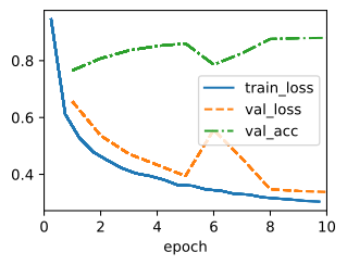
trainer = d2l.Trainer(max_epochs=10)
data = d2l.FashionMNIST(batch_size=128)
with d2l.try_gpu():
    model = BNLeNetScratch(lr=0.5)
    trainer.fit(model, data)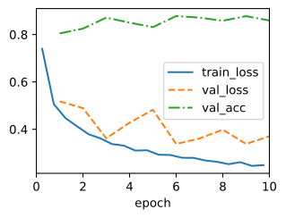
trainer = d2l.Trainer(max_epochs=10, num_gpus=1)
data = d2l.FashionMNIST(batch_size=128)
model = BNLeNetScratch(lr=0.1)
trainer.fit(model, data)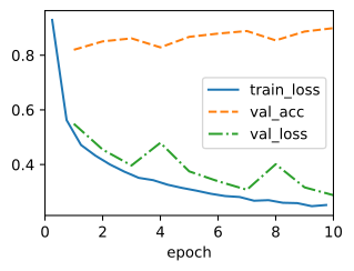
trainer = d2l.Trainer(max_epochs=10, num_gpus=1)
data = d2l.FashionMNIST(batch_size=128)
model = BNLeNetScratch(lr=0.1)
trainer.fit(model, data)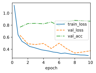
We inspect the scale parameter gamma and the shift parameter beta learned from the first batch normalization layer.
model.net[1].gamma.reshape((-1,)), model.net[1].beta.reshape((-1,))(tensor([1.4442, 2.0445, 1.7394, 1.9345, 2.1598, 1.9288], device='cuda:0',
grad_fn=<ViewBackward0>),
tensor([-1.0764, 0.8309, 1.6231, 0.8588, 0.9734, 1.3145], device='cuda:0',
grad_fn=<ViewBackward0>))tf.reshape(model.net.layers[1].gamma, (-1,)), tf.reshape(
model.net.layers[1].beta, (-1,))(<tf.Tensor: shape=(6,), dtype=float32, numpy=
array([2.6330233, 2.25818 , 3.374007 , 3.820023 , 2.5220754, 2.6115816],
dtype=float32)>,
<tf.Tensor: shape=(6,), dtype=float32, numpy=
array([ 2.1658266 , -2.5676103 , -1.7646055 , -2.344429 , 2.7539537 ,
-0.35519245], dtype=float32)>)model.net.layers[1].gamma[...].reshape((-1,)), \
model.net.layers[1].beta[...].reshape((-1,))(Array([2.6707244, 1.8966421, 1.8147523, 1.6768903, 1.9702979, 1.7232087], dtype=float32),
Array([ 1.2342167 , 0.5609814 , -0.26910412, 0.81538904, 0.20941882,
0.6389893 ], dtype=float32))model.net[1].gamma.data().reshape(-1,), model.net[1].beta.data().reshape(-1,)(array([1.7913003, 1.3728284, 1.0702729, 2.517021 , 1.7961818, 1.9894772], device=gpu(0)),
array([ 0.12360483, -0.8486686 , 0.8282237 , -1.5050275 , 1.1524508 ,
1.2504412 ], device=gpu(0)))7.3.5 Concise Implementation
Compared with the BatchNorm class, which we defined above, we can use the BatchNorm class defined in high-level APIs from the deep learning framework directly. The code looks virtually identical to our implementation above, except that we no longer need to provide additional arguments for it to get the dimensions right.
class BNLeNet(d2l.Classifier):
    def __init__(self, lr=0.1, num_classes=10):
        super().__init__()
        self.save_hyperparameters()
        self.net = nn.Sequential(
            nn.LazyConv2d(6, kernel_size=5), nn.LazyBatchNorm2d(),
            nn.Sigmoid(), nn.AvgPool2d(kernel_size=2, stride=2),
            nn.LazyConv2d(16, kernel_size=5), nn.LazyBatchNorm2d(),
            nn.Sigmoid(), nn.AvgPool2d(kernel_size=2, stride=2),
            nn.Flatten(), nn.LazyLinear(120), nn.LazyBatchNorm1d(),
            nn.Sigmoid(), nn.LazyLinear(84), nn.LazyBatchNorm1d(),
            nn.Sigmoid(), nn.LazyLinear(num_classes))
class BNLeNet(d2l.Classifier):
def __init__(self, lr=0.1, num_classes=10):
super().__init__()
self.save_hyperparameters()
self.net = tf.keras.models.Sequential([
tf.keras.Input(shape=(28, 28, 1)),
tf.keras.layers.Conv2D(filters=6, kernel_size=5),
tf.keras.layers.BatchNormalization(),
tf.keras.layers.Activation('sigmoid'),
tf.keras.layers.AvgPool2D(pool_size=2, strides=2),
tf.keras.layers.Conv2D(filters=16, kernel_size=5),
tf.keras.layers.BatchNormalization(),
tf.keras.layers.Activation('sigmoid'),
tf.keras.layers.AvgPool2D(pool_size=2, strides=2),
tf.keras.layers.Flatten(), tf.keras.layers.Dense(120),
tf.keras.layers.BatchNormalization(),
tf.keras.layers.Activation('sigmoid'),
tf.keras.layers.Dense(84),
tf.keras.layers.BatchNormalization(),
tf.keras.layers.Activation('sigmoid'),
tf.keras.layers.Dense(num_classes)])class BNLeNet(d2l.Classifier):
def __init__(self, lr=0.1, num_classes=10, rngs=None):
super().__init__()
self.save_hyperparameters(ignore=['rngs'])
rngs = nnx.Rngs(d2l.get_key()) if rngs is None else rngs
# Flax's default momentum=0.99 decays the OLD running stats; PT/MX use
# momentum=0.1 on the NEW stats, i.e. decay-of-OLD = 0.9. Pass 0.9 to
# match the other tabs.
self.net = nnx.Sequential(
nnx.Conv(1, 6, kernel_size=(5, 5), rngs=rngs),
nnx.BatchNorm(6, momentum=0.9, rngs=rngs), nnx.sigmoid,
lambda x: nnx.avg_pool(x, window_shape=(2, 2), strides=(2, 2)),
nnx.Conv(6, 16, kernel_size=(5, 5), rngs=rngs),
nnx.BatchNorm(16, momentum=0.9, rngs=rngs), nnx.sigmoid,
lambda x: nnx.avg_pool(x, window_shape=(2, 2), strides=(2, 2)),
lambda x: x.reshape((x.shape[0], -1)),
nnx.Linear(7 * 7 * 16, 120, rngs=rngs),
nnx.BatchNorm(120, momentum=0.9, rngs=rngs), nnx.sigmoid,
nnx.Linear(120, 84, rngs=rngs),
nnx.BatchNorm(84, momentum=0.9, rngs=rngs), nnx.sigmoid,
nnx.Linear(84, num_classes, rngs=rngs))class BNLeNet(d2l.Classifier):
def __init__(self, lr=0.1, num_classes=10):
super().__init__()
self.save_hyperparameters()
self.net = nn.Sequential()
self.net.add(
nn.Conv2D(6, kernel_size=5), nn.BatchNorm(),
nn.Activation('sigmoid'),
nn.AvgPool2D(pool_size=2, strides=2),
nn.Conv2D(16, kernel_size=5), nn.BatchNorm(),
nn.Activation('sigmoid'),
nn.AvgPool2D(pool_size=2, strides=2),
nn.Dense(120), nn.BatchNorm(), nn.Activation('sigmoid'),
nn.Dense(84), nn.BatchNorm(), nn.Activation('sigmoid'),
nn.Dense(num_classes))
self.initialize()Below, we use the same hyperparameters to train our model. Note that as usual, the high-level API variant runs much faster because its code has been compiled to C++ or CUDA while our custom implementation must be interpreted by Python.
trainer = d2l.Trainer(max_epochs=10, num_gpus=1)
data = d2l.FashionMNIST(batch_size=128)
model = BNLeNet(lr=0.1)
model.apply_init([next(iter(data.get_dataloader(True)))[0]], d2l.init_cnn)
trainer.fit(model, data)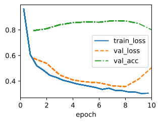
trainer = d2l.Trainer(max_epochs=10)
data = d2l.FashionMNIST(batch_size=128)
with d2l.try_gpu():
    model = BNLeNet(lr=0.5)
    trainer.fit(model, data)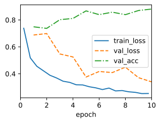
trainer = d2l.Trainer(max_epochs=10, num_gpus=1)
data = d2l.FashionMNIST(batch_size=128)
model = BNLeNet(lr=0.1)
trainer.fit(model, data)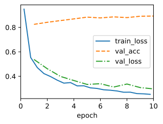
trainer = d2l.Trainer(max_epochs=10, num_gpus=1)
data = d2l.FashionMNIST(batch_size=128)
model = BNLeNet(lr=0.1)
trainer.fit(model, data)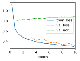
7.3.6 Beyond Batch Normalization
Batch normalization is unusual among the layers in this book: its output for one example depends on the other examples in the minibatch. That coupling is where the regularizing noise comes from, and it is also where the practical trouble comes from. Two problems recur.
The first is minibatch coupling. The estimates \(\hat{\boldsymbol{\mu}}_{\mathcal{B}}\) and \(\hat{\boldsymbol{\sigma}}_{\mathcal{B}}\) stand and fall with the batch size: we saw above that a fully connected layer learns nothing at batch size 1 and that very small batches make the statistics unreliable. This bites hardest in dense prediction. Object detection and semantic segmentation train on high-resolution images, so memory often limits the batch to one or two images per device, exactly where batch statistics are noisiest.
The second is the train/serve discrepancy. As discussed above, the layer applies minibatch statistics during training but moving averages at prediction time, so the network computes two different functions depending on the mode. Whenever the moving averages summarize the served data poorly, for instance after fine-tuning on a new domain or when a bug freezes them, accuracy drops in ways that are hard to trace back to a normalization layer.
7.3.6.1 Group Normalization
Group normalization (Wu and He 2018) removes the batch from the statistics. It divides the \(c\) channels into \(G\) groups of \(c/G\) channels and standardizes each example separately over each group, i.e., over \((c/G) \cdot p \cdot q\) elements, again followed by a per-channel scale \(\boldsymbol{\gamma}\) and shift \(\boldsymbol{\beta}\) as in Equation 7.3.1. Setting \(G=1\) normalizes each example over all channels and positions at once; setting \(G=c\) normalizes every channel separately (a variant known as instance normalization). Intermediate group counts such as \(G=32\) tend to work best: enough elements per group for stable statistics, without forcing unrelated channels to share them.
Because no other example enters the statistics, group normalization computes the same function at batch size 1 as at batch size 32, and the same function during training as at prediction time; there are no moving averages to maintain. The code below checks both claims: after group normalization, every (example, group) pair has mean 0 and variance 1, and normalizing an example alone gives the same output as normalizing it inside a batch.
X = torch.randn(32, 16, 8, 8)
gn = nn.GroupNorm(4, 16)  # 4 groups of 4 channels each
Y = gn(X)
G = Y.reshape(32, 4, -1)  # Collect each (example, group) pair's elements
(G.mean(dim=2).abs().max(), G.var(dim=2, unbiased=False).mean(),
 torch.allclose(gn(X[:1]), Y[:1], atol=1e-6))
(tensor(2.4214e-08, grad_fn=<MaxBackward1>),
tensor(1.0000, grad_fn=<MeanBackward0>),
True)X = tf.random.normal((32, 8, 8, 16)) # Channels last, as Keras expects
gn = tf.keras.layers.GroupNormalization(groups=4) # Groups the last axis
Y = gn(X)
# Collect each (example, group) pair's elements
G = tf.reshape(tf.transpose(Y, (0, 3, 1, 2)), (32, 4, -1))
(tf.reduce_max(tf.abs(tf.reduce_mean(G, axis=2))),
tf.reduce_mean(tf.math.reduce_variance(G, axis=2)),
bool(tf.reduce_all(tf.abs(gn(X[:1]) - Y[:1]) < 1e-5)))(<tf.Tensor: shape=(), dtype=float32, numpy=2.60770320892334e-08>,
<tf.Tensor: shape=(), dtype=float32, numpy=0.9989977478981018>,
True)X = jax.random.normal(jax.random.PRNGKey(0), (32, 8, 8, 16)) # Channels last
gn = nnx.GroupNorm(16, num_groups=4, rngs=nnx.Rngs(1))
Y = gn(X)
# Collect each (example, group) pair's elements
G = jnp.transpose(Y, (0, 3, 1, 2)).reshape(32, 4, -1)
(jnp.abs(G.mean(axis=2)).max(), G.var(axis=2).mean(),
jnp.allclose(gn(X[:1]), Y[:1], atol=1e-6))(Array(2.6077032e-08, dtype=float32),
Array(0.999999, dtype=float32),
Array(True, dtype=bool))X = np.random.normal(size=(32, 16, 8, 8))
gn = nn.GroupNorm(num_groups=4) # 4 groups of 4 channels each
gn.initialize()
Y = gn(X)
G = Y.reshape(32, 4, -1) # Collect each (example, group) pair's elements
(np.abs(G.mean(axis=2)).max(), G.var(axis=2).mean(),
bool(np.abs(gn(X[:1]) - Y[:1]).max() < 1e-5))(array(2.9802322e-08), array(0.9999898), True)The trade-off runs in the other direction too: with large batches, batch normalization averages over more elements and keeps a small accuracy edge on ImageNet classification, but as the batch shrinks below roughly eight examples per device its accuracy degrades quickly while group normalization is unaffected (Wu and He 2018). Group normalization is therefore the default in detection and segmentation heads and in diffusion U-Nets, settings where large per-device batches are unaffordable.
7.3.6.2 Layer Normalization in Convolutional Networks
Layer normalization from Section 7.3.2.3 is the other batch-free option, and modern convolutional networks use it in a specific form: at every spatial position, normalize the \(c\) channel values at that position, just as a transformer normalizes each token’s embedding. ConvNeXt, a convolutional architecture we will meet later in this chapter, makes exactly this choice: it replaces every batch normalization in a ResNet-style network with per-position, channels-last layer normalization, uses fewer normalization layers overall, and loses no accuracy in the process (Section 7.7).
7.3.6.3 Normalizer-Free Networks
One can push further and ask whether deep networks need normalization layers at all. Normalizer-free networks (NFNets) (Brock et al. 2021) answer no. They train ResNet-style networks that held the ImageNet state of the art at publication, with no normalization anywhere, by combining weight standardization (standardizing each convolution’s weights rather than its activations) with adaptive gradient clipping (clipping a unit’s gradient when its norm grows large relative to the corresponding weight norm). Dropping batch normalization eliminates minibatch coupling and the train/serve discrepancy in one stroke, and it removes the cost of computing batch statistics on large activations. We return to normalizer-free networks when we discuss scaling up convolutional networks in Section 7.8.
7.3.7 Discussion
Intuitively, batch normalization is thought to make the optimization landscape smoother. However, we must be careful to distinguish between speculative intuitions and true explanations for the phenomena that we observe when training deep models. Recall that we do not even know why simpler deep neural networks (MLPs and conventional CNNs) generalize well in the first place. Even with dropout and weight decay, they remain so flexible that their ability to generalize to unseen data likely needs significantly more refined learning-theoretic generalization guarantees.
The original batch-normalization paper (Ioffe and Szegedy 2015) also offered an explanation for why it works: by reducing internal covariate shift. Presumably by internal covariate shift they meant something like the intuition expressed above—the notion that the distribution of variable values changes over the course of training. However, there were two problems with this explanation: i) This drift is very different from covariate shift, rendering the name a misnomer. If anything, it is closer to concept drift. ii) The explanation offers an under-specified intuition but leaves the question of why precisely this technique works an open question wanting for a rigorous explanation. Throughout this book, we aim to convey the intuitions that practitioners use to guide their development of deep neural networks. However, we believe that it is important to separate these guiding intuitions from established scientific fact. Eventually, when you master this material and start writing your own research papers you will want to be clear to delineate between technical claims and hunches.
Following the success of batch normalization, its explanation in terms of internal covariate shift has repeatedly surfaced in debates in the technical literature and broader discourse about how to present machine learning research. In a memorable speech given while accepting a Test of Time Award at the 2017 NeurIPS conference, Ali Rahimi used internal covariate shift as a focal point in an argument likening the modern practice of deep learning to alchemy. Subsequently, the example was revisited in detail in a position paper outlining troubling trends in machine learning (Lipton and Steinhardt 2018). Other authors have proposed alternative explanations for the success of batch normalization, some (Santurkar et al. 2018) claiming that batch normalization succeeds despite behavior that is in some ways the opposite of what the original paper claimed.
We note that the internal covariate shift is no more worthy of criticism than any of thousands of similarly vague claims made every year in the technical machine learning literature. It likely became a focal point of these debates because it was so broadly recognizable to the target audience. Batch normalization became a standard component of convolutional classifiers, while GroupNorm, LayerNorm, and normalizer-free networks now cover regimes in which batch statistics are undesirable. The competing explanations remain a useful case study in separating an empirical result from its proposed mechanism.
The practical points are:
- During model training, batch normalization continuously adjusts the intermediate output of the network by utilizing the mean and standard deviation of the minibatch, so that the values of the intermediate output in each layer throughout the neural network are more stable.
- Batch normalization is slightly different for fully connected layers than for convolutional layers. In fact, for convolutional layers, layer normalization can sometimes be used as an alternative.
- Like a dropout layer, batch normalization layers have different behaviors in training mode than in prediction mode.
- Batch normalization is useful for regularization and improving convergence in optimization. By contrast, the original motivation of reducing internal covariate shift seems not to be a valid explanation.
- For more robust models that are less sensitive to input perturbations, consider removing batch normalization (Wang et al. 2022).
7.3.8 Exercises
- Bias before batch norm. Should we remove the bias parameter from the fully connected layer or the convolutional layer before the batch normalization? Justify your answer from Equation 7.3.1.
- [code] Learning-rate ceiling. Compare
LeNet(Section 6.6) withBNLeNet.- Train both at the learning rate used in this section and plot validation accuracy against epoch.
- Increase the learning rate for both models until training fails, that is, until the loss diverges or accuracy stays at chance. How large a learning rate does each model tolerate?
- [code] Leave-one-out ablation. Does every layer need batch normalization?
BNLeNetnormalizes the output of each of its four hidden layers. Remove batch normalization from one layer at a time and retrain. Report, as a table, the validation-accuracy cost of each removal, and identify the layer whose removal hurts most. - [code] Batch norm lite. Implement a version of batch normalization that only removes the mean, and a second variant that only divides by the standard deviation. Compare the training curves and final accuracy of both against full batch normalization.
- [code] Frozen scale and shift. In every
BatchNormlayer ofBNLeNetScratch, hold the scalegammaand the shiftbetaconstant instead of learning them. Retrain twice: once with every entry of \(\boldsymbol{\gamma}\) equal to 1 and of \(\boldsymbol{\beta}\) equal to 0, which makes the affine map the identity, and once with every entry of \(\boldsymbol{\gamma}\) equal to 0.1 and of \(\boldsymbol{\beta}\) equal to 1. Compare the training-loss curves and the final validation accuracy of both runs with those ofBNLeNetScratchwith learnedgammaandbeta. Explain each difference you observe, or why none appears. - [code] Replacing dropout.
LeNet(Section 6.6) uses neither dropout nor batch normalization. Build a dropout variant ofLeNetthat adds dropout with rate 0.5 after each of its two hidden fully connected layers. TrainLeNet, the dropout variant, andBNLeNet, which inserts batch normalization instead, for the same number of epochs. Report the validation accuracy of each network and the gap between its training and validation accuracy. Does each addition narrow or widen the gap ofLeNet? Explain the result forBNLeNet. - [code] Minibatch coupling. The output of batch normalization for one example depends on the other examples in its minibatch. Train
BNLeNetScratchas in this section. Measure its validation accuracy in prediction mode, then in training mode with validation batches of 128 images, and then in training mode with validation batches of one image. Measure in prediction mode first, since every training-mode forward pass updates the moving averages. Explain the three accuracies. - [code] Small-batch training. ● Build a variant of
BNLeNetthat uses group normalization with two groups after each convolutional layer and layer normalization (Section 7.3.2.3) after each hidden fully connected layer, in place of batch normalization. TrainBNLeNetand the variant for two epochs at batch size 4 and again at batch size 128, keeping the other hyperparameters of this section. Report the validation accuracy of all four runs. How does the accuracy of each network change when the batch size drops from 128 to 4, and why? - [code] Backward pass of batch norm. ● The batch statistics in Equation 7.3.1 depend on every element of the minibatch, so the backward pass is not elementwise.
- Derive, by hand, the gradient of a scalar loss with respect to each input of the batch-norm layer, working through the forward steps: mean, centering, variance, normalization, and the affine scale and shift.
- Implement your expression and verify it against the gradient computed by automatic differentiation.
- [extended] Beyond mean and variance. ●● Batch normalization standardizes each channel separately. For each of the following alternatives, describe how it would be applied at a layer and what it costs in computation, parameters, and estimation variance. Implement at least one of them in place of
BatchNorminBNLeNetScratchand compare its validation accuracy with that of batch normalization.- The probability integral transform, which maps each channel through its empirical cumulative distribution function.
- Whitening with a full covariance estimate across the \(c\) channels.
- Whitening with a structured covariance estimate, for example a block-diagonal or a low-rank-plus-diagonal matrix.