%matplotlib inline
from d2l import torch as d2l
import gymnasium as gym
import numpy as np
import torch
from torch import nn
torch.set_num_threads(1)15.6 Learned Models and Planning
Soft actor-critic swung the pendulum up after a few thousand transitions, and it used every transition in the same way: as the target of one regression for its critic, a reward plus the discounted value of the next state. A transition records more than that. It shows how the pendulum moved under a particular torque, and the physics behind that motion is the same at every visit. A child who has been pushed on a swing a few times can say where the swing will be a moment later and how hard to push to send it higher. Could an agent learn the physics of the pendulum from a few hundred steps and plan its way up, with no critic and no policy?
Section 14.3 did this on the lake. It counted the transitions it had seen into an estimated model and ran value iteration on the estimate, treating it as exact. Pendulum’s states are continuous, so they cannot be counted. Regression takes the place of counting: a network learns to predict the next state and the reward from the current state and the torque. Search takes the place of value iteration: the agent tries many torque sequences inside the model and executes the first torque of the best one. Sutton’s Dyna architecture combined a learned model with planning in 1990 (Sutton 1990), and neural-network models searched in this way control simulated robots from minutes of experience (Nagabandi et al. 2018).
A model lets an agent use computation in place of experience: every real step can be followed by thousands of imagined ones. A search can also start from what a policy proposes and teach its result back to the policy. AlphaZero and MuZero learned to play board games beyond human strength in this way (Silver et al. 2018; Schrittwieser et al. 2020), and search guided by a learned policy is one way language models spend extra computation at test time. In this section we fit a model of Pendulum from one random episode, measure how its errors grow along a plan, plan with it, and turn the search into a better policy. One question stays with us throughout: how far from its data can a model be trusted?
%matplotlib inline
from d2l import jax as d2l
from flax import nnx
import gymnasium as gym
import jax
from jax import numpy as jnp
import numpy as np
import optax
15.6.1 A Dynamics Model from Data
15.6.1.1 Regression in Place of Counting
Pendulum is the task of Section 15.5. A pendulum hangs from a motorized pivot; the state is \(s = (\cos\vartheta, \sin\vartheta, \dot\vartheta)\), where \(\vartheta\) is the angle from upright, and the action is a torque \(a \in [-2, 2]\). Each step gives the reward \(-(\vartheta^2 + 0.1\,\dot\vartheta^2 + 0.001\,a^2)\) with \(\vartheta\) wrapped to \([-\pi, \pi]\), and an episode lasts 200 steps. A pendulum hanging still at the bottom loses \(\pi^2 \approx 9.9\) per step, about \(2{,}000\) per episode; random torques lose about \(900\) to \(1{,}700\); a controller that swings the pendulum up and balances it loses between zero and a few hundred, depending on where it starts.
A model of the environment predicts what the environment does. We write \(\hat f_\phi\) for a network with parameters \(\phi\) that maps a state and an action to a predicted next state and reward,
\[(\hat s', \hat r) = \hat f_\phi(s, a). \tag{15.6.1}\]
On the lake the model was a table of frequencies, and every entry was estimated only from the visits to its own state-action pair. A network shares its parameters across states, so a transition at one angle also teaches the model about nearby angles. We fit it by least squares on the stored transitions \((s_i, a_i, r_i, s'_i)\),
\[ \min_\phi \sum_i \big\| \hat f_\phi(s_i, a_i) - (s'_i, r_i) \big\|^2. \tag{15.6.2}\]
The fit asks the model to reproduce the recorded next state and reward of every stored transition. With a table in place of the network, the minimizer at each pair would be the average of the outcomes observed there: the counted model of Section 14.3, reduced to its mean. Pendulum is deterministic, so the mean outcome is the outcome. A stochastic environment would need a model of the whole distribution of next states, as the counts provided on the lake.
Two choices make the regression easy. The network predicts the change of state \(s' - s\) rather than \(s'\) itself, because in one step of 0.05 seconds the pendulum moves only a little, and the change is the part worth learning. And every input and target coordinate is standardized to mean zero and variance one over the stored data, because the coordinates live on different scales: the cosine and sine lie in \([-1, 1]\), the angular velocity in \([-8, 8]\), and the reward in about \([-16, 0]\). Without standardization least squares would mostly fit the reward.
The settings for the whole section come first: the torque bound \(c = 2\), the depth \(n = 25\) of a plan, the number of candidate plans the search tries, the number of Adam steps per fit of the model, the number of seeds, and the seed that fixes the starting states of our test.
c, horizon, num_cand = 2.0, 25, 500   # torque bound, depth n, candidates
fit_steps, num_seeds, test_seed = 1_000, 5, 1_000
c, horizon, num_cand = 2.0, 25, 500 # torque bound, depth n, candidates
fit_steps, num_seeds, test_seed = 1_000, 5, 1_000Data come from whole episodes. run_episode acts in a vector environment, gymnasium’s container that steps several copies of Pendulum in lockstep, so that one call can run a controller from ten starting states at once. A controller is any function from a batch of observations to a batch of actions, and random_controller returns one that draws uniformly random torques. score runs a controller for one episode from ten fixed starts, those of environment seeds 1000 to 1009, and returns the mean return; it is the test for every controller in this section. The transitions go into a d2l.ReplayBufferC, the replay buffer of Section 15.5 with a floating-point action column. Here it serves only as a store of arrays; we never sample batches from it. model_data turns the stored transitions into the inputs \((s, a)\) and targets \((s' - s, r)\) of the regression, with their means and standard deviations.
def run_episode(envs, controller, buffer=None, seed=None, num_steps=200):
    """One episode in every environment of a vector env, acting by
    controller(obs) -> actions. Returns the returns; records transitions."""
    obs, total = envs.reset(seed=seed)[0], 0.0
    for _ in range(num_steps):
        act = controller(obs)
        next_obs, rew, term, _, _ = envs.step(act)
        for i in range(envs.num_envs if buffer is not None else 0):
            buffer.add(obs[i], act[i], rew[i], next_obs[i], float(term[i]))
        obs, total = next_obs, total + rew
    return total

def random_controller(rng, scale=c):
    """Uniformly random torques: the data of the first episode."""
    return lambda obs: rng.uniform(-scale, scale, (len(obs), 1)).astype(
        np.float32)

def score(controller, num_starts=10, seed=test_seed):
    """Mean return of a controller over ten fixed Pendulum starts."""
    envs = gym.make_vec('Pendulum-v1', num_envs=num_starts,
                        vectorization_mode='sync')
    return run_episode(envs, controller, seed=seed).mean()

def model_data(buffer):
    """Inputs (s, a) and targets (s' - s, r) of the stored transitions,
    with their means and standard deviations."""
    n = buffer.size
    x = np.concatenate([buffer.obs[:n], buffer.act[:n]], -1)
    y = np.concatenate([buffer.next_obs[:n] - buffer.obs[:n],
                        buffer.rew[:n, None]], -1)
    return x, y, (x.mean(0), x.std(0) + 1e-6, y.mean(0), y.std(0) + 1e-6)
def run_episode(envs, controller, buffer=None, seed=None, num_steps=200):
"""One episode in every environment of a vector env, acting by
controller(obs) -> actions. Returns the returns; records transitions."""
obs, total = envs.reset(seed=seed)[0], 0.0
for _ in range(num_steps):
act = controller(obs)
next_obs, rew, term, _, _ = envs.step(act)
for i in range(envs.num_envs if buffer is not None else 0):
buffer.add(obs[i], act[i], rew[i], next_obs[i], float(term[i]))
obs, total = next_obs, total + rew
return total
def random_controller(rng, scale=c):
"""Uniformly random torques: the data of the first episode."""
return lambda obs: rng.uniform(-scale, scale, (len(obs), 1)).astype(
np.float32)
def score(controller, num_starts=10, seed=test_seed):
"""Mean return of a controller over ten fixed Pendulum starts."""
envs = gym.make_vec('Pendulum-v1', num_envs=num_starts,
vectorization_mode='sync')
return run_episode(envs, controller, seed=seed).mean()
def model_data(buffer):
"""Inputs (s, a) and targets (s' - s, r) of the stored transitions,
with their means and standard deviations."""
n = buffer.size
x = np.concatenate([buffer.obs[:n], buffer.act[:n]], -1)
y = np.concatenate([buffer.next_obs[:n] - buffer.obs[:n],
buffer.rew[:n, None]], -1)
return x, y, (x.mean(0), x.std(0) + 1e-6, y.mean(0), y.std(0) + 1e-6)DynamicsModel is a multilayer perceptron with two hidden layers of 64 units and the smooth SiLU activation (Section 4.1). It holds the standardization statistics in stats; its forward pass standardizes the input, undoes the standardization of the output, and adds the predicted change to the state. fit_model recomputes the statistics from all stored data, then takes Adam steps on minibatches of 256 transitions. Its optimizer is created once with the model, in make_model, so each later fit continues from the previous parameters instead of starting over.
class DynamicsModel(nn.Module):
    """(s', r) from (s, a): an MLP that maps standardized inputs to the
    standardized change of state and reward."""
    def __init__(self, obs_dim=3, act_dim=1, hidden=64):
        super().__init__()
        d_in, d_out = obs_dim + act_dim, obs_dim + 1
        self.net = nn.Sequential(nn.Linear(d_in, hidden), nn.SiLU(),
                                 nn.Linear(hidden, hidden), nn.SiLU(),
                                 nn.Linear(hidden, d_out))
        self.stats = (torch.zeros(d_in), torch.ones(d_in),
                      torch.zeros(d_out), torch.ones(d_out))

    def forward(self, obs, act):
        mu_x, sd_x, mu_y, sd_y = self.stats
        x = (torch.cat([obs, act], -1) - mu_x) / sd_x
        y = self.net(x) * sd_y + mu_y          # (s' - s, r) in data units
        return obs + y[..., :-1], y[..., -1]

def make_model(seed, lr=1e-3):
    torch.manual_seed(seed)
    model = DynamicsModel()
    return model, torch.optim.Adam(model.parameters(), lr=lr)

def fit_model(model, opt, buffer, rng, num_steps=fit_steps, batch_size=256):
    """Least squares on all stored transitions, in standardized units."""
    x, y, stats = model_data(buffer)
    model.stats = tuple(torch.as_tensor(v) for v in stats)
    mu_x, sd_x, mu_y, sd_y = stats
    x = torch.as_tensor((x - mu_x) / sd_x)
    y = torch.as_tensor((y - mu_y) / sd_y)
    for _ in range(num_steps):
        i = torch.as_tensor(rng.integers(len(x), size=batch_size))
        loss = ((model.net(x[i]) - y[i]) ** 2).mean()
        opt.zero_grad()
        loss.backward()
        opt.step()
    return float(loss.detach())
class DynamicsModel(nnx.Module):
"""(s', r) from (s, a): an MLP that maps standardized inputs to the
standardized change of state and reward."""
def __init__(self, obs_dim=3, act_dim=1, hidden=64, rngs=None):
d_in, d_out = obs_dim + act_dim, obs_dim + 1
self.net = nnx.Sequential(
d2l.Linear(d_in, hidden, rngs=rngs), jax.nn.silu,
d2l.Linear(hidden, hidden, rngs=rngs), jax.nn.silu,
d2l.Linear(hidden, d_out, rngs=rngs))
self.stats = nnx.Variable((jnp.zeros(d_in), jnp.ones(d_in),
jnp.zeros(d_out), jnp.ones(d_out)))
def __call__(self, obs, act):
mu_x, sd_x, mu_y, sd_y = self.stats.get_value()
x = (jnp.concatenate([obs, act], -1) - mu_x) / sd_x
y = self.net(x) * sd_y + mu_y # (s' - s, r) in data units
return obs + y[..., :-1], y[..., -1]
def make_model(seed, lr=1e-3):
model = DynamicsModel(rngs=nnx.Rngs(seed))
return model, nnx.Optimizer(model, optax.adam(lr), wrt=nnx.Param)
@nnx.jit
def model_step(model, opt, x, y):
loss = lambda m: ((m.net(x) - y) ** 2).mean()
value, grads = nnx.value_and_grad(loss)(model)
opt.update(model, grads)
return value
def fit_model(model, opt, buffer, rng, num_steps=fit_steps, batch_size=256):
"""Least squares on all stored transitions, in standardized units."""
x, y, stats = model_data(buffer)
model.stats.set_value(tuple(jnp.asarray(v) for v in stats))
mu_x, sd_x, mu_y, sd_y = stats
x, y = (x - mu_x) / sd_x, (y - mu_y) / sd_y
step = nnx.cached_partial(model_step, model, opt)
for _ in range(num_steps):
i = rng.integers(len(x), size=batch_size)
loss = step(x[i], y[i])
return float(loss)The layers are d2l.Linear, the initialization used for every JAX network in these two chapters (Section 14.8). The statistics live in an nnx.Variable, so the compiled functions below read their current values after every refit. model_step is one compiled Adam step, and nnx.cached_partial binds the model and the optimizer to it once per fit.
We collect one episode of random torques from seed 0 and fit the model to its 200 transitions:
env = gym.make_vec('Pendulum-v1', num_envs=1, vectorization_mode='sync')
rng = np.random.default_rng(0)
buffer = d2l.ReplayBufferC(200, 3, 1)
print(f'return of the random episode: '
      f'{run_episode(env, random_controller(rng), buffer, seed=0)[0]:.0f}')
model, opt = make_model(0)
print(f'final minibatch loss (standardized units): '
      f'{fit_model(model, opt, buffer, rng):.4f}')
return of the random episode: -1072
final minibatch loss (standardized units): 0.0018env = gym.make_vec('Pendulum-v1', num_envs=1, vectorization_mode='sync')
rng = np.random.default_rng(0)
buffer = d2l.ReplayBufferC(200, 3, 1)
print(f'return of the random episode: '
f'{run_episode(env, random_controller(rng), buffer, seed=0)[0]:.0f}')
model, opt = make_model(0)
print(f'final minibatch loss (standardized units): '
f'{fit_model(model, opt, buffer, rng):.4f}')return of the random episode: -1072
final minibatch loss (standardized units): 0.0013The random episode loses about a thousand, and the loss at the end of the fit is a small fraction of the targets’ variance, which is one in standardized units.
15.6.1.2 One Step by Hand
A small training loss does not tell us what the model predicts. We look at one transition of the episode in the units of the problem. rollout_model feeds a state and a sequence of actions through the model, each predicted state becoming the input of the next step; with a single action it is one prediction.
@torch.no_grad()
def rollout_model(model, obs, actions):
    """Open-loop rollout in the model: obs (..., 3) and actions (..., n, 1)
    give the predicted states (..., n, 3) and rewards (..., n)."""
    s, actions = torch.as_tensor(obs), torch.as_tensor(actions)
    states, rewards = [], []
    for t in range(actions.shape[-2]):
        s, r = model(s, actions[..., t, :])
        states.append(s)
        rewards.append(r)
    return torch.stack(states, -2).numpy(), torch.stack(rewards, -1).numpy()
@nnx.jit
def rollout_model(model, obs, actions):
"""Open-loop rollout in the model: obs (..., 3) and actions (..., n, 1)
give the predicted states (..., n, 3) and rewards (..., n)."""
def step(s, a):
s, r = model(s, a)
return s, (s, r)
_, (states, rewards) = jax.lax.scan(step, obs,
jnp.moveaxis(actions, -2, 0))
return jnp.moveaxis(states, 0, -2), jnp.moveaxis(rewards, 0, -1)rollout_model runs the steps with jax.lax.scan under nnx.jit; it compiles once for every shape of its inputs, and the section calls it with only a few shapes.
def angle(s):
    """Angle from upright in degrees, from states (cos, sin, velocity)."""
    return np.degrees(np.arctan2(s[..., 1], s[..., 0]))

i = 100
pred, r_hat = rollout_model(model, buffer.obs[i], buffer.act[i][None])
print('s       ', buffer.obs[i].round(4), f'a = {buffer.act[i, 0]:.4f}')
print("true s' ", buffer.next_obs[i].round(4), f'r = {buffer.rew[i]:.4f}')
print("model s'", np.asarray(pred[0]).round(4),
      f'r = {float(r_hat[0]):.4f}')
print(f'angle error {abs(angle(pred[0]) - angle(buffer.next_obs[i])):.3f} '
      f'degrees')
s [-0.9407 -0.3394 5.6896] a = -0.0800
true s' [-0.8154 -0.5789 5.4231] r = -11.0511
model s' [-0.8109 -0.584 5.436 ] r = -11.2768
angle error 0.386 degreesdef angle(s):
"""Angle from upright in degrees, from states (cos, sin, velocity)."""
return np.degrees(np.arctan2(s[..., 1], s[..., 0]))
i = 100
pred, r_hat = rollout_model(model, buffer.obs[i], buffer.act[i][None])
print('s ', buffer.obs[i].round(4), f'a = {buffer.act[i, 0]:.4f}')
print("true s' ", buffer.next_obs[i].round(4), f'r = {buffer.rew[i]:.4f}')
print("model s'", np.asarray(pred[0]).round(4),
f'r = {float(r_hat[0]):.4f}')
print(f'angle error {abs(angle(pred[0]) - angle(buffer.next_obs[i])):.3f} '
f'degrees')s [-0.9407 -0.3394 5.6896] a = -0.0800
true s' [-0.8154 -0.5789 5.4231] r = -11.0511
model s' [-0.8115 -0.5825 5.4327] r = -11.1913
angle error 0.295 degreesAt step 100 the pendulum is at \(\vartheta = \operatorname{atan2}(-0.3394, -0.9407) = -2.795\) radians, about \(160\) degrees from upright, and it swings at \(5.69\) radians per second while the torque is nearly zero. The reward is \(-(2.795^2 + 0.1 \cdot 5.690^2 + 0.001 \cdot 0.08^2) = -11.05\), as printed. In the 0.05 seconds of one step the angle moves to \(\operatorname{atan2}(-0.5789, -0.8154) = -144.6\) degrees, about \(5.6 \times 0.05 = 0.28\) radians or 16 degrees, and the model predicts this move to within a fraction of a degree. Its reward is off by less than three tenths. One step is easy: it is a small correction of a state the model has just been shown.
15.6.1.3 Compounding Error
A plan needs more than one step. To score a sequence of torques the model must predict 25 steps ahead, and from the second step on its input is its own previous prediction. The model was trained only on true states, never on its own slightly wrong ones, so an error at one step changes the input of the next: a small error in the angle changes the torque that gravity exerts, which changes the velocity, which changes the angle further. We measure this with open-loop rollouts, which follow the actions recorded in an episode while the model predicts the states, and we compare the predicted angle after \(k\) steps with the recorded one.
kstep_error starts a rollout at every step of an episode that leaves 25 steps before the end, and reports the root-mean-square error of the angle after \(k = 1, 5, 10, 25\) steps, wrapped so that \(+179\) and \(-179\) degrees are two degrees apart.
def kstep_error(model, buffer, first=0, ks=(1, 5, 10, 25), T=200):
    """RMS angle error (degrees) of open-loop model rollouts along the
    recorded actions, from every step of the stored T-step episodes (rows
    first onward) that leaves max(ks) steps before the episode ends."""
    n = max(ks)
    ep = lambda x: x[first:buffer.size].reshape(-1, T, *x.shape[1:])
    obs, act, nxt = ep(buffer.obs), ep(buffer.act), ep(buffer.next_obs)
    windows = lambda x: np.stack([x[:, t:t + n]
                                  for t in range(T - n + 1)], 1)
    pred = np.asarray(rollout_model(model, obs[:, :T - n + 1],
                                    windows(act))[0])
    d = np.radians(angle(pred) - angle(windows(nxt)))
    d = np.arctan2(np.sin(d), np.cos(d))         # wrapped to (-pi, pi]
    return [np.degrees(np.sqrt(np.mean(d[..., k - 1] ** 2))) for k in ks]
def kstep_error(model, buffer, first=0, ks=(1, 5, 10, 25), T=200):
"""RMS angle error (degrees) of open-loop model rollouts along the
recorded actions, from every step of the stored T-step episodes (rows
first onward) that leaves max(ks) steps before the episode ends."""
n = max(ks)
ep = lambda x: x[first:buffer.size].reshape(-1, T, *x.shape[1:])
obs, act, nxt = ep(buffer.obs), ep(buffer.act), ep(buffer.next_obs)
windows = lambda x: np.stack([x[:, t:t + n]
for t in range(T - n + 1)], 1)
pred = np.asarray(rollout_model(model, obs[:, :T - n + 1],
windows(act))[0])
d = np.radians(angle(pred) - angle(windows(nxt)))
d = np.arctan2(np.sin(d), np.cos(d)) # wrapped to (-pi, pi]
return [np.degrees(np.sqrt(np.mean(d[..., k - 1] ** 2))) for k in ks]For each of five seeds we fit a model to one random episode and test it on a second random episode from the same seed:
models = []
print('seed   k=1    k=5   k=10   k=25   (degrees, held-out random episode)')
for seed in range(num_seeds):
    rng = np.random.default_rng(seed)
    train, test = d2l.ReplayBufferC(200, 3, 1), d2l.ReplayBufferC(200, 3, 1)
    run_episode(env, random_controller(rng), train, seed=seed)
    run_episode(env, random_controller(rng), test)
    m, o = make_model(seed)
    fit_model(m, o, train, rng)
    models.append((m, test))
    errors = kstep_error(m, test)
    print(f'{seed:4d} ' + ' '.join(f'{e:6.2f}' for e in errors))
seed k=1 k=5 k=10 k=25 (degrees, held-out random episode)
0 0.44 1.91 2.52 1.51
1 1.83 7.08 8.67 12.29
2 0.53 2.37 3.65 5.51
3 0.38 1.89 4.77 11.82
4 0.04 0.12 0.13 0.33models = []
print('seed k=1 k=5 k=10 k=25 (degrees, held-out random episode)')
for seed in range(num_seeds):
rng = np.random.default_rng(seed)
train, test = d2l.ReplayBufferC(200, 3, 1), d2l.ReplayBufferC(200, 3, 1)
run_episode(env, random_controller(rng), train, seed=seed)
run_episode(env, random_controller(rng), test)
m, o = make_model(seed)
fit_model(m, o, train, rng)
models.append((m, test))
errors = kstep_error(m, test)
print(f'{seed:4d} ' + ' '.join(f'{e:6.2f}' for e in errors))seed k=1 k=5 k=10 k=25 (degrees, held-out random episode)
0 0.22 0.82 1.15 3.33
1 1.40 4.83 6.87 15.09
2 0.61 2.75 4.12 4.02
3 0.44 1.61 2.56 6.04
4 0.03 0.11 0.19 0.30On every seed the error after ten steps is several times the error after one step, and after one step it is a fraction of a degree on most seeds. After 25 steps the error depends on the seed, but on these held-out episodes it stays below about 20 degrees: under random torques the pendulum keeps swinging near the bottom, where the training episode went too. We return to this proviso after the planner has taken the pendulum elsewhere.
The depth of a plan is a dial like the \(n\) of the \(n\)-step returns in Section 15.1. A deeper plan sees further consequences of a torque; a swing-up takes a few dozen steps, and a plan that ends before the pendulum rises cannot tell a good pumping sequence from a bad one. But each further step adds the model’s error to the prediction. We use \(n = 25\) steps, 1.25 seconds, and exercise 1 moves the dial.
15.6.2 Planning in the Model
15.6.2.1 Random Shooting
Inside the model, trying a sequence of torques costs a few matrix multiplications and no real step. The simplest search uses this directly. Suppose the pendulum hangs still at the bottom. We draw five random sequences of 25 torques, roll each out in the model fitted above, and add up its predicted rewards:
rng = np.random.default_rng(0)
s = np.array([[-1.0, 0.0, 0.0]], np.float32)      # hanging down, at rest
A = rng.uniform(-c, c, (1, 5, horizon, 1)).astype(np.float32)
_, r_hat = rollout_model(model, np.repeat(s[:, None], 5, axis=1), A)
real = gym.make('Pendulum-v1').unwrapped         # the same sequences, for real
for a, ret in zip(A[0], np.asarray(r_hat[0]).sum(-1)):
    real.reset()
    real.state = np.array([np.pi, 0.0])          # angle, velocity
    true = sum(real.step(a_t)[1] for a_t in a)
    print(f'first actions {a[:3, 0].round(2)}  predicted {ret:7.1f}  '
          f'true {true:7.1f}')
first actions [ 0.55 -0.92 -1.84] predicted -174.2 true -237.6
first actions [-0.47 1.99 1.92] predicted -173.8 true -232.7
first actions [ 1.15 -1.04 1.51] predicted -174.3 true -229.4
first actions [-0.3 0.48 1.98] predicted -170.7 true -223.2
first actions [-0.08 -1.07 1.21] predicted -174.5 true -242.4rng = np.random.default_rng(0)
s = np.array([[-1.0, 0.0, 0.0]], np.float32) # hanging down, at rest
A = rng.uniform(-c, c, (1, 5, horizon, 1)).astype(np.float32)
_, r_hat = rollout_model(model, np.repeat(s[:, None], 5, axis=1), A)
real = gym.make('Pendulum-v1').unwrapped # the same sequences, for real
for a, ret in zip(A[0], np.asarray(r_hat[0]).sum(-1)):
real.reset()
real.state = np.array([np.pi, 0.0]) # angle, velocity
true = sum(real.step(a_t)[1] for a_t in a)
print(f'first actions {a[:3, 0].round(2)} predicted {ret:7.1f} '
f'true {true:7.1f}')first actions [ 0.55 -0.92 -1.84] predicted -185.7 true -237.6
first actions [-0.47 1.99 1.92] predicted -184.5 true -232.7
first actions [ 1.15 -1.04 1.51] predicted -183.7 true -229.4
first actions [-0.3 0.48 1.98] predicted -182.1 true -223.2
first actions [-0.08 -1.07 1.21] predicted -185.5 true -242.4Hanging still for 25 steps would lose about \(25 \times 9.9 \approx 247\), and the five predictions lie well above that and within a few points of each other. The last column replays the same five sequences in the real environment from the same state. They lose between 223 and 242: rocking the pendulum a little away from the bottom saves between 5 and 24 points against hanging still, not the 60 to 75 points the model predicts. The model is too optimistic by 40 to 70 points on every sequence. The likely cause is coverage. In the random episode the pendulum swept through the bottom fast, so the model never saw it hanging nearly still there, and its rewards for that state are too high. Even so, the sequence with the highest predicted return is also the best of the five in the real environment, and choosing among candidates needs only their ranking, not their values. Of the five we would pick that sequence and apply its first torque. How far the model can be trusted is already the question in this smallest case: here its values are wrong, and its choice is right.
That is random shooting: draw many candidate sequences \((a_0^{(j)}, \ldots, a_{n-1}^{(j)})\), predict their returns
\[\hat G^{(j)} = \sum_{t=0}^{n-1} \hat r_t^{(j)},\]
where \(\hat r_t^{(j)}\) is the model’s reward for step \(t\) of candidate \(j\), and keep the best. The sum is undiscounted, since over 25 steps with \(\gamma = 0.99\) a discount would change the weights by about a fifth at most. Only the first torque of the best sequence is executed. At the next step the agent observes the real state and plans again from there. This scheme, model-predictive control (MPC), is a long-standing method in control engineering. Replanning at every step keeps the model’s errors from accumulating along the executed trajectory, because the next real observation replaces the prediction before its errors can compound; the errors over the later steps of a plan still shape which first torque wins.
plan carries this out for a batch of \(B\) states at once. It perturbs a given plan for each state with Gaussian noise into 500 candidates, keeps the given plan itself as one of them, clips the torques to \([-c, c]\), rolls all candidates out with rollout_model, and returns each state’s best sequence with its predicted return. Because the given plan is one of the candidates, the returned plan never has a lower predicted return than the plan it started from. One action costs \(500 \times 25 = 12{,}500\) evaluations of the model.
def plan(model, obs, init, rng, noise=c, num_cand=num_cand, scale=c):
    """Random shooting around a plan for each of B states: obs (B, 3), init
    (B, n, 1). Each plan is perturbed into num_cand candidates (the plan
    itself is one), all are rolled out in the model, and the candidate with
    the highest predicted return is returned with that return."""
    B = len(obs)
    A = init[:, None] + noise * rng.standard_normal(
        (B, num_cand) + init.shape[1:], dtype=np.float32)
    A[:, 0] = init
    A = np.clip(A, -scale, scale)
    s = np.repeat(obs[:, None], num_cand, axis=1)          # (B, num_cand, 3)
    ret = np.asarray(rollout_model(model, s, A)[1]).sum(-1)  # (B, num_cand)
    best = ret.argmax(1)
    return A[np.arange(B), best], ret[np.arange(B), best]
def plan(model, obs, init, rng, noise=c, num_cand=num_cand, scale=c):
"""Random shooting around a plan for each of B states: obs (B, 3), init
(B, n, 1). Each plan is perturbed into num_cand candidates (the plan
itself is one), all are rolled out in the model, and the candidate with
the highest predicted return is returned with that return."""
B = len(obs)
A = init[:, None] + noise * rng.standard_normal(
(B, num_cand) + init.shape[1:], dtype=np.float32)
A[:, 0] = init
A = np.clip(A, -scale, scale)
s = np.repeat(obs[:, None], num_cand, axis=1) # (B, num_cand, 3)
ret = np.asarray(rollout_model(model, s, A)[1]).sum(-1) # (B, num_cand)
best = ret.argmax(1)
return A[np.arange(B), best], ret[np.arange(B), best]15.6.2.2 Warm Starts
Which plan should the search start from? Without any knowledge it would draw fresh random sequences at every step. That throws away the plan found one step earlier, which was presumably good, and forces the search to find a swing-up among 500 random sequences again at every step. Consecutive torques then come from unrelated plans. A warm start reuses the previous plan: its first torque has just been executed, so the remaining 24 are shifted forward by one step, a zero torque is appended, and the search perturbs this shifted plan. A good plan is then found once and refined from step to step. Figure 15.6.1 shows one step of this search.
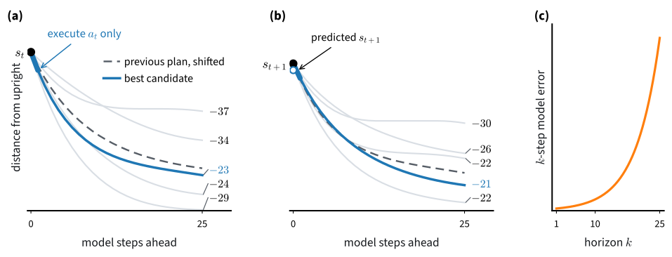
mpc builds such a controller from a model. The plans live in the controller’s closure, one per environment, created at its first call; the perturbation has standard deviation equal to the torque bound, \(c = 2\). In separate runs with five seeds, scored on another set of ten starts, we compared it with a planner that draws 500 fresh, uniformly random sequences at every step. After 600 real steps the warm-started planner scored between about \(-115\) and \(-155\) on every run, and the fresh planner between about \(-165\) and \(-555\); after 1,000 real steps the fresh planner was still 40 to 110 points worse on every seed.
def mpc(model, rng, horizon=horizon, noise=c):
    """Model-predictive control: at every step plan in the model, starting
    from the previous plan shifted by one step, and execute its first
    action."""
    plans = None
    def controller(obs):
        nonlocal plans
        if plans is None:
            plans = np.zeros((len(obs), horizon, 1), np.float32)
        shifted = np.concatenate([plans[:, 1:], np.zeros_like(plans[:, :1])],
                                 1)
        plans = plan(model, obs, shifted, rng, noise)[0]
        return plans[:, 0]
    return controller
def mpc(model, rng, horizon=horizon, noise=c):
"""Model-predictive control: at every step plan in the model, starting
from the previous plan shifted by one step, and execute its first
action."""
plans = None
def controller(obs):
nonlocal plans
if plans is None:
plans = np.zeros((len(obs), horizon, 1), np.float32)
shifted = np.concatenate([plans[:, 1:], np.zeros_like(plans[:, :1])],
1)
plans = plan(model, obs, shifted, rng, noise)[0]
return plans[:, 0]
return controller15.6.2.3 Swing-Up from a Few Episodes
How many real steps does the planner need? mpc_run starts with one random episode. Then, three times, it refits the model on all data so far, scores the planner on the ten test starts, and runs one episode with the planner to collect more data; a last refit and score follow. The scores therefore measure the planner built from 200, 400, 600 and 800 real steps.
def mpc_run(seed, num_rounds=3):
    """One random episode, then rounds of: refit the model on all data,
    score the planner on the ten test starts, collect one MPC episode."""
    env = gym.make_vec('Pendulum-v1', num_envs=1, vectorization_mode='sync')
    rng, (model, opt) = np.random.default_rng(seed), make_model(seed)
    buffer = d2l.ReplayBufferC(200 * (num_rounds + 1), 3, 1)
    run_episode(env, random_controller(rng), buffer, seed=seed)
    scores = []
    for r in range(num_rounds + 1):
        fit_model(model, opt, buffer, rng)
        scores.append(score(mpc(model, rng)))
        if r < num_rounds:
            run_episode(env, mpc(model, rng), buffer)
    return scores, buffer
def mpc_run(seed, num_rounds=3):
"""One random episode, then rounds of: refit the model on all data,
score the planner on the ten test starts, collect one MPC episode."""
env = gym.make_vec('Pendulum-v1', num_envs=1, vectorization_mode='sync')
rng, (model, opt) = np.random.default_rng(seed), make_model(seed)
buffer = d2l.ReplayBufferC(200 * (num_rounds + 1), 3, 1)
run_episode(env, random_controller(rng), buffer, seed=seed)
scores = []
for r in range(num_rounds + 1):
fit_model(model, opt, buffer, rng)
scores.append(score(mpc(model, rng)))
if r < num_rounds:
run_episode(env, mpc(model, rng), buffer)
return scores, bufferThe printout shows the returns of the four collected episodes and the four scores, for five seeds:
runs = [mpc_run(seed) for seed in range(num_seeds)]
print('seed  episode returns: random, MPC x 3 |'
      '  test score at 200/400/600/800 steps')
for seed, (scores, buf) in enumerate(runs):
    rets = buf.rew[:buf.size].reshape(-1, 200).sum(1)
    print(f'{seed:4d} ' + ''.join(f'{r:7.0f}' for r in rets) + '  | '
          + ''.join(f'{s:7.0f}' for s in scores))
seed episode returns: random, MPC x 3 | test score at 200/400/600/800 steps
0 -1072 -242 -118 -125 | -181 -168 -168 -171
1 -876 -264 -121 -123 | -266 -201 -204 -180
2 -966 -122 -125 -116 | -337 -190 -168 -169
3 -1501 -1287 -246 -2 | -1464 -265 -191 -195
4 -1703 -1576 -1323 -120 | -1567 -1437 -171 -187runs = [mpc_run(seed) for seed in range(num_seeds)]
print('seed episode returns: random, MPC x 3 |'
' test score at 200/400/600/800 steps')
for seed, (scores, buf) in enumerate(runs):
rets = buf.rew[:buf.size].reshape(-1, 200).sum(1)
print(f'{seed:4d} ' + ''.join(f'{r:7.0f}' for r in rets) + ' | '
+ ''.join(f'{s:7.0f}' for s in scores))seed episode returns: random, MPC x 3 | test score at 200/400/600/800 steps
0 -1072 -236 -119 -125 | -174 -169 -166 -170
1 -876 -267 -120 -123 | -215 -192 -214 -179
2 -966 -124 -125 -116 | -179 -182 -205 -169
3 -1501 -1541 -1273 -2 | -1550 -1393 -178 -170
4 -1703 -1471 -936 -125 | -1512 -649 -171 -175What is a good score? From the ten test starts, a controller that swings up and balances loses close to nothing from the start nearest the top and about 250 to 320 from each of the five starts near the bottom, about 170 on average. The soft actor-critic of Section 15.5, its greedy actor scored the same way after every episode, settles near \(-170\) and first reaches \(-200\) after about 5,000 to 7,500 steps at one update per step.
After 600 real steps, three episodes, the planner scores between about \(-165\) and \(-215\) on every run, close to that level, and after 800 steps between about \(-170\) and \(-195\). It first reaches \(-200\) after 200 to 800 real steps, and by 600 on all runs but one. On three of the five seeds the model of the random episode alone already gives a planner that scores between about \(-175\) and \(-340\), far from the random policy’s \(-1{,}000\) and below. On the other two, seeds 3 and 4, the first planner fails, with a score near \(-1{,}500\); its first one or two episodes fail as well, and after 600 real steps the same planner succeeds.
15.6.2.4 Coverage
The two slow seeds are the two whose random episode lost the most, about \(1{,}500\) and \(1{,}700\): the random torques never lifted the pendulum above the horizontal. We take the model fitted to that one random episode for each seed, as in the error table above, and test it along the planner’s own episodes instead of a second random one:
print('seed   k=1    k=5   k=10   k=25   (degrees, the planner\'s episodes)')
for seed, ((m, _), (_, buf)) in enumerate(zip(models, runs)):
    errors = kstep_error(m, buf, first=200)      # skip the random episode
    print(f'{seed:4d} ' + ' '.join(f'{e:6.1f}' for e in errors))
seed k=1 k=5 k=10 k=25 (degrees, the planner's episodes)
0 0.3 1.4 3.3 42.4
1 0.4 1.5 2.6 40.2
2 0.2 0.9 1.7 28.3
3 6.8 41.3 61.5 138.8
4 14.8 71.9 89.8 128.3print('seed k=1 k=5 k=10 k=25 (degrees, the planner\'s episodes)')
for seed, ((m, _), (_, buf)) in enumerate(zip(models, runs)):
errors = kstep_error(m, buf, first=200) # skip the random episode
print(f'{seed:4d} ' + ' '.join(f'{e:6.1f}' for e in errors))seed k=1 k=5 k=10 k=25 (degrees, the planner's episodes)
0 0.2 1.0 3.2 56.4
1 0.3 0.9 1.8 27.7
2 0.2 0.9 1.8 29.3
3 7.9 48.5 81.8 120.3
4 10.8 56.4 78.5 87.5On seeds 0 to 2 the errors along the planner’s episodes start as small as on random data, a fraction of a degree after one step, and grow to tens of degrees after 25 steps. These episodes spend most of their time near the upright position, where the pendulum is unstable and a small error in the predicted angle decides on which side it falls. On seeds 3 and 4 the error is several degrees after a single step and tens of degrees after five. The model is accurate where its data went and wrong elsewhere. On the lake, a pair that had never been tried looked worthless to the counted model; here the network extrapolates into the upper half circle it has never seen, and its extrapolation is wrong. The planner’s failed attempts are what repair it: an attempt to swing up, even a failed one, carries the pendulum higher than random torques did and records what happens there. On the next refit the model has data from those states, and the plan built on it works. The planner explores without any explicit exploration rule, because it goes where the model promises reward and the model is corrected wherever it was wrong.
15.6.2.5 The Cost of a Real Step
The planner first reaches \(-200\) after 200 to 800 real steps. On the same score, the mean over the ten test starts, soft actor-critic first reaches \(-200\) after about 5,000 to 7,500 real steps at one gradient step per environment step, and after about 1,600 to 4,000 at ten gradient steps per environment step. These are runs of the code of Section 15.5, with its learned temperature, five seeds per setting, and the counts include its first thousand steps of random warm-up. On the axis of environment steps the planner needs about ten times fewer than the first and a few times fewer than the second.
The other axis is computation. Every action of the planner is a search: 12,500 evaluations of the model, a few milliseconds on one CPU core for this small network, and every episode adds a refit of a thousand Adam steps. Soft actor-critic takes one or ten gradient steps of three small networks per real step, and acting needs only one forward pass of its actor. A real robot must also finish the search within its control period, here 0.05 seconds. The model does not make learning free. It moves the cost from experience, which is scarce on a robot, to computation, which is scarce on the robot’s controller.
15.6.3 Search as Policy Improvement
15.6.3.1 Search Seeded by the Actor
The planner has no policy. Every action requires a full search, and nothing it finds is remembered except through the model and the shifted plan of the last step. A policy network would act with one forward pass and generalize across states, but it must be trained, and Section 15.5 needed thousands of steps to train one through a critic. Can the search train the policy instead?
Start the search from the policy’s own plan. Let the actor be a network that maps a state to a torque, \(\bar a_\theta(s)\). In the model, the actor’s plan from state \(s\) is the sequence of torques it chooses along its own predicted trajectory: \(a_0 = \bar a_\theta(s)\), \(\hat s_1\) from \(\hat f_\phi(s, a_0)\), \(a_1 = \bar a_\theta(\hat s_1)\), and so on for \(n\) steps. actor_plan computes it for a batch of states. improve hands this plan to plan in place of the shifted previous plan, with the same 500 candidates and the same perturbation, and returns the first torque of the best candidate.
def actor_plan(model, actor, obs, horizon=horizon):
    """The actor's own deterministic plan for each state, imagined in the
    model: (B, n, 1)."""
    acts = []
    for _ in range(horizon):
        acts.append(actor.act_greedy(obs))
        obs = np.asarray(rollout_model(model, obs, acts[-1][:, None])[0])[:, 0]
    return np.stack(acts, 1)

def improve(model, actor, obs, rng, noise=c):
    """Search seeded by the actor: the best first action for each state."""
    return plan(model, obs, actor_plan(model, actor, obs), rng, noise)[0][:, 0]
def actor_plan(model, actor, obs, horizon=horizon):
"""The actor's own deterministic plan for each state, imagined in the
model: (B, n, 1)."""
acts = []
for _ in range(horizon):
acts.append(actor.act_greedy(obs))
obs = np.asarray(rollout_model(model, obs, acts[-1][:, None])[0])[:, 0]
return np.stack(acts, 1)
def improve(model, actor, obs, rng, noise=c):
"""Search seeded by the actor: the best first action for each state."""
return plan(model, obs, actor_plan(model, actor, obs), rng, noise)[0][:, 0]Since the actor’s own plan is one of the candidates, the search returns an action whose plan has a predicted return at least as high as the actor’s plan. Under the model and over \(n\) steps, search seeded by a policy is never worse than the policy. This is the greedy step of policy iteration in Section 14.2.3.2, which chose at every state an action at least as good as the current policy’s, judged by the policy’s own values; here the judge is the model’s prediction over the next 25 steps. The guarantee holds only inside the model and only over the horizon. A wrong model can certify a worse action, and a plan that ends after 25 steps cannot value what happens later.
15.6.3.2 Distillation into the Actor
If the search improves on the actor, we can train the actor to imitate the search. This is the behavior cloning of Section 14.5 with the search as the expert: label states with improve and regress the actor’s torque onto the labels with a squared error, since the torque is continuous. The actor is d2l.SquashedGaussianPolicy from Section 15.5, a two-layer network whose Gaussian mean is squashed by \(c \tanh\) into the torque range; we train only its squashed mean \(\bar a_\theta(s) = c \tanh \mu_\theta(s)\), with \(\mu_\theta\) the Gaussian mean as there, which is what its act_greedy returns. make_actor builds the actor with its Adam optimizer, and distill takes 1,000 Adam steps of this regression.
def make_actor(seed, lr=1e-3):
    torch.manual_seed(seed)
    actor = d2l.SquashedGaussianPolicy(3, 1, scale=c)
    return actor, torch.optim.Adam(actor.parameters(), lr=lr)

def distill(actor, opt, obs, labels, rng, num_steps=1_000, batch_size=256):
    """Regress the actor's mean action, scale * tanh(mean), onto labels."""
    obs, labels = torch.as_tensor(obs), torch.as_tensor(labels)
    for _ in range(num_steps):
        i = torch.as_tensor(rng.integers(len(obs), size=batch_size))
        a = actor.scale * torch.tanh(actor.policy(obs[i])[0])
        loss = ((a - labels[i]) ** 2).mean()
        opt.zero_grad()
        loss.backward()
        opt.step()
    return float(loss.detach())
def make_actor(seed, lr=1e-3):
actor = d2l.SquashedGaussianPolicy(3, 1, scale=c, rngs=nnx.Rngs(seed))
return actor, nnx.Optimizer(actor, optax.adam(lr), wrt=nnx.Param)
@nnx.jit
def distill_step(actor, opt, obs, labels):
loss = lambda m: ((m.scale * jnp.tanh(m.policy(obs)[0]) - labels)
** 2).mean()
value, grads = nnx.value_and_grad(loss)(actor)
opt.update(actor, grads)
return value
def distill(actor, opt, obs, labels, rng, num_steps=1_000, batch_size=256):
"""Regress the actor's mean action, scale * tanh(mean), onto labels."""
step = nnx.cached_partial(distill_step, actor, opt)
for _ in range(num_steps):
i = rng.integers(len(obs), size=batch_size)
loss = step(obs[i], labels[i])
return float(loss)distill_step is one compiled Adam step of the regression, bound to the actor and its optimizer once per call of distill by nnx.cached_partial, as model_step was bound to the model.
Each round of search_and_distill refits the model, labels 200 stored states drawn at random with the search, distills these labels into the actor, and collects one real episode acting with search. Only the current round’s labels train the actor; the labels of earlier rounds are not kept. Acting with search makes each episode as good as the current model and actor allow, so the data reach the states a good controller visits. With a network that also predicts the value of each state, a tree search over discrete moves, and a buffer that keeps the search’s targets over many games, this loop of acting with search, labeling and distilling is the loop of AlphaZero.
The loop records per round the return of the episode collected with search and the score of the actor alone, acting with no search at all; at the end it scores acting with search on the ten starts. The two curves measure different things. The first is one training episode per round, from wherever that episode happens to start, so it moves with the start state as much as with the agent; a single hard start shows up as a dip. The second is the mean over the ten test starts, the score used everywhere else in this section.
def search_and_distill(seed, num_rounds=8, num_labels=200):
    """One random episode, then rounds of: refit the model, label stored
    states with the search, regress the actor onto the labels, collect one
    episode acting with search. Returns per round the collected return and
    the actor's score alone, and the final score acting with search."""
    env = gym.make_vec('Pendulum-v1', num_envs=1, vectorization_mode='sync')
    rng, (model, opt) = np.random.default_rng(seed), make_model(seed)
    actor, actor_opt = make_actor(seed)
    buffer = d2l.ReplayBufferC(200 * (num_rounds + 1), 3, 1)
    run_episode(env, random_controller(rng), buffer, seed=seed)
    search = lambda obs: improve(model, actor, obs, rng)
    rounds = []
    for _ in range(num_rounds):
        fit_model(model, opt, buffer, rng)
        obs = buffer.obs[rng.choice(buffer.size, num_labels, replace=False)]
        distill(actor, actor_opt, obs, search(obs), rng)
        rounds.append([run_episode(env, search, buffer)[0],
                       score(actor.act_greedy)])
    return np.array(rounds), score(search)
def search_and_distill(seed, num_rounds=8, num_labels=200):
"""One random episode, then rounds of: refit the model, label stored
states with the search, regress the actor onto the labels, collect one
episode acting with search. Returns per round the collected return and
the actor's score alone, and the final score acting with search."""
env = gym.make_vec('Pendulum-v1', num_envs=1, vectorization_mode='sync')
rng, (model, opt) = np.random.default_rng(seed), make_model(seed)
actor, actor_opt = make_actor(seed)
buffer = d2l.ReplayBufferC(200 * (num_rounds + 1), 3, 1)
run_episode(env, random_controller(rng), buffer, seed=seed)
search = lambda obs: improve(model, actor, obs, rng)
rounds = []
for _ in range(num_rounds):
fit_model(model, opt, buffer, rng)
obs = buffer.obs[rng.choice(buffer.size, num_labels, replace=False)]
distill(actor, actor_opt, obs, search(obs), rng)
rounds.append([run_episode(env, search, buffer)[0],
score(actor.act_greedy)])
return np.array(rounds), score(search)Eight rounds start from one random episode, so the actor of round \(r\) has seen \(200 r\) real steps. We run three seeds and plot the median with the range over seeds:
results = [search_and_distill(seed) for seed in range(3)]
rounds = np.array([r for r, _ in results])
d2l.plot_curves({'episode acting with search': rounds[:, :, 0],
                 'actor alone, ten starts': rounds[:, :, 1]},
                'real environment steps', 'return',
                x=200 * np.arange(1, 9), reference=-200)
print('final score on the ten starts, acting with search:',
      ' '.join(f'{s:.0f}' for _, s in results))
final score on the ten starts, acting with search: -191 -202 -222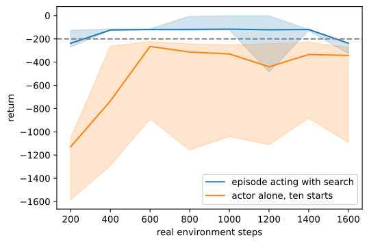
results = [search_and_distill(seed) for seed in range(3)]
rounds = np.array([r for r, _ in results])
d2l.plot_curves({'episode acting with search': rounds[:, :, 0],
                 'actor alone, ten starts': rounds[:, :, 1]},
                'real environment steps', 'return',
                x=200 * np.arange(1, 9), reference=-200)
print('final score on the ten starts, acting with search:',
      ' '.join(f'{s:.0f}' for _, s in results))
final score on the ten starts, acting with search: -199 -319 -185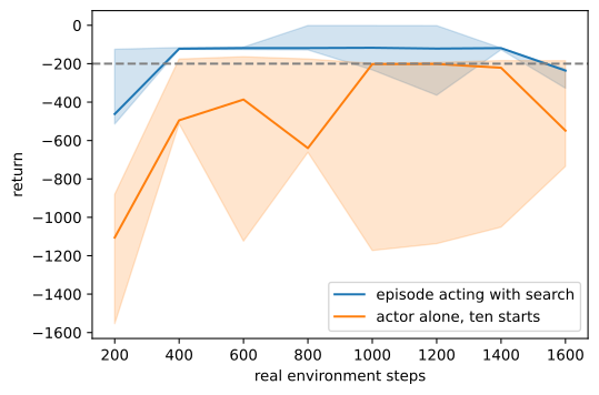
15.6.3.3 Rounds of Search and Distillation
Acting with search, the agent swings the pendulum up within two or three rounds on each of the three runs shown, and after eight rounds it scores between about \(-185\) and \(-320\) on the ten starts, close to the warm-started planner above on most runs. The actor alone improves on every run, from between about \(-900\) and \(-1{,}600\) after the first round to between about \(-190\) and \(-1{,}100\) after the eighth, and its score can drop by hundreds from one round to the next. The network has learned part of what the search knows; acting on its own, it falls short.
These runs do not show why it falls short, and three causes are candidates. The first is the distribution shift that Section 14.5 measured on the lake. The labels are drawn from the stored states, and apart from the random episode these are states the search visited. An actor that imitates the search imperfectly drifts, when it acts alone, into states with few labels, and its errors compound there. DAgger (Section 14.5.4.1) repaired this on the lake by labeling the learner’s own states. The second is the size of the training set: each round trains the actor on 200 fresh labels and discards the earlier ones, while DAgger aggregates its labels over all rounds and AlphaZero keeps its search targets in a buffer. The third is the labels themselves: each is the first torque of the best of 500 random candidates, a noisy target. Exercise 5 separates the first two causes. AlphaZero also searches at test time, so its network only has to make the search’s starting point good. The search and the network then improve each other: a better actor seeds a better search, and a better search teaches the actor.
15.6.3.4 Imagined Transitions as Data
A model can also feed a learner that has no planner. Dyna (Sutton 1990) interleaves real steps with updates on transitions sampled from the model, and model-based policy optimization (MBPO) (Janner et al. 2019) does this for soft actor-critic: every few hundred steps it refits the model, rolls the current actor out in the model for a few steps from states in the replay buffer, and fills most of each training batch with these imagined transitions. The imagined data are as plentiful as computation allows. The model’s errors, however, enter the critic’s targets, and short rollouts are how MBPO limits the compounding error measured above.
Does this reduce the real steps on Pendulum? We ran soft actor-critic with its temperature fixed at 0.2, ten gradient steps per environment step, and batches made of 5% real and 95% imagined transitions from three-step rollouts, refitting the model every 250 steps. Over five seeds its greedy actor first scored \(-200\) or better after 1,500 to 3,000 steps; without the model, at the same ten updates per step, it took 1,500 to 2,500. These runs used another set of ten fixed starts, from which a good controller loses less than from ours, so they reach \(-200\) sooner than the runs quoted above. At a matched update ratio the imagined transitions did not reduce the real steps. Much of what MBPO gains over soft actor-critic at one update per step can come from the extra updates per real step, which replay supplies without a model; a model-free learner with a high update ratio and an ensemble of critics to control the overestimation that such ratios cause matched MBPO’s sample efficiency (Chen et al. 2021). Exercise 6 repeats the comparison. A model helps most where this section used it: to look ahead before acting and to turn the search into a policy. Ensembles of models that know where they are uncertain, models of a learned latent state, and searches that end in a learned value carry these ideas further; Section 15.9 describes them.
We can now fit a model of the dynamics from a few hundred steps, plan through it, and teach a policy what the search finds. Every step trusted the model only where its own episodes had gone and only for 25 steps, and it could test that trust by acting and refitting. Section 15.7 takes away the acting: the data are a fixed log, and nothing that a model or a value function promises beyond that log can be checked.
15.6.4 Summary
A transition records how the environment moves, and a network fitted to transitions by least squares, \(\hat f_\phi(s, a) \to (\hat s', \hat r)\), extends the counted model of the lake to continuous states. Its one-step errors are small, but they compound along a rollout, and they are large wherever the data never went. Model-predictive control searches torque sequences in the model, executes the first torque and plans again at the next step; with a warm start, a planner built from one to three episodes swings the pendulum up after a few hundred real steps, where soft actor-critic needed thousands, and each of its actions needs thousands of model evaluations. A search seeded by a policy never predicts a lower return than the policy, so it improves the policy, and regressing the actor onto the search’s actions transfers part of that improvement; acting alone, the actor lags behind. Its labels lie mostly on the search’s states, are few per round, and are noisy, and these runs do not say which of the three matters most. Imagined transitions as training data did not reduce the real steps of soft actor-critic at a matched number of updates per step.
15.6.5 Exercises
- [code] Depth of the plan. The planner looks \(n = 25\) steps ahead.
- Before running anything, use the two error tables of this section to predict what happens to the test score with \(n = 10\) and with \(n = 50\), keeping 500 candidates.
- Run
mpc_runwith both depths for three seeds and compare the scores after 600 real steps with those for \(n = 25\). - A swing-up from the bottom takes a few dozen steps of pumping. Explain the result for \(n = 10\) by what its predicted returns can and cannot distinguish, and the result for \(n = 50\) by the error tables. How does the cost of one action change with \(n\)?
- [code] How much random data. Seeds 3 and 4 needed the planner’s own failed episodes before the model covered the upper half circle.
- For both seeds, fit the model to one, two and five random episodes. Report the highest point the pendulum reached in the data (the largest \(\cos\vartheta\)) and the 25-step error of each model along the planner’s episodes, as in the coverage table.
- How many random episodes does a planner built from random data alone need to swing up from most test starts? Compare with the 600 steps that the planner’s own episodes needed, and explain the difference.
- [code] The cross-entropy method. The cross-entropy method (Rubinstein and Kroese 2004) repeats random shooting several times per action and refits the sampling distribution to the best candidates.
- Change
planso that it runs five rounds: after each, set the mean and the standard deviation of every torque of the plan to those of the 50 best of the 500 candidates, and draw the next 500 from this Gaussian. - Compare the test scores after 600 real steps and the model evaluations per action with the warm-started random shooting of this section.
- Run the method without the warm start, starting every step from a mean of zero torque and a standard deviation of \(c\). Does refining within one step replace refining across steps?
- Change
- [code] Disagreement as a trust signal. ● An ensemble of models can say where it does not know (Chua et al. 2018).
- For seeds 3 and 4, fit three models with different seeds to the random episode. Along the planner’s episodes, compare the disagreement of the three models (the standard deviation of their predicted angles) with the error of their mean prediction after 1, 5 and 25 steps. Does a large disagreement predict a large error?
- Score each candidate in
planby the mean predicted return of the three models minus \(\kappa\) times the disagreement summed over its steps, for \(\kappa \in \{0, 1, 10\}\). How does the first MPC episode of seeds 3 and 4 change? - Repeat part b with \(-\kappa\), a bonus for disagreement. Which sign suits an agent that can still collect data, and which an agent that cannot?
- [code] Labels on the actor’s own states. ● The loop of this section collects its episodes acting with search and trains the actor each round only on that round’s 200 labels.
- Keep collecting with search, but aggregate the labels: append each round’s labeled states and torques to one growing set and distill the actor on the whole set. Run five seeds and compare the actor’s scores per round with those of this section.
- Now collect every round’s episode with the actor alone,
actor.act_greedy, label states of the actor’s episodes withimprove, and aggregate the labels as in part (a). This is DAgger of Section 14.5, with the search as the expert. Which of the three versions gives the steadier actor, and what does the comparison say about the causes named in the text? - On some seeds the DAgger version may never swing the pendulum up. Inspect the data of such a run and explain the failure with the coverage table of this section. How could the two ways of collecting data be combined?
- [extended] Imagined transitions for soft actor-critic. ●● Model-based policy optimization (Janner et al. 2019) trains soft actor-critic on transitions imagined by a model.
- Copy
train_sacfrom Section 15.5 into your notebook. After the warm-up, every 250 environment steps, refit aDynamicsModelon the replay buffer and roll the current actor out for three steps in the model from 2,000 states drawn from the buffer. Keep the imagined transitions of the last four refits in a secondd2l.ReplayBufferCand draw 95% of every batch from it. - With ten updates per environment step, run five seeds for 4,000 steps, and score the greedy actor on the ten test starts every 250 steps. Run the control arm, the same loop without the model, with the same seeds. Report the first step at which each run scores \(-200\) or better.
- Why must the control arm use the same number of updates per environment step? Repeat both arms with one update per step and interpret the difference.
- Change the rollout length to one step and to ten steps. Which result does the error table of this section predict, and what do you observe?
- Copy
- [code] Lookahead with a value. The planner of this section adds rewards over a fixed horizon and ignores what comes after it. With a value function the horizon can be one step.
- On CartPole, fit a
DynamicsModelwith a four-dimensional state to 5,000 transitions of random actions; let the pole’s angle and the cart’s position decide termination by CartPole’s known rule. - Train the DQN of Section 15.4 for 10,000 steps and act greedily in two ways: by \(\operatorname{argmax}_a Q(s, a)\), and by the one-step lookahead \(\operatorname{argmax}_a \big[\hat r(s, a) + \gamma \max_{a'} Q(\hat s'(s, a), a')\big]\). Compare the returns over 20 episodes for five seeds.
- Repeat after 40,000 steps of training. When does the lookahead help, and when do the model’s errors outweigh what it adds?
- On CartPole, fit a