from d2l import torch as d2l
import math
import numpy as np
import torch27.3 The Exponential Family
The previous section built its catalogue of distributions one law at a time: a coin, the number of heads in many flips, rare events, waiting times, the bell curve. Each law came with its own formula, and each mean and variance needed its own trick. The models of the main text show a similar pattern. Linear regression, logistic regression and softmax regression each come with a loss of their own. Yet when we differentiate these losses, all three give the same training rule: the input times the difference between the prediction and the observation. Agreement of this kind usually has a single cause.
Take the coin that runs through this chapter, which came up heads 9 times in 13 flips. The obvious estimate of its bias is \(9/13\approx0.69\). A logistic-regression model with only a bias term, fitted to the same flips, reaches this number by a detour: its last layer computes the log-odds \(\log(9/4)\approx0.81\), and a sigmoid turns that into \(9/13\). Why does a classifier work with the log-odds rather than with the probability itself?
Both observations have one explanation. Nearly every distribution of the catalogue can be written in a common form, in which the parameters act through the exponential of a linear function of a few statistics of the data. Distributions of this form make up the exponential family, and for the coin the parameter in the exponent is the log-odds. Four facts follow from the form alone. The mean and the variance are the first two derivatives of one function. Fitting by maximum likelihood is a convex problem whose gradient is prediction minus observation. The softmax is what the form gives for class labels. And a prior of the same form is updated by adding counts.
These facts help whenever a new kind of label comes along, such as a count or a waiting time. The form tells us which loss to train with and guarantees that fitting a linear model to it is a convex problem. It also shows when the fit has no solution at all, as for a coin that came up heads in every flip. We start from the catalogue of Section 27.2 and end with a question this section leaves open: how far can the estimate \(9/13\) be from the true bias of the coin?
The shared computations of this section use NumPy; each framework’s automatic differentiation computes the derivatives of the log-partition function.
from d2l import tensorflow as d2l
import math
import numpy as np
import tensorflow as tf
from d2l import jax as d2l
import jax
import jax.numpy as jnp
import math
import numpy as npfrom d2l import mxnet as d2l
from mxnet import autograd, nd
import math
import numpy as np27.3.1 One Form for Many Distributions
We begin with the smallest distribution of the catalogue, a single coin flip, and rewrite it until the log-odds appears. The rewriting shows what the general form has to look like.
27.3.1.1 The Bernoulli in Exponential Form
A coin with bias \(p\) shows heads (\(x=1\)) with probability \(p\) and tails (\(x=0\)) with probability \(1-p\), which the previous section wrote compactly as \(p^x(1-p)^{1-x}\). To see how the outcome \(x\) and the parameter \(p\) interact, we take the logarithm and collect the terms that contain \(x\):
\[ \log P(X=x) = x\log p + (1-x)\log(1-p) = x\log\frac{p}{1-p} + \log(1-p). \]
The outcome enters only through \(x\) itself, multiplied by the log-odds \(\log\frac{p}{1-p}\), and the remaining term depends on \(p\) alone. We name the log-odds \(\eta=\log\frac{p}{1-p}\) and express the second term through it. Solving for \(p\) gives \(p=e^\eta/(1+e^\eta)\), so \(1-p=1/(1+e^\eta)\) and \(\log(1-p)=-\log(1+e^\eta)\). Exponentiating,
\[ P(X=x) = \exp\bigl(x\eta - \log(1+e^\eta)\bigr), \qquad x\in\{0,1\}. \]
The coin’s probability is the exponential of a linear function of \(x\) minus a term that does not involve \(x\). That term is the normalizer: the two unnormalized probabilities are \(e^{0}=1\) and \(e^\eta\), and they sum to \(1+e^\eta\).
Three pieces of this formula will recur. The statistic \(T(x)=x\) is what the outcome contributes. The natural parameter \(\eta\) multiplies it; for the coin it is the log-odds, also called the logit. The log-partition function \(A(\eta)=\log(1+e^\eta)\) is the logarithm of the normalizer, a function known as the softplus. Reading the substitution backward,
\[ p = \frac{e^\eta}{1+e^\eta} = \operatorname{sigmoid}(\eta), \qquad \operatorname{sigmoid}(\eta)=\frac{1}{1+e^{-\eta}}. \]
The sigmoid of logistic regression is therefore the map from the coin’s natural parameter back to its mean, and it follows from the Bernoulli itself.
For the chapter’s coin, the estimate \(9/13\) corresponds to the natural parameter
\[ \hat\eta = \log\frac{9/13}{4/13} = \log\frac94 \approx 0.811, \]
and the sigmoid maps it back, \(\operatorname{sigmoid}(\log\frac94)=\frac{9/4}{1+9/4}=\frac{9}{13}\). We show below that \(\hat\eta\) is the maximum-likelihood value of the log-odds, and we ask what the curvature of the loss at \(\hat\eta\) tells us.
27.3.1.2 Definition and Members
The coin’s rewriting has three parts: a statistic of the data, a parameter that multiplies it, and a normalizer. Allowing several statistics at once, and a fixed weight on each outcome, gives a form that fits most of the catalogue.
A family of distributions is an exponential family if its probability mass or density function can be written as
\[ p(\mathbf x\mid\boldsymbol\eta) = h(\mathbf x)\,\exp\bigl(\boldsymbol\eta^\top T(\mathbf x) - A(\boldsymbol\eta)\bigr). \tag{27.3.1}\]
The data and the parameters meet only in the inner product \(\boldsymbol\eta^\top T(\mathbf x)\). The base measure \(h(\mathbf x)\ge0\) is a fixed weight on the outcomes that does not depend on the parameters; the set where \(h>0\) is the support. The natural parameters \(\boldsymbol\eta\in\mathbb R^d\) are the adjustable parameters, and the sufficient statistics \(T(\mathbf x)\in\mathbb R^d\) are the features of the data that they multiply. The log-partition function is the logarithm of the normalizer,
\[ A(\boldsymbol\eta) = \log\int h(\mathbf x)\,\exp\bigl(\boldsymbol\eta^\top T(\mathbf x)\bigr)\,d\mathbf x, \tag{27.3.2}\]
with a sum in place of the integral for discrete \(\mathbf x\). Thus \(A\) is whatever makes Equation 27.3.1 sum or integrate to one, and the natural parameters range over the set where \(A(\boldsymbol\eta)\) is finite. The coin is the case \(h(x)=1\), \(T(x)=x\) and \(A(\eta)=\log(1+e^\eta)\).
The name sufficient says what \(T\) does for estimation. For \(n\) independent observations the likelihood is
\[ \prod_{i=1}^n p(\mathbf x_i\mid\boldsymbol\eta) = \Bigl(\prod_{i=1}^n h(\mathbf x_i)\Bigr) \exp\Bigl(\boldsymbol\eta^\top\sum_{i=1}^n T(\mathbf x_i) - nA(\boldsymbol\eta)\Bigr), \]
so the parameters touch the data only through the sum \(\sum_i T(\mathbf x_i)\). Two data sets with the same sum have likelihoods that differ by a factor that does not depend on \(\boldsymbol\eta\), and they lead to the same estimates. For the coin the sum is the number of heads, so the order of the 13 flips is irrelevant. The base measure does depend on \(\mathbf x\), so \(T(\mathbf x)\) does not fix the probability of \(\mathbf x\); it fixes everything in \(\mathbf x\) that carries information about \(\boldsymbol\eta\).
Matching the pieces identifies the other members. The Poisson probability of \(k\) events at rate \(\lambda\) is \(\frac{\lambda^ke^{-\lambda}}{k!}=\frac1{k!}\exp(k\log\lambda-\lambda)\), so \(h(k)=1/k!\), \(T(k)=k\), \(\eta=\log\lambda\) and \(A(\eta)=e^\eta=\lambda\). The Gaussian with unknown mean and variance needs two statistics. Expanding the square in its exponent and collecting the terms in \(x\) and in \(x^2\) gives
\[ \frac{1}{\sqrt{2\pi}}\exp\Bigl(\underbrace{\tfrac{\mu}{\sigma^2}}_{\eta_1}\,x + \underbrace{\bigl(-\tfrac{1}{2\sigma^2}\bigr)}_{\eta_2}\,x^2 - \underbrace{\bigl(\tfrac{\mu^2}{2\sigma^2}+\log\sigma\bigr)}_{A(\boldsymbol\eta)}\Bigr), \]
so \(T(x)=(x,x^2)^\top\) and \(h(x)=1/\sqrt{2\pi}\). The second natural parameter must be negative: with \(\eta_2<0\) the factor \(e^{\eta_2x^2}\) produces the Gaussian’s decay, and with \(\eta_2\ge0\) the integral that defines \(A\) diverges. Table 27.3.1 lists these and other members.
| distribution | \(h(\mathbf x)\) | \(T(\mathbf x)\) | \(\boldsymbol\eta\) | \(A(\boldsymbol\eta)\) |
|---|---|---|---|---|
| Bernoulli(\(p\)) | \(1\) | \(x\) | \(\log\frac{p}{1-p}\) | \(\log(1+e^\eta)\) |
| Binomial(\(n,p\)) | \(\binom nx\) | \(x\) | \(\log\frac{p}{1-p}\) | \(n\log(1+e^\eta)\) |
| Poisson(\(\lambda\)) | \(1/k!\) | \(k\) | \(\log\lambda\) | \(e^\eta\) |
| Categorical, one-hot \(\mathbf y\) | \(1\) | \(\mathbf y\) | logits \(\mathbf z\) | \(\log\sum_k e^{z_k}\) |
| Exponential(\(\lambda\)) | \(1\) for \(x\ge0\) | \(x\) | \(-\lambda\) | \(-\log(-\eta)\) |
| \(\mathcal N(\mu,\sigma^2)\) | \(1/\sqrt{2\pi}\) | \((x,x^2)\) | \(\bigl(\frac{\mu}{\sigma^2},-\frac{1}{2\sigma^2}\bigr)\) | \(-\frac{\eta_1^2}{4\eta_2}-\frac12\log(-2\eta_2)\) |
| Laplace(\(\mu,b\)) | \(1\) | \(\lvert x-\mu\rvert\) | \(-1/b\) | \(\log(-2/\eta)\) |
The categorical row writes the class probabilities through the logits. They form the softmax, whose origins Section 27.3.4 takes up. Two more members need matrices: the multivariate Gaussian, with the statistics \(\mathbf x\) and \(\mathbf x\mathbf x^\top\) and the natural parameters \(\boldsymbol\Sigma^{-1}\boldsymbol\mu\) and \(-\frac12\boldsymbol\Sigma^{-1}\), and the multinomial with a fixed number of draws. The split between \(h\), \(\boldsymbol\eta\) and \(T\) is not unique: scaling \(T\) by a constant and dividing \(\boldsymbol\eta\) by the same constant, for instance, describes the same distribution.
27.3.1.3 Distributions Outside the Family
Not every distribution has this form. Two kinds fall outside it for different reasons, and the first shows which property of the form the later results rely on.
The uniform distribution \(U(0,\theta)\) has the density \(1/\theta\) on \([0,\theta]\) and zero elsewhere, so its support moves with the parameter. Every member of Equation 27.3.1 has the same support for all parameters, the set where \(h>0\), because the exponential factor is never zero. A moving support changes how estimation works. Take three observations, \(0.1\), \(0.2\) and \(0.9\). The likelihood is \(\theta^{-3}\) when \(\theta\ge0.9\) and \(0\) when \(\theta<0.9\), because a smaller \(\theta\) cannot produce the observation \(0.9\), so it is largest at \(\hat\theta=\max_i x_i=0.9\).
Inside the family, maximum likelihood matches the mean of the sufficient statistic to its sample average, as we show below. The same recipe here sets the mean \(\theta/2\) equal to \(\bar x=0.4\) and gives \(\theta=0.8\), a value under which the observation \(0.9\) is impossible. The uniform’s likelihood depends on the data through their maximum, not through a sum, and the tools of this section do not apply to it. Exercise 8 compares the two estimates as the sample grows.
Heavy-tailed laws fall outside for another reason. The Student-\(t\) distribution is a Gaussian whose precision \(1/\sigma^2\) is itself drawn at random; averaging over the precision turns the \(e^{-x^2}\) tails into polynomial ones. With unit scale and \(\nu\) degrees of freedom, its likelihood for \(n\) observations is a product of the factors \(\bigl(1+(x_i-\mu)^2/\nu\bigr)^{-(\nu+1)/2}\), which no fixed number of sums of the data can summarize.
Two conveniences hold for every exponential family, and we prove both below: a conjugate prior of the same form, and a negative log-likelihood that is convex in the natural parameters. Outside the family they can fail. For the Student-\(t\), the negative log-likelihood of the location \(\mu\) has a separate local minimum near each cluster when the data form two well-separated clusters.
27.3.2 Maximum Entropy
So far the exponential form came from rewriting distributions we already had. A different question explains where it comes from. Suppose that all we know about a random quantity is the average of a few of its statistics: which distribution should we assume? The answer that assumes nothing beyond those averages is a member of the exponential family.
27.3.2.1 Entropy and a Loaded Die
To make “assumes nothing beyond the averages” precise, we need a measure of how spread out a distribution is. For a distribution \(p=(p_1,\dots,p_K)\) on a finite set, the entropy is
\[ H[p] = -\sum_{k=1}^K p_k\log p_k, \]
measured in nats, with the convention \(0\log0=0\). Each term weighs the surprise \(-\log p_k\) of outcome \(k\) by its probability, so the entropy is the average surprise. A fair die has six outcomes of surprise \(\log6\) each and the entropy \(\log6\approx1.79\); a die that always shows a six is never surprising and has entropy \(0\). Among distributions on \(K\) outcomes the uniform one has the largest entropy, \(\log K\), which we prove below.
E. T. Jaynes posed the question in this form (Jaynes 1957). Suppose a die is known to average \(4.5\) rather than \(3.5\), and nothing else is known about it. Many distributions on \(\{1,\dots,6\}\) have this mean. Half threes and half sixes is one, but it asserts that \(1\), \(2\), \(4\) and \(5\) never occur, which nothing we know supports; its entropy is \(\log2\approx0.69\).
Jaynes’ principle picks, among all distributions with the required mean, the one of largest entropy, the least committal choice. We state the answer before proving it. The maximizer is an exponential tilt of the uniform distribution,
\[ p_k = \frac{e^{\eta k}}{\sum_{j=1}^6 e^{\eta j}}, \qquad k=1,\dots,6, \]
with \(\eta\) chosen so that the mean is \(4.5\). How large is \(\eta\), and how much entropy does the constraint remove? The mean of the tilt increases with \(\eta\), so bisection finds the \(\eta\) with mean \(4.5\).
k = np.arange(1, 7)
def tilt(eta):                                   # p_k proportional to exp(eta k)
    w = np.exp(eta * k)
    return w / w.sum()

lo, hi = -5.0, 5.0
for _ in range(50):                              # bisection: the mean increases with eta
    eta = (lo + hi) / 2
    lo, hi = (eta, hi) if (tilt(eta) * k).sum() < 4.5 else (lo, eta)
p = tilt(eta)
print('eta =', round(eta, 3), ' p =', p.round(3))
print('H =', round(-(p * np.log(p)).sum(), 3), ' log 6 =', round(np.log(6), 3))
eta = 0.371 p = [0.054 0.079 0.114 0.165 0.24 0.347]
H = 1.614 log 6 = 1.792The tilt is geometric: each face is \(e^{0.371}\approx1.45\) times as likely as the face below it. The entropy is \(1.61\) nats, \(0.18\) less than that of the fair die, and \(\eta=0\) gives the fair die back. Figure 27.3.1 shows the tilts for three required means.
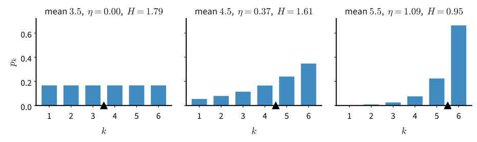
The tilt has the form Equation 27.3.1 with \(h\equiv1\) on the six faces, the statistic \(T(k)=k\) and the natural parameter \(\eta\). Fixing the average of a statistic and maximizing entropy produces the exponential of a multiple of that statistic; the multiple is the natural parameter, and the normalizer is \(e^{A(\eta)}\). The next subsection proves that this holds in general.
27.3.2.2 The Maximum-Entropy Proposition
The general statement needs one extension of entropy, because some sets of outcomes come with natural weights. For a distribution \(q\) and a base measure \(h\), the entropy relative to \(h\) is
\[ H_h[q] = -\sum_{\mathbf x} q(\mathbf x)\log\frac{q(\mathbf x)}{h(\mathbf x)} \]
for discrete outcomes, with an integral for densities. With \(h\equiv1\) it is the entropy defined above. On the counts \(\{0,1,2,\dots\}\), for example, the weights \(h(k)=1/k!\) will lead to the Poisson distribution, while \(h\equiv1\) leads to the geometric distribution.
The proof rests on one inequality, which follows from a tangent line. The logarithm is concave, so its graph lies below its tangent line at \(u=1\): \(\log u\le u-1\) for all \(u>0\), with equality only at \(u=1\).
Lemma (Gibbs’ inequality). Let \(p\) and \(q\) be distributions on the same set such that \(p(\mathbf x)>0\) wherever \(q(\mathbf x)>0\). Then
\[ \sum_{\mathbf x:\,q(\mathbf x)>0} q(\mathbf x)\log\frac{p(\mathbf x)}{q(\mathbf x)} \le 0, \]
with equality only if \(q=p\). For densities, the sums become integrals.
Proof. Apply the tangent-line bound with \(u=p(\mathbf x)/q(\mathbf x)\) and sum over the outcomes with \(q(\mathbf x)>0\):
\[ \sum_{q>0} q\log\frac pq \le \sum_{q>0} q\Bigl(\frac pq-1\Bigr) = \sum_{q>0} p - 1 \le 0. \]
Equality in the first step needs \(p=q\) wherever \(q>0\); then \(\sum_{q>0}p=1\), so \(p\) puts no mass outside the support of \(q\), and \(p=q\). \(\blacksquare\)
The negated left side, \(D_{\textrm{KL}}(q\|p)=\sum q\log(q/p)\), is the Kullback–Leibler divergence of \(q\) from \(p\) (Cover and Thomas 1999), and the lemma says that it is never negative and vanishes only at \(q=p\).
Proposition (maximum entropy). Let \(p(\mathbf x)=h(\mathbf x)\exp(\boldsymbol\eta^\top T(\mathbf x)-A(\boldsymbol\eta))\) be a member of an exponential family, and let \(q\) be any distribution that is zero wherever \(h\) is zero and has the same mean statistic, \(\mathbb{E}_q[T(\mathbf x)]=\mathbb{E}_p[T(\mathbf x)]\). Then \(H_h[q]\le H_h[p]\), with equality only if \(q=p\).
Proof. We split the logarithm in \(H_h[q]\) at \(p\), \(\log\frac qh=\log\frac qp+\log\frac ph\). The first part contributes \(-D_{\textrm{KL}}(q\|p)\le0\) by the lemma, which applies because \(p>0\) wherever \(h>0\). The second part is linear in the statistic, \(\log\frac ph=\boldsymbol\eta^\top T-A(\boldsymbol\eta)\), so only the mean of \(T\) under \(q\) enters:
\[ -\sum_{\mathbf x} q\log\frac ph = -\boldsymbol\eta^\top\mathbb{E}_q[T] + A(\boldsymbol\eta) = -\boldsymbol\eta^\top\mathbb{E}_p[T] + A(\boldsymbol\eta) = H_h[p]. \]
The middle step uses the constraint, and the last step is the same computation with \(p\) in place of \(q\). Adding the two parts gives \(H_h[q]=H_h[p]-D_{\textrm{KL}}(q\|p)\le H_h[p]\), with equality only if \(q=p\). \(\blacksquare\)
The step that matters is the second: because the exponent is linear in \(T\), the cross term depends on \(q\) only through \(\mathbb{E}_q[T]\), which the constraint fixes. In words, if some member of the family meets the constraints, it is the unique distribution of largest entropy under them. No Lagrange multipliers are needed, and the proposition shows that the stationary point a Lagrangian calculation finds is the global maximum.
For the die, the tilt with \(\eta\approx0.371\) is a member with \(h\equiv1\) and \(T(k)=k\) whose mean is \(4.5\), so it is the unique maximizer. Three familiar laws are corollaries.
- No constraint (\(T\equiv0\)): every \(q\) qualifies, and the maximizer is \(p\propto h\), provided \(h\) has a finite sum. On a finite set with \(h\equiv1\) this is the uniform distribution, with entropy \(\log K\); the fair die is the case \(K=6\).
- Mean and variance on \(\mathbb R\): with \(T(x)=(x,x^2)\) and a constant \(h\), the maximizer is the Gaussian. For a constant \(h\), \(H_h\) differs from the entropy of a density by a constant, so the Gaussian has the largest entropy among all densities with a given mean and variance.
- Mean on the counts \(\{0,1,2,\dots\}\), \(T(k)=k\): with \(h(k)=1/k!\) the maximizer of \(H_h\) with mean \(m\) is the Poisson distribution with \(\lambda=m\); with \(h\equiv1\) it is the geometric distribution \(p_k=(1-r)r^k\) with \(r=m/(1+m)\). The base measure decides which, as Exercise 2 develops.
The hypothesis that some member meets the constraints cannot be dropped. Fix only the mean \(m\) on all of \(\mathbb R\), with \(h\equiv1\). The candidate \(e^{\eta x}\) is not integrable for any \(\eta\), so no member exists. Nor does any maximizer: the Gaussian \(\mathcal N(m,s^2)\) has mean \(m\) and the entropy \(\frac12\log(2\pi e s^2)\), which grows without bound as \(s\) grows.
27.3.3 The Log-Partition Function
In the catalogue each mean needed its own trick: \(X^2=X\) for the coin, a sum of independent flips for the binomial, an index shift in the series for the Poisson, and integration by parts for the Gaussian. For a member of the exponential family all of these are one computation, the derivative of \(A\). The second derivative gives the variance, and the same function controls maximum likelihood.
27.3.3.1 The Moment Property
The function \(A\) is the logarithm of a sum of exponentials of \(\boldsymbol\eta^\top T(\mathbf x)\). Differentiating such a logarithm brings down \(T(\mathbf x)\), weighted by the probability of \(\mathbf x\), which is the mean of \(T\).
Proposition (mean of the sufficient statistics). For an exponential-family distribution Equation 27.3.1,
\[ \nabla_{\boldsymbol\eta} A(\boldsymbol\eta) = \mathbb{E}[T(\mathbf x)]. \tag{27.3.3}\]
Proof. Differentiate Equation 27.3.2 under the integral sign. The interchange of derivative and integral is valid in the interior of the set of natural parameters with \(A(\boldsymbol\eta)<\infty\) (Folland 1999); this set is convex (a consequence of Hölder’s inequality), and we take \(\boldsymbol\eta\) in its interior from now on. Writing \(Z(\boldsymbol\eta)=e^{A(\boldsymbol\eta)}=\int h(\mathbf x)e^{\boldsymbol\eta^\top T(\mathbf x)}d\mathbf x\), the derivative of the logarithm is \(\nabla A = (\nabla Z)/Z\), and
\[ \nabla_{\boldsymbol\eta} Z = \int h(\mathbf x)\,T(\mathbf x)\,e^{\boldsymbol\eta^\top T(\mathbf x)}\,d\mathbf x . \]
Dividing by \(Z=e^{A}\) moves the factor \(e^{-A}\) inside the integral, where it completes the density Equation 27.3.1:
\[ \nabla_{\boldsymbol\eta} A = \frac{1}{Z}\int h(\mathbf x)\,T(\mathbf x)\,e^{\boldsymbol\eta^\top T(\mathbf x)}\,d\mathbf x = \int T(\mathbf x)\,\underbrace{h(\mathbf x)\,e^{\boldsymbol\eta^\top T(\mathbf x) - A(\boldsymbol\eta)}}_{p(\mathbf x\mid\boldsymbol\eta)}\,d\mathbf x = \mathbb{E}[T(\mathbf x)] . \quad\blacksquare \]
Differentiating \(\nabla A=(\nabla Z)/Z\) once more, with the same interchange, gives the covariance of the statistics:
\[ \nabla^2 A = \frac{\nabla^2 Z}{Z} - \frac{(\nabla Z)(\nabla Z)^\top}{Z^2} = \mathbb{E}[T\,T^\top] - \mathbb{E}[T]\,\mathbb{E}[T]^\top = \textrm{Cov}(T). \]
The slope of \(A\) is the mean of the statistic and its curvature is the covariance. A covariance matrix is positive semidefinite, since \(\mathbf v^\top\textrm{Cov}(T)\mathbf v=\textrm{Var}(\mathbf v^\top T)\ge0\) for every \(\mathbf v\) (Section 24.3.2.2), so \(A\) is convex.
For the coin, \(A(\eta)=\log(1+e^\eta)\) gives \(A'(\eta)=\operatorname{sigmoid}(\eta)=p\), the Bernoulli mean, and \(A''(\eta)=\operatorname{sigmoid}(\eta)\bigl(1-\operatorname{sigmoid}(\eta)\bigr)=p(1-p)\), its variance. At \(\hat\eta=\log\frac94\) these are \(9/13\approx0.692\) and \(\frac{9}{13}\cdot\frac{4}{13}=\frac{36}{169}\approx0.213\). For the Poisson, \(A(\eta)=e^\eta\) is its own derivative, so at \(\lambda=4\), that is \(\eta=\log4\), both derivatives equal \(4\). Does automatic differentiation, applied twice to \(A\), return these numbers?
def derivatives(A, eta):
    """First and second derivative of the scalar function A at eta."""
    eta = torch.tensor(eta, dtype=torch.float64, requires_grad=True)
    (dA,) = torch.autograd.grad(A(eta), eta, create_graph=True)
    (d2A,) = torch.autograd.grad(dA, eta)
    return dA.item(), d2A.item()

cases = [('Bernoulli', torch.nn.functional.softplus, math.log(9 / 4), 9 / 13, 36 / 169),
         ('Poisson', torch.exp, math.log(4), 4, 4)]
for name, A, eta, mean, var in cases:
    dA, d2A = derivatives(A, eta)
    print(f"{name:9s} A' = {dA:.4f} (mean {mean:.4f})  A'' = {d2A:.4f} (variance {var:.4f})")
Bernoulli A' = 0.6923 (mean 0.6923) A'' = 0.2130 (variance 0.2130)
Poisson A' = 4.0000 (mean 4.0000) A'' = 4.0000 (variance 4.0000)def derivatives(A, eta):
"""First and second derivative of the scalar function A at eta."""
eta = tf.Variable(eta, dtype=tf.float64)
with tf.GradientTape() as outer:
with tf.GradientTape() as inner:
a = A(eta)
dA = inner.gradient(a, eta)
d2A = outer.gradient(dA, eta)
return float(dA), float(d2A)
cases = [('Bernoulli', tf.math.softplus, math.log(9 / 4), 9 / 13, 36 / 169),
('Poisson', tf.exp, math.log(4), 4, 4)]
for name, A, eta, mean, var in cases:
dA, d2A = derivatives(A, eta)
print(f"{name:9s} A' = {dA:.4f} (mean {mean:.4f}) A'' = {d2A:.4f} (variance {var:.4f})")Bernoulli A' = 0.6923 (mean 0.6923) A'' = 0.2130 (variance 0.2130)
Poisson A' = 4.0000 (mean 4.0000) A'' = 4.0000 (variance 4.0000)def derivatives(A, eta):
"""First and second derivative of the scalar function A at eta."""
return float(jax.grad(A)(eta)), float(jax.grad(jax.grad(A))(eta))
cases = [('Bernoulli', jax.nn.softplus, math.log(9 / 4), 9 / 13, 36 / 169),
('Poisson', jnp.exp, math.log(4), 4, 4)]
for name, A, eta, mean, var in cases:
dA, d2A = derivatives(A, eta)
print(f"{name:9s} A' = {dA:.4f} (mean {mean:.4f}) A'' = {d2A:.4f} (variance {var:.4f})")Bernoulli A' = 0.6923 (mean 0.6923) A'' = 0.2130 (variance 0.2130)
Poisson A' = 4.0000 (mean 4.0000) A'' = 4.0000 (variance 4.0000)def derivatives(A, eta):
"""First and second derivative of the scalar function A at eta."""
x = nd.array([eta], dtype='float64')
x.attach_grad()
with autograd.record(): # the np-module ops lack second derivatives
dA = autograd.grad(A(x), [x], create_graph=True)[0]
dA.backward()
return dA.asscalar(), x.grad.asscalar()
cases = [('Bernoulli', lambda x: nd.log(1 + nd.exp(x)), math.log(9 / 4), 9 / 13, 36 / 169),
('Poisson', nd.exp, math.log(4), 4, 4)]
for name, A, eta, mean, var in cases:
dA, d2A = derivatives(A, eta)
print(f"{name:9s} A' = {dA:.4f} (mean {mean:.4f}) A'' = {d2A:.4f} (variance {var:.4f})")Bernoulli A' = 0.6923 (mean 0.6923) A'' = 0.2130 (variance 0.2130)
Poisson A' = 4.0000 (mean 4.0000) A'' = 4.0000 (variance 4.0000)Both derivatives agree with the mean and the variance to four digits. The Poisson’s equal mean and variance, which the catalogue derived from the series, is the statement \(A=A'=A''\) for \(A(\eta)=e^\eta\).
27.3.3.2 Maximum Likelihood as Moment Matching
The moment property turns maximum likelihood into a condition on means: the fitted model must reproduce the sample average of the statistic. For a sample \(\mathbf x_1,\dots,\mathbf x_n\), taking the negative logarithm of the product likelihood from the definition gives
\[ -\sum_{i=1}^{n} \log p(\mathbf x_i\mid\boldsymbol\eta) = n\,A(\boldsymbol\eta) - \boldsymbol\eta^\top \sum_{i=1}^{n} T(\mathbf x_i) - \sum_{i=1}^{n} \log h(\mathbf x_i). \tag{27.3.4}\]
The data enter only through the sum of the statistics, and the negative log-likelihood is convex in \(\boldsymbol\eta\) because \(A\) is convex and the second term is linear. Setting its gradient to zero and using the moment property gives the condition
\[ \nabla A(\hat{\boldsymbol\eta}) = \bar T, \qquad \bar T=\frac1n\sum_{i=1}^n T(\mathbf x_i). \]
Maximum likelihood sets the model’s mean of the statistic equal to its sample mean, which is called moment matching. Because the negative log-likelihood is convex, any solution of this equation is a global minimizer.
For the coin with 9 heads in 13 flips, the negative log-likelihood is \(13A(\eta)-9\eta=13\log(1+e^\eta)-9\eta\). Its derivative \(13\operatorname{sigmoid}(\eta)-9\) vanishes where \(\operatorname{sigmoid}(\hat\eta)=9/13\), at \(\hat\eta=\log\frac94\approx0.811\), the value from the start of the section. The minimum value is
\[ 13\log\frac{13}{4} - 9\log\frac94 \approx 8.02 \text{ nats}, \]
which is 13 times the entropy of a coin with bias \(9/13\), \(-\frac9{13}\log\frac9{13}-\frac4{13}\log\frac4{13}\approx0.617\). At the optimum the loss per flip equals the entropy of the fitted coin.
This holds for every family with \(h\equiv1\): the loss per observation at \(\hat{\boldsymbol\eta}\) is \(A(\hat{\boldsymbol\eta})-\hat{\boldsymbol\eta}^\top\bar T\), and the entropy of the fitted member is \(A(\hat{\boldsymbol\eta})-\hat{\boldsymbol\eta}^\top\nabla A(\hat{\boldsymbol\eta})\), the same number because \(\nabla A(\hat{\boldsymbol\eta})=\bar T\).
The second derivative of the loss at the minimum is \(13A''(\hat\eta)=13\cdot\frac{36}{169}=\frac{36}{13}\approx2.77\). A large curvature means that the loss rises steeply away from \(\hat\eta\), so the data pin the log-odds down sharply. Figure 27.3.2 shows both the tangent of \(A\) at \(\hat\eta\) and the loss with its minimum.
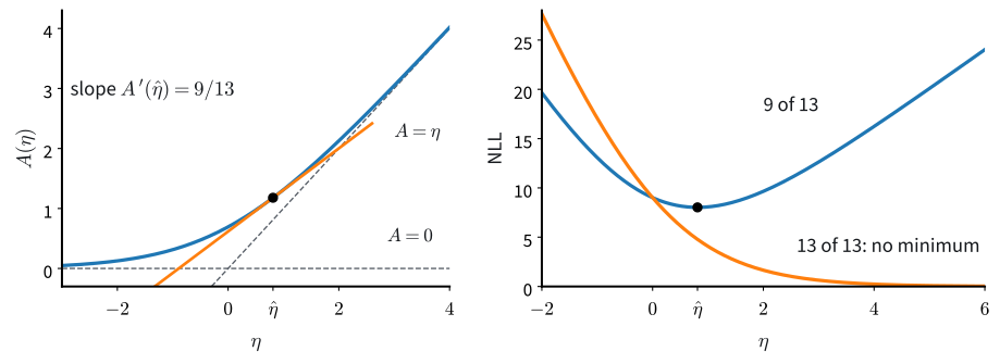
The equation \(\nabla A(\hat{\boldsymbol\eta})=\bar T\) has a solution only if \(\bar T\) is a mean that some member of the family attains. For the coin the attainable means are \(\operatorname{sigmoid}(\eta)\) for real \(\eta\), the open interval \((0,1)\). If all 13 flips are heads, \(\bar T=1\) is not attainable. The negative log-likelihood is then \(13A(\eta)-13\eta=13\log(1+e^{-\eta})\), which decreases for every \(\eta\): it is \(9.01\) at \(\eta=0\), \(0.087\) at \(\eta=5\) and \(0.0006\) at \(\eta=10\). It approaches \(0\) without reaching it, so there is no minimizer; the fitted bias runs to \(1\) and \(\hat\eta\) to infinity.
Logistic regression fails in the same way when a hyperplane separates the two classes of the training data: the loss keeps falling as the weights grow, and the weights grow without bound. A prior on the parameters, which we meet at the end of this section, or weight decay restores a finite solution; Exercise 9 computes it.
When a solution exists, it is unique if the negative log-likelihood is strictly convex, which requires \(\textrm{Cov}(T)\) to be positive definite. This holds when no linear combination of the statistics is constant, which is called a minimal representation. The categorical distribution with all \(K\) logits as natural parameters is not minimal: the one-hot statistics sum to one, and adding the same constant to every logit leaves every probability unchanged. Its negative log-likelihood is flat along the direction \(\mathbf 1\), and its minimizers form a line. Deep-learning implementations keep all \(K\) logits and use the same invariance to subtract the largest logit before exponentiating, which prevents overflow (Section 3.5).
27.3.3.3 Generalized Linear Models
Regression and classification models predict a distribution of a label \(y\) for each input \(\mathbf x\). A generalized linear model takes that distribution from an exponential family and makes its natural parameter a linear function of the input, \(\boldsymbol\eta = \mathbf W^\top\mathbf x\) (a bias is a constant feature). Write \(\boldsymbol\mu(\mathbf x) = \nabla A(\boldsymbol\eta) = \mathbb{E}[T(y)\mid\mathbf x]\) for the model’s mean of the sufficient statistic. The negative log-likelihood of one example is \(A(\boldsymbol\eta) - \boldsymbol\eta^\top T(y) - \log h(y)\), so by the moment property its gradient with respect to \(\boldsymbol\eta\) is \(\boldsymbol\mu(\mathbf x) - T(y)\), and the chain rule through \(\boldsymbol\eta = \mathbf W^\top\mathbf x\) gives
\[ \nabla_{\mathbf W}\bigl(-\log p(y\mid\mathbf x)\bigr) = \mathbf x\,\bigl(\boldsymbol\mu(\mathbf x) - T(y)\bigr)^\top . \tag{27.3.5}\]
The gradient is the input times the error of the predicted mean: prediction minus observation, whatever the family. The loss is convex in \(\mathbf W\), because it is the convex function \(A\) composed with a linear function of \(\mathbf W\), plus a term linear in \(\mathbf W\). Four families give four familiar models:
| label \(y\) | family | \(T(y)\) | mean \(\boldsymbol\mu(\mathbf x)\) | model |
|---|---|---|---|---|
| real number | Gaussian, variance 1 | \(y\) | \(\eta\) | linear regression |
| yes or no | Bernoulli | \(y \in \{0, 1\}\) | \(\operatorname{sigmoid}(\eta)\) | logistic regression |
| one of \(K\) classes | categorical | one-hot \(\mathbf y\) | \(\mathrm{softmax}(\boldsymbol\eta)\) | softmax regression |
| count | Poisson | \(y\) | \(e^{\eta}\) | Poisson regression |
A count model shows the rule at work. Suppose a Poisson model predicts the mean \(e^\eta=3\) for some input and the observed count is \(y=5\). The gradient of the loss with respect to \(\eta\) is \(3-5=-2\), so a gradient step raises \(\eta\) and with it the predicted mean, and the gradient with respect to the weights is \(-2\mathbf x\).
With variance \(\sigma^2\) instead of 1, the Gaussian negative log-likelihood is \((\hat y - y)^2/(2\sigma^2)\) plus a constant, where \(\hat y = \mathbf w^\top\mathbf x\): the squared loss of Section 2.1 divided by \(\sigma^2\), with the gradient \(\mathbf x(\hat y - y)/\sigma^2\). Softmax regression in Section 3.1 has the gradient \(\mathbf x(\hat{\mathbf y} - \mathbf y)^\top\) for the same reason. A neural network keeps the last step, a linear map into the natural parameters followed by the family’s negative log-likelihood, and replaces the fixed input \(\mathbf x\) by learned features. The loss is then no longer convex in the weights, but its gradient with respect to the natural parameters is still prediction minus observation (Bishop 2006).
27.3.4 Origins of the Softmax
Every multiclass classifier of the main text turns its \(K\) logits \(\mathbf z\) into class probabilities with the softmax,
\[ \mathrm{softmax}(\mathbf z)_k = \frac{e^{z_k}}{\sum_{j=1}^K e^{z_j}}, \qquad k=1,\dots,K. \tag{27.3.6}\]
The categorical rows of both tables above lead to the same map. Each probability grows with its own logit, and the probabilities sum to one. Other maps share these properties: normalizing \(\log(1+e^{z_k})\) instead of \(e^{z_k}\) also gives positive numbers that sum to one and keep the order of the logits. Under the softmax, however, \(z_i-z_j=\log(p_i/p_j)\) is a log-ratio of probabilities. Three arguments from different fields lead to this choice: a model of noisy choices, the Boltzmann distribution of physics, and the exponential family.
27.3.4.1 Noisy Choices and Gumbel Noise
The first argument starts from how labels come about. Suppose that a decision maker, such as a shopper or whoever labels our data, gives each option \(k\) a score \(z_k\) but does not always pick the best one. A simple model of this behavior perturbs every score by independent noise \(\epsilon_k\) and picks the largest perturbed score,
\[ y = \operatorname*{argmax}_{k}\,(z_k+\epsilon_k). \]
The probability of class \(k\) is the chance that option \(k\) wins this noisy contest, so the noise distribution decides its form. Psychologists modeled judgments in this way, with Gaussian errors, long before machine learning. With two options and \(\epsilon_k\sim\mathcal N(0,s^2)\), option 1 wins when \(\epsilon_2-\epsilon_1<z_1-z_2\). The difference \(\epsilon_2-\epsilon_1\) is Gaussian with variance \(2s^2\), so
\[ P(y=1) = \Phi\Bigl(\frac{z_1-z_2}{\sqrt2\,s}\Bigr), \]
where \(\Phi\) is the standard Gaussian CDF. This is the probit model: the probability depends only on the score difference, measured in units of the noise.
With more than two options the probit model has no closed form. Let \(\phi\) be the standard Gaussian density. Option \(k\) wins when every other perturbed score falls below its own, and averaging this chance over the standardized noise \(u=\epsilon_k/s\) of option \(k\) gives
\[ P(y=k) = \int_{-\infty}^{\infty}\phi(u)\prod_{j\ne k}\Phi\Bigl(u+\frac{z_k-z_j}{s}\Bigr)\,du . \]
For \(K>2\) this integral and its gradient must be computed numerically, for every example at every training step.
Gumbel noise removes the integral. The standard Gumbel distribution has the CDF \(G(x)=\exp(-e^{-x})\). It is the limiting distribution of the suitably shifted and scaled maximum of many independent draws from unbounded distributions with exponentially decaying tails, such as the Gaussian or the exponential (Gumbel 1954), and McFadden (1974) used it as the noise in models of economic choices.
Proposition (Gumbel noise gives the softmax). If \(\epsilon_1,\dots,\epsilon_K\) are independent standard Gumbel variables, the noisy argmax follows the softmax probabilities,
\[ P\Bigl(\operatorname*{argmax}_j\,(z_j+\epsilon_j)=k\Bigr) = \frac{e^{z_k}}{\sum_{j=1}^K e^{z_j}} . \]
Proof. Write \(S=\sum_j e^{z_j}\). The perturbed score \(z_j+\epsilon_j\) has the CDF \(G(t-z_j)=\exp(-e^{z_j}e^{-t})\). If option \(k\) scores \(t=z_k+\epsilon_k\), it wins with probability \(\prod_{j\ne k}\exp(-e^{z_j}e^{-t})=\exp\bigl(-(S-e^{z_k})e^{-t}\bigr)\), by independence. We multiply by the density \(e^{z_k}e^{-t}\exp(-e^{z_k}e^{-t})\) of \(t\), integrate, and substitute \(v=e^{-t}\):
\[ P(y=k) = \int_{-\infty}^{\infty} e^{z_k}e^{-t}\exp\bigl(-Se^{-t}\bigr)\,dt = e^{z_k}\int_0^{\infty} e^{-Sv}\,dv = \frac{e^{z_k}}{S} . \quad\blacksquare \]
The proof works because a product of Gumbel CDFs is again a Gumbel CDF. Over all \(K\) options, \(P\bigl(\max_j(z_j+\epsilon_j)\le t\bigr)=\exp(-Se^{-t})=G(t-\log S)\), so the winning score is a standard Gumbel variable shifted by the log-sum-exp \(\log\sum_j e^{z_j}\). The log-sum-exp is thus a smoothed maximum of the logits, and its gradient, the softmax, gives the chance that each option attains the maximum. Exercise 1 proves the proposition a second way, through races between exponential waiting times.
Read from right to left, the proposition is a sampler: to draw a class with the softmax probabilities, add independent Gumbel noise to the logits and take the argmax. This is the Gumbel-max trick.
Because \(\operatorname{argmax}_k(z_k+T\epsilon_k)=\operatorname{argmax}_k(z_k/T+\epsilon_k)\) for \(T>0\), Gumbel noise of scale \(T\) samples from \(\mathrm{softmax}(\mathbf z/T)\): the amount of noise in the choice acts as a temperature. To check both statements by simulation, we add Gumbel noise of scale \(T=1\) and \(T=2\) to four logits \(10^5\) times and count how often each option wins.
z = np.array([2.0, 1.0, 0.1, -1.0])                      # four logits
softmax = lambda v: np.exp(v) / np.exp(v).sum()
rng = np.random.default_rng()
n = 100_000
for T in (1.0, 2.0):                                      # noise scale = temperature
    winners = np.argmax(z + T * rng.gumbel(size=(n, 4)), axis=1)
    freq = np.bincount(winners, minlength=4) / n
    print(f'T = {T:.0f}: argmax frequencies {freq.round(3)}')
    print(f'      softmax(z / T)        {softmax(z / T).round(3)}'
f' max diff {np.abs(freq - softmax(z / T)).max():.3f}')T = 1: argmax frequencies [0.639 0.236 0.094 0.031]
softmax(z / T) [0.638 0.235 0.095 0.032] max diff 0.001
T = 2: argmax frequencies [0.453 0.274 0.172 0.101]
softmax(z / T) [0.451 0.274 0.174 0.101] max diff 0.002T = 1: argmax frequencies [0.639 0.236 0.094 0.031]
softmax(z / T) [0.638 0.235 0.095 0.032] max diff 0.001
T = 2: argmax frequencies [0.453 0.276 0.173 0.099]
softmax(z / T) [0.451 0.274 0.174 0.101] max diff 0.002T = 1: argmax frequencies [0.637 0.235 0.096 0.033]
softmax(z / T) [0.638 0.235 0.095 0.032] max diff 0.001
T = 2: argmax frequencies [0.453 0.273 0.172 0.101]
softmax(z / T) [0.451 0.274 0.174 0.101] max diff 0.002T = 1: argmax frequencies [0.638 0.234 0.097 0.031]
softmax(z / T) [0.638 0.235 0.095 0.032] max diff 0.001
T = 2: argmax frequencies [0.448 0.275 0.174 0.102]
softmax(z / T) [0.451 0.274 0.174 0.101] max diff 0.003The frequencies differ from \(\mathrm{softmax}(\mathbf z/T)\) by a few thousandths, the size of the Monte Carlo error for \(10^5\) draws. Doubling the noise flattens the frequencies in the same way as halving the logits.
With two options, the difference of two independent standard Gumbel variables has the logistic distribution, whose CDF is \(\operatorname{sigmoid}(x)=1/(1+e^{-x})\), so this logit model gives \(P(y=1)=\operatorname{sigmoid}(z_1-z_2)\). The sigmoid is close to a rescaled Gaussian CDF, \(|\operatorname{sigmoid}(1.7x)-\Phi(x)|<0.01\) for all \(x\), so fitted probit and logit models give nearly the same probabilities and differ mainly in the scale of their scores. They differ in the tails, which decay like \(e^{-x}\) for the logistic and like \(e^{-x^2/2}\) for the Gaussian. The negative log-likelihood of a confidently misclassified example therefore grows linearly in its score difference under the logit model and quadratically under the probit model, so mislabeled examples pull a probit fit harder (Exercise 4).
27.3.4.2 Temperature and the Boltzmann Distribution
The second argument comes from physics, where the same exponential appears for a different reason. A physical system in thermal equilibrium at temperature \(T\), such as a molecule in a gas, occupies a state \(k\) of energy \(E_k\) with probability
\[ p_k = \frac{\exp\bigl(-E_k/(k_{\mathrm B}T)\bigr)}{\sum_j \exp\bigl(-E_j/(k_{\mathrm B}T)\bigr)}, \]
where \(k_{\mathrm B}\) is Boltzmann’s constant. Low-energy states are the most probable, and the temperature sets how strongly they are preferred. Boltzmann found this law for the molecules of a gas, and Gibbs (1902) made it the basis of statistical mechanics. If we measure temperature in units of energy, so that \(k_{\mathrm B}=1\), and set \(E_k=-z_k\), the law becomes \(\mathrm{softmax}(\mathbf z/T)\). A logit is a negative energy, and the most probable class is the state of lowest energy. As \(T\to0\) the distribution concentrates on the largest logit; as \(T\to\infty\) it becomes uniform.
The maximum-entropy proposition explains this exponential without physics. Take the \(K\) classes as the outcomes, with \(h\equiv1\), and the logit \(z_k\) of class \(k\) as the statistic. Among all distributions on the classes with a given average logit \(\sum_k p_kz_k\), strictly between the smallest and the largest logit, the one of largest entropy is then \(p_k\propto e^{\eta z_k}\). For averages above the mean of the logits, \(\eta>0\), and this is \(\mathrm{softmax}(\mathbf z/T)\) with \(T=1/\eta\). As \(T\) falls from \(\infty\) to \(0\), the average logit rises from the mean of the logits to their maximum. For the logits \(\mathbf z=(2,1,0.1,-1)\) of the simulation, the plain softmax (\(T=1\)) has the average logit \(1.49\), between the mean \(0.525\) and the maximum \(2\).
27.3.4.3 The Categorical as an Exponential Family
The third argument is the one this section has already made. With the class written as a one-hot vector \(\mathbf y\), the categorical distribution is \(P(\mathbf y)=\exp\bigl(\mathbf z^\top\mathbf y-A(\mathbf z)\bigr)\) with \(A(\mathbf z)=\log\sum_ke^{z_k}\), an exponential family with the logits as natural parameters. By the moment property its mean is \(\nabla A(\mathbf z)=\mathrm{softmax}(\mathbf z)=\mathbb{E}[\mathbf y]\). Its negative log-likelihood is convex in the logits, and by Equation 27.3.5 its gradient is \(\mathrm{softmax}(\mathbf z)-\mathbf y\).
The three arguments agree on the function and explain different things about it. Noisy choices give the labels a generative model and an exact sampler. The Boltzmann distribution gives the temperature and the maximum-entropy reading. The exponential family gives the convex loss and its gradient.
27.3.5 Conjugate Priors
Maximum likelihood turns 9 heads in 13 flips into one number, \(9/13\). One number says nothing about how far to trust it: 9 heads in 13 flips and 900 in 1300 give the same estimate. A distribution over the bias would carry this information, and it should absorb the next flip by a small update rather than a new calculation.
From here on the bias is an unknown quantity with a distribution of its own, and as in the rest of the chapter we write it \(\theta\). A distribution over \(\theta\) before the data is a prior. Bayes’ rule multiplies it by the likelihood and normalizes the product, \(p(\theta\mid x)\propto p(\theta)\,P(x\mid\theta)\), which gives the posterior. A prior is conjugate to a likelihood if the posterior has the same functional form as the prior, so that observing data changes only its parameters.
27.3.5.1 The Beta Prior on a Coin
A prior on a coin’s bias is a density on \([0,1]\). As a function of \(\theta\), the likelihood of \(x\) heads in \(n\) flips is \(\theta^x(1-\theta)^{n-x}\), so a prior with the same shape combines with it by adding exponents. Its normalizer uses the Gamma function \(\Gamma(z)=\int_0^\infty t^{z-1}e^{-t}\,dt\) for \(z>0\), which extends the factorial: integration by parts gives \(\Gamma(z+1)=z\,\Gamma(z)\), and with \(\Gamma(1)=1\) this yields \(\Gamma(n+1)=n!\). The Beta distribution with parameters \(a,b>0\) has the density
\[ \mathrm{Beta}(\theta\mid a,b) = \frac{\theta^{a-1}(1-\theta)^{b-1}}{B(a,b)}, \qquad 0\le\theta\le1, \tag{27.3.7}\]
where the normalizer \(B(a,b)=\int_0^1\theta^{a-1}(1-\theta)^{b-1}d\theta\) equals \(\Gamma(a)\Gamma(b)/\Gamma(a+b)\). The mean follows from the normalizer, because multiplying the density by \(\theta\) raises \(a\) by one:
\[ \mathbb{E}[\theta] = \frac{1}{B(a,b)}\int_0^1 \theta^{a}(1-\theta)^{b-1}\,d\theta = \frac{B(a+1,b)}{B(a,b)} = \frac{a}{a+b}, \]
using \(\Gamma(a+1)=a\,\Gamma(a)\) and \(\Gamma(a+b+1)=(a+b)\Gamma(a+b)\) to simplify the ratio. The same step applied twice gives the variance. With \(m=a/(a+b)\) the prior mean,
\[ \textrm{Var}(\theta) = \frac{ab}{(a+b)^2(a+b+1)} = \frac{m(1-m)}{a+b+1}. \]
The variance is that of a single flip with bias \(m\), divided by \(a+b+1\): the larger \(a+b\), the more concentrated the prior. The case \(a=b=1\) is the uniform density on \([0,1]\).
Now we observe \(x\) heads in \(n\) flips. Multiplying the prior by the likelihood adds the exponents,
\[ \underbrace{\theta^{a-1}(1-\theta)^{b-1}}_{\text{prior}}\cdot \underbrace{\theta^{x}(1-\theta)^{n-x}}_{\text{likelihood}} = \theta^{(a+x)-1}(1-\theta)^{(b+n-x)-1}, \]
which, up to normalization, is again a Beta density, with parameters shifted by the data:
\[ \theta \mid x \;\sim\; \mathrm{Beta}\bigl(a+x,\ b+n-x\bigr). \tag{27.3.8}\]
This update has a pseudo-count interpretation. The parameters \(a\) and \(b\) act as prior counts of heads and tails, and observing \(x\) heads and \(n-x\) tails adds these to the counts. The posterior mean
\[ \mathbb{E}[\theta\mid x] = \frac{a+x}{a+b+n} \]
is the frequency of heads after including the pseudo-counts. It lies between the prior mean \(a/(a+b)\) and the maximum-likelihood estimate \(x/n\), and approaches the latter as \(n\) grows.
For the chapter’s coin with the uniform prior \(\mathrm{Beta}(1,1)\), 9 heads in 13 flips give the posterior \(\mathrm{Beta}(10,5)\). Its mean is \(10/15=2/3\), which is Laplace’s rule of succession \((x+1)/(n+2)\) (Laplace 1814): add one imagined head and one imagined tail. Its mode \((a+x-1)/(a+b+n-2)=9/13\) is the maximum-likelihood estimate, and its standard deviation is \(\sqrt{(2/3)(1/3)/16}\approx0.118\).
After 90 heads in 130 flips the posterior is \(\mathrm{Beta}(91,41)\), with mean \(0.689\) and standard deviation \(0.040\). Ten times as many flips shrink the standard deviation by a factor of \(2.9\). The posterior mean barely moved, while \(a+b+1\) grew from \(16\) to \(133\), and \(\sqrt{133/16}\approx2.9\). This is the \(1/\sqrt n\) law for posterior widths.
The posterior also answers a practical question: what is the probability that the next flip is heads? Given \(\theta\) it is \(\theta\), and averaging over the posterior gives \(P(\text{heads}\mid x)=\int_0^1\theta\,p(\theta\mid x)\,d\theta=\mathbb{E}[\theta\mid x]\). For the coin this is \(2/3\), so Laplace’s rule is the predicted probability of the next head.
Is the normalized product of prior and likelihood the \(\mathrm{Beta}(10,5)\) density, and does it have mean \(2/3\) and standard deviation \(0.118\)? We multiply the flat prior by the likelihood on a fine grid of \(\theta\), normalize the product numerically, and compare it with the closed form.
a, b, x, n = 1, 1, 9, 13                                  # Beta(1,1) prior; 9 heads in 13
theta = np.linspace(0, 1, 100_001)[1:-1]                  # interior grid points
dtheta = theta[1] - theta[0]
post = theta**(a - 1) * (1 - theta)**(b - 1) * theta**x * (1 - theta)**(n - x)
post /= post.sum() * dtheta                               # normalize numerically
log_B = math.lgamma(a + x) + math.lgamma(b + n - x) - math.lgamma(a + b + n)
beta = np.exp((a + x - 1) * np.log(theta) + (b + n - x - 1) * np.log1p(-theta) - log_B)
mean = (theta * post).sum() * dtheta
sd = math.sqrt(((theta - mean)**2 * post).sum() * dtheta)
print(f'max |prior * likelihood - Beta({a + x},{b + n - x})| = {np.abs(post - beta).max():.1e}')
print(f'posterior mean = {mean:.3f}, sd = {sd:.3f}')
max |prior * likelihood - Beta(10,5)| = 2.1e-14
posterior mean = 0.667, sd = 0.118The normalized product and the \(\mathrm{Beta}(10,5)\) density agree to rounding error, far below \(10^{-8}\), with mean \(0.667\) and standard deviation \(0.118\). Figure 27.3.3 follows the update further.

27.3.5.2 Conjugacy for Every Exponential Family
The Beta update looks like a lucky match of exponents. It is an instance of a general fact: every exponential family has a conjugate prior, and the update always adds the sufficient statistics.
Proposition (conjugate prior). Consider a likelihood Equation 27.3.1 and the prior on the natural parameters
\[ p(\boldsymbol\eta) \propto \exp\bigl(\boldsymbol\nu^\top\boldsymbol\eta - \kappa\,A(\boldsymbol\eta)\bigr), \tag{27.3.9}\]
with \(\boldsymbol\nu\in\mathbb R^d\) and \(\kappa\in\mathbb R\) chosen such that this density is normalizable. After \(n\) independent observations \(\mathbf x_1,\dots,\mathbf x_n\), the posterior has the same form, with \(\boldsymbol\nu\) replaced by \(\boldsymbol\nu+\sum_iT(\mathbf x_i)\) and \(\kappa\) by \(\kappa+n\).
Proof. The likelihood contributes \(\exp(\boldsymbol\eta^\top\sum_iT(\mathbf x_i)-nA(\boldsymbol\eta))\) times a factor that does not depend on \(\boldsymbol\eta\), so
\[ e^{\boldsymbol\nu^\top\boldsymbol\eta-\kappa A(\boldsymbol\eta)}\cdot e^{\boldsymbol\eta^\top\sum_iT(\mathbf x_i)-nA(\boldsymbol\eta)} = e^{(\boldsymbol\nu+\sum_iT(\mathbf x_i))^\top\boldsymbol\eta-(\kappa+n)A(\boldsymbol\eta)} . \]
Normalizing the product gives the posterior, so the posterior has the prior’s form with the updated \(\boldsymbol\nu\) and \(\kappa\). \(\blacksquare\)
The normalizer of the posterior is the probability of the data. It is finite for discrete data, where the likelihood is at most one, and for almost every data set in general.
The prior’s own parameters \(\boldsymbol\nu\) and \(\kappa\), called hyperparameters, act as pseudo-data: \(\boldsymbol\nu\) is a prior total of the sufficient statistic and \(\kappa\) a prior sample size (Bishop 2006). For the coin the prior lives on the logit \(\eta=\log\frac{\theta}{1-\theta}\), and a change of variables from \(\eta\) to \(\theta\) turns it into \(\mathrm{Beta}(\nu,\kappa-\nu)\) on \(\theta\); the update \(\nu\to\nu+x\), \(\kappa\to\kappa+n\) is the Beta update \(a\to a+x\), \(b\to b+n-x\). Exercise 7 carries out the change of variables, including its Jacobian.
27.3.5.3 Gamma–Poisson and Dirichlet–Multinomial
Two more pairs follow the same recipe and appear later in the book: one for rates of events, one for the probabilities of words. The Gamma distribution with shape \(a>0\) and rate \(b>0\) is the density \(\mathrm{Gamma}(\lambda\mid a,b)=\frac{b^a}{\Gamma(a)}\lambda^{a-1}e^{-b\lambda}\) on \(\lambda>0\), with mean \(a/b\) and variance \(a/b^2\). As a function of the rate, \(n\) Poisson counts \(x_1,\dots,x_n\) have the likelihood \(\prod_i\lambda^{x_i}e^{-\lambda}/x_i!\propto\lambda^{\sum_ix_i}e^{-n\lambda}\), and multiplying by the prior collects the powers into the posterior \(\mathrm{Gamma}\bigl(a+\sum_ix_i,\ b+n\bigr)\). The shape counts events and the rate counts observation periods, so the prior acts as \(a\) imagined events in \(b\) imagined periods. Averaging the Poisson over a Gamma-distributed rate gives the negative binomial, a count distribution whose variance exceeds its mean.
The Dirichlet distribution is a density on probability vectors \(\mathbf p\) with \(K\) entries, \(p_k\ge0\) and \(\sum_kp_k=1\). With parameters \(a_k>0\) it is
\[ \mathrm{Dir}(\mathbf p\mid\mathbf a)=\frac{\Gamma(\sum_ka_k)}{\prod_k\Gamma(a_k)}\prod_{k=1}^K p_k^{a_k-1}, \]
with mean \(\mathbb{E}[p_k]=a_k/\sum_ja_j\); for \(K=2\) it is the Beta distribution. Counts \(x_1,\dots,x_K\) of the \(K\) categories have the likelihood \(\prod_kp_k^{x_k}\), so the posterior is \(\mathrm{Dir}(\mathbf a+\mathbf x)\): one pseudo-count per category.
Suppose a three-word vocabulary shows the counts \((3,0,1)\). The maximum-likelihood estimate \((0.75,0,0.25)\) gives the unseen second word probability zero, and any text containing it becomes impossible. Under the prior \(\mathrm{Dir}(1,1,1)\) the posterior is \(\mathrm{Dir}(4,1,2)\), with mean \((4/7,1/7,2/7)\approx(0.571,0.143,0.286)\). Adding one to every count before normalizing is called add-one smoothing, and it is the posterior mean under this prior.
We can now write the distribution of a binary, categorical, count, waiting-time or real-valued label in one form and read its mean and variance off the derivatives of \(A\). We can fit it by maximum likelihood as a convex problem that matches the average statistic, as \(\operatorname{sigmoid}(\hat\eta)=9/13\) does for the coin. We can also update a conjugate prior by adding counts, from \(\mathrm{Beta}(1,1)\) to \(\mathrm{Beta}(10,5)\). Two gaps remain. When the moment equation has no finite solution, a prior restores an estimate, and when the posterior has no closed form, it must be computed numerically; later sections of this chapter develop both. And an estimate from 13 flips is a number without an error bar: how far can \(9/13\) be from the true bias, and do two coins with 9 and 11 heads in 13 flips differ? Section 27.4 takes up these questions.
27.3.6 Summary
Nearly every distribution of the catalogue has the form \(h(\mathbf x)\exp(\boldsymbol\eta^\top T(\mathbf x)-A(\boldsymbol\eta))\), in which the data and the parameters meet only in the inner product \(\boldsymbol\eta^\top T(\mathbf x)\); the uniform and the Student-\(t\) are the main exceptions. Maximum entropy produces this form when only the averages of the statistics are fixed. The log-partition function generates moments: \(\nabla A\) is the mean of \(T\) and \(\nabla^2A\) its covariance, so \(A\) is convex. Maximum likelihood is therefore a convex problem that matches the mean of \(T\) to its sample average whenever that average is attainable. A generalized linear model trains with the gradient input times prediction minus observation, which is why linear, logistic, softmax and Poisson regression share one rule. The softmax arises as the choice under Gumbel noise, as the Boltzmann distribution, and as the mean of the categorical family. Every exponential family has a conjugate prior whose update adds the sufficient statistics to pseudo-counts, as in the step from \(\mathrm{Beta}(1,1)\) to \(\mathrm{Beta}(10,5)\) for the coin.
27.3.7 Exercises
- Exponential races. Let \(X_1,\dots,X_m\) be independent with \(X_i\sim\mathrm{Exp}(\lambda_i)\), for example the waiting times for the next event in \(m\) independent event streams.
- Show that \(\min_i X_i\sim\mathrm{Exp}\bigl(\sum_i\lambda_i\bigr)\).
- Show that the \(j\)-th stream fires first with probability \(P\bigl(X_j=\min_i X_i\bigr)=\lambda_j/\sum_i\lambda_i\).
- Let \(V_1,\dots,V_K\) be independent \(\mathrm{Exp}(1)\) variables and let \(\mathbf z\in\mathbb R^K\) be a vector of logits. Use (b) to show that \(\operatorname{argmax}_k\,(z_k-\log V_k)\) is distributed according to the softmax probabilities Equation 27.3.6. Because \(-\log V_k\) has the standard Gumbel distribution, this is a second proof that Gumbel noise gives the softmax.
- Maximum entropy on the integers. Consider distributions \((p_0,p_1,p_2,\dots)\) on \(\{0,1,2,\dots\}\) with a fixed mean \(m>0\).
- Maximize the Shannon entropy \(H[p]=-\sum_k p_k\log p_k\) subject to \(\sum_k p_k=1\) and \(\sum_k k\,p_k=m\), using Lagrange multipliers (Section 26.5.1). Show that the stationary point is a geometric distribution \(p_k=(1-r)\,r^k\), and express \(r\) through \(m\).
- Repeat the derivation for the entropy relative to \(h(k)=1/k!\), \(H_h[p]=-\sum_k p_k\log\bigl(p_k/h(k)\bigr)\), and show that the stationary point is \(\mathrm{Poisson}(m)\).
- At \(m=4\), compute the Shannon entropy of both distributions numerically. Which one is larger, and why must it be? Compare \(P(X\ge15)\) under the two distributions. Which assumption about large counts does the choice of base measure encode?
- A stationary point of a Lagrangian need not be a maximum. Use the maximum-entropy proposition to prove that the two distributions of
- and (b) are the global maximizers, by exhibiting each as a member of an exponential family whose mean equals \(m\).
- Moments from the log-partition. The moment property Equation 27.3.3 and its second-order form \(\nabla^2A=\textrm{Cov}(T)\) turn moment calculations into differentiation.
- For the Poisson, \(A(\eta)=e^\eta\). Derive the mean and the variance from \(A\). Which property of the function \(A\) makes them equal?
- For the Gaussian, the natural parameters are \(\eta_1=\mu/\sigma^2\) and \(\eta_2=-1/(2\sigma^2)\). Show that \(A=-\eta_1^2/(4\eta_2)-\frac12\log(-2\eta_2)\), and differentiate it to recover \(\mathbb{E}[x]\), \(\mathbb{E}[x^2]\), \(\textrm{Var}(x)\) and \(\textrm{Cov}(x,x^2)\).
- The Laplace distribution with a fixed location \(\mu\) and scale \(b\) has the sufficient statistic \(T(x)=|x-\mu|\). Write it in the form Equation 27.3.1, and use \(A\) to compute \(\mathbb{E}\,|x-\mu|\) and \(\textrm{Var}|x-\mu|\). Check the result against the Laplace variance \(2b^2\).
- For \(n\) Gaussian observations, write the two moment-matching equations \(\nabla A(\hat{\boldsymbol\eta})=\bar T\) and solve them for \(\hat\mu\) and \(\hat\sigma^2\). What happens for \(n=1\)? Relate your answer to the condition that \(\bar T\) be an attainable mean.
- [code] Probit and logit. For two classes with the score difference \(m=z_1-z_2\), the logit model gives \(P(y=1)=\operatorname{sigmoid}(m)\) and the probit model with noise scale \(s\) gives \(P(y=1)=\Phi\bigl(m/(\sqrt2\,s)\bigr)\).
- Show that the difference of two independent standard Gumbel variables has the CDF \(\operatorname{sigmoid}(x)\). The standard Gumbel distribution has variance \(\pi^2/6\). Find the scale \(c\) for which the distribution with CDF \(\operatorname{sigmoid}(cx)\) has variance 1, like the standard Gaussian.
- Find numerically the scale \(c\) that minimizes \(\max_x|\operatorname{sigmoid}(cx)-\Phi(x)|\), and the value of this maximum. Why is this scale smaller than the one of (a)?
- An example of class 2 lies on the wrong side of the decision boundary, with \(m>0\). Show that its negative log-likelihood \(-\log\operatorname{sigmoid}(-m)\) under the logit model lies between \(m\) and \(m+e^{-m}\), and that its derivative with respect to \(m\) is less than 1. Use the bounds \(\frac{x}{1+x^2}\,\phi(x)\le1-\Phi(x)\le\frac{\phi(x)}{x}\) for \(x>0\) to show that its negative log-likelihood \(-\log\Phi\bigl(-m/(\sqrt2\,s)\bigr)\) under the probit model grows like \(m^2/(4s^2)\), and that its derivative grows linearly in \(m\).
- Draw 100 inputs \(x\sim\mathcal N(1,1)\) of class 1 and 100 inputs \(x\sim\mathcal N(-1,1)\) of class 2, and let \(m=wx+b\). Fit \((w,b)\) by maximum likelihood under both models. Then add three examples at \(x=6\) labeled as class 2, and fit again. For each model, compute the ratio of the slope \(w\) with these mislabeled examples to the slope without them, and explain the difference between the models with (c). Compute \(\log\Phi\) with a numerically stable routine such as
scipy.special.log_ndtr.
- Minimal categorical family. ● Code a categorical outcome as a one-hot vector \(\mathbf x\in\{0,1\}^K\) with class probabilities \(\mathbf p=\mathrm{softmax}(\mathbf z)\), written as an exponential family with \(T(\mathbf x)=\mathbf x\), natural parameters \(\mathbf z\) and \(A(\mathbf z)=\log\sum_ke^{z_k}\).
- Compute \(\nabla^2 A(\mathbf z)\) and show that it equals the covariance \(\operatorname{diag}(\mathbf p)-\mathbf p\mathbf p^\top\) of the one-hot vector \(\mathbf x\). Every one-hot vector satisfies \(\mathbf x\mathbf x^\top=\operatorname{diag}(\mathbf x)\). Show that \(\nabla^2A(\mathbf z)\,\mathbf 1=\mathbf 0\), and that the gradient of the negative log-likelihood of a dataset is orthogonal to \(\mathbf 1\) at every \(\mathbf z\). Gradient descent with a small step size runs on the logits from a starting point \(\mathbf z_0\), and every class occurs in the data. Which function of \(\mathbf z\) does gradient descent never change? Which of the minimizers does it therefore approach?
- Fix \(z_K=0\). This gives a minimal representation with \(\boldsymbol\eta=(z_1,\dots,z_{K-1})\) and \(T(\mathbf x)=(x_1,\dots,x_{K-1})\). Show that \(\nabla^2A(\boldsymbol\eta)\) is positive definite whenever every \(p_k>0\). Given class counts \(n_1,\dots,n_K\), solve the moment-matching condition \(\nabla A(\hat{\boldsymbol\eta})=\bar T\) for the maximum-likelihood \(\hat{\boldsymbol\eta}\). What happens when some class has \(n_k=0\)?
- [code] Poisson regression. ● A generalized linear model for counts makes the natural parameter of a Poisson an affine function of the features: \(y_i\mid\mathbf x_i\sim\mathrm{Poisson}(e^{\eta_i})\) with \(\eta_i=\mathbf w^\top\mathbf x_i+b\).
- Use the negative log-likelihood Equation 27.3.4 to write the loss as a function of \((\mathbf w,b)\), and compute its gradient and Hessian. Show that the loss is convex. Which equations does a zero gradient impose on the fitted means \(\hat m_i=e^{\hat\eta_i}\)?
- Generate \(n=1000\) examples with \(\mathbf x_i\sim\mathcal N(\mathbf 0,\mathbf I_2)\), \(\mathbf w=(-0.3,1.0)\) and \(b=0.5\). Starting from zero, fit \(\mathbf u=(\mathbf w,b)\) with Newton’s method, which repeats the step \(\mathbf u\leftarrow\mathbf u-\bigl(\nabla^2L(\mathbf u)\bigr)^{-1}\nabla L(\mathbf u)\) for the loss \(L\), and check the equations of (a) at the solution.
- Multiply each rate by an independent \(g_i\sim\mathrm{Gamma}(1,1)\), which has mean \(1\), so that the counts become overdispersed while their conditional means stay \(e^{\eta_i}\). Fit the Poisson model to \(200\) such datasets and to \(200\) datasets without the multiplier. Compare the mean and the standard deviation of the estimates across datasets. Explain the behavior of the mean with the equations of (a).
- Conjugate priors from natural parameters. ● For a scalar natural parameter \(\eta\), the conjugate prior Equation 27.3.9 reads \(p(\eta)\propto\exp\bigl(\nu\,\eta-\kappa\,A(\eta)\bigr)\), and \(n\) observations update it by \(\nu\to\nu+\sum_i T(x_i)\) and \(\kappa\to\kappa+n\).
- For the Poisson, \(\eta=\log\lambda\) and \(A(\eta)=e^\eta\). Change variables from \(\eta\) to \(\lambda\), including the Jacobian, and show that the prior on \(\lambda\) is a Gamma distribution. Identify its shape and rate, and check that the update reproduces the Gamma posterior of Section 27.3.5.3.
- For the Bernoulli, \(\eta=\log\frac{\theta}{1-\theta}\) and \(A(\eta)=\log(1+e^\eta)\). Show that the prior on \(\theta\) is \(\mathrm{Beta}(\nu,\kappa-\nu)\), and find the values of \((\nu,\kappa)\) for which it is normalizable.
- Take the flat prior on the logit, \(\nu=\kappa=0\). Which density on \(\theta\) does it induce, and is that density normalizable? After \(x\) heads in \(n\) flips, when is the posterior normalizable, and what is its mean? Compare it with the mean of the posterior Equation 27.3.8 under the uniform prior \(\mathrm{Beta}(1,1)\) on \(\theta\). What does the comparison say about the phrase “a flat prior”?
- [code] Moment matching outside the family. Let \(x_1,\dots,x_n\) be independent draws from \(U(0,\theta)\).
- Write the likelihood and show that the maximum-likelihood estimate is \(\hat\theta_{\mathrm{ML}}=\max_ix_i\). Using the CDF \((t/\theta)^n\) of the maximum, show that \(\mathbb{E}[\hat\theta_{\mathrm{ML}}]=n\theta/(n+1)\) and \(\textrm{Var}(\hat\theta_{\mathrm{ML}})=n\theta^2/\bigl((n+1)^2(n+2)\bigr)\).
- Show that the moment estimate \(\hat\theta_{\mathrm{MM}}=2\bar x\) is unbiased with variance \(\theta^2/(3n)\).
- With \(\theta=1\), simulate \(20{,}000\) data sets for each of \(n=10,100,1000\) and report the root-mean-square error of both estimates. Which one falls like \(1/n\) and which like \(1/\sqrt n\)? Which property of the uniform distribution, absent in every exponential family, allows the faster rate?
- Show that \(n(\theta-\hat\theta_{\mathrm{ML}})\) converges in distribution to an exponential distribution with mean \(\theta\), and check the mean in your simulation at \(n=1000\).
- [code] A likelihood with no maximizer. This exercise follows the coin with 13 heads in 13 flips.
- Show that the negative log-likelihood in the logit is \(13\log(1+e^{-\eta})\), that it decreases for every \(\eta\) with infimum \(0\), and that it has no minimizer. What is \(\bar T\), and why is it not an attainable mean?
- Under the prior \(\mathrm{Beta}(2,2)\) the posterior is \(\mathrm{Beta}(15,2)\). Compute its mode and its mean, and explain why one imagined head and one imagined tail restore a solution strictly inside \((0,1)\).
- Logistic regression on the two examples \((x,y)=(1,1)\) and \((-1,0)\), with \(P(y=1\mid x)=\operatorname{sigmoid}(wx)\), has the negative log-likelihood \(2\log(1+e^{-w})\), which has no minimizer. Add the penalty \(\frac\lambda2w^2\) with \(\lambda=0.1\), show that the minimizer solves \(2\operatorname{sigmoid}(-w)=\lambda w\), solve this equation by bisection, and report \(w^\ast\) and the fitted probability \(\operatorname{sigmoid}(w^\ast)\). To which prior on \(w\) does the penalty correspond?
- Dirichlet smoothing and the next word. A three-word vocabulary shows the counts \(\mathbf c=(3,0,1)\), and the prior is \(\mathrm{Dir}(1,1,1)\).
- Write the posterior and its mean, and compare the mean with the maximum-likelihood estimate.
- Show that the probability that the next word is word \(k\), \(\int p_k\,\mathrm{Dir}(\mathbf p\mid\mathbf a+\mathbf c)\,d\mathbf p\), equals the posterior mean \((a_k+c_k)/\sum_j(a_j+c_j)\). Use \(\Gamma(z+1)=z\,\Gamma(z)\) on the normalizer.
- For the prior \(\mathrm{Dir}(s,\dots,s)\) on \(K\) words, show that the posterior mean tends to the maximum-likelihood estimate as \(s\to0\) and to the uniform distribution as \(s\to\infty\).
- A corpus has \(10^6\) words and a vocabulary of \(50{,}000\), of which \(20{,}000\) never occur. With add-one smoothing (\(s=1\)), by what factor does the estimate for a word seen \(5\) times change, and what total probability do the unseen words receive?