import numpy as np33.4 Spectra in Practice
The matrices of Section 33.3 were small enough to solve by hand, and we trusted what their eigenvalues told us: the surfer’s error shrank by the factor \(1/4\) at every click, as the second eigenvalue said it would. Both comforts end outside the textbook. The link matrix of the web has billions of rows, and nobody writes down its characteristic polynomial. And eigenvalues promise less than they seem to. A Jordan block whose eigenvalues are both \(0.99\) grew to norm 37 before it decayed (Section 33.3.1.5), and backpropagation through a recurrent network multiplies the gradient by fifty different matrices, where the surfer applied one matrix fifty times.
This section takes the two problems in turn. First, what can we learn about the eigenvalues of a matrix that is too large to factor? Surprisingly much: the entries alone confine the eigenvalues to a few discs, and repeated multiplication by the matrix, the one operation that stays cheap, finds the largest eigenvalue and its eigenvector. PageRank was computed this way. Second, what do eigenvalues leave unsaid about a finite number of steps, or about a product of different matrices? Here the answer is sobering. Eigenvalues describe the long run of the powers of one matrix. For anything else we need norms, and in the end the singular values of Section 33.5.
The topics are not of equal weight. Three recur in deep learning. Power iteration (Section 33.4.1.2) estimates the largest stretch of a layer for spectral normalization (Section 33.5.4.3). Transient growth and products of Jacobians (Section 33.4.2.3, Section 33.4.2.5) are the mathematics of the exploding and vanishing gradients of Section 8.6. The random matrices of Section 33.4.2.6 are the weight matrices of Section 4.4 at initialization. Gershgorin’s theorem and PageRank are classical, and deep learning uses them less often; a reader in a hurry may skim both. Pseudospectra (Section 33.4.2.4) are a diagnostic that few readers will compute, and can be skipped as well. The computations use NumPy.
import numpy as npimport numpy as npimport numpy as np33.4.1 Locating and Computing Eigenvalues
33.4.1.1 Gershgorin Discs
Can we say where the eigenvalues of a matrix lie without computing them? For a diagonal matrix they are the diagonal entries. If the off-diagonal entries are small, the eigenvalues should stay near the diagonal, and the following theorem says how near.
Theorem (Gershgorin (Gershgorin 1931)). Let \(\mathbf{A}=(a_{ij})\) be any \(n\times n\) matrix and let \(r_i=\sum_{j\neq i}|a_{ij}|\) be the sum of the absolute values of the off-diagonal entries in row \(i\). Let \(\mathcal{D}_i\) be the disc in the complex plane with centre \(a_{ii}\) and radius \(r_i\). Then every eigenvalue of \(\mathbf{A}\) lies in the union \(\bigcup_i\mathcal{D}_i\).
Proof. Let \(\mathbf{A}\mathbf{v}=\lambda\mathbf{v}\) with \(\mathbf{v}\neq\mathbf 0\), and pick the index \(i\) of an entry of largest magnitude, so that \(|v_i|\ge|v_j|\) for all \(j\) and \(v_i\neq0\). Row \(i\) of \(\mathbf{A}\mathbf{v}=\lambda\mathbf{v}\) reads
\[ \sum_j a_{ij}v_j = \lambda v_i \quad\Longrightarrow\quad (\lambda - a_{ii})\,v_i = \sum_{j\neq i} a_{ij} v_j . \]
Divide by \(v_i\) and take absolute values; since each \(|v_j/v_i|\le1\),
\[ |\lambda - a_{ii}| = \Bigl|\sum_{j\neq i} a_{ij}\,\tfrac{v_j}{v_i}\Bigr| \le \sum_{j\neq i} |a_{ij}| = r_i , \]
so \(\lambda\in\mathcal{D}_i\). \(\blacksquare\)
The proof places each eigenvalue in the disc of the row where its eigenvector is largest, which we do not know in advance; the theorem therefore guarantees only the union. Consider the non-symmetric matrix
\[ \mathbf A=\begin{pmatrix}4&1&0\\-1&4&0.5\\0.5&0&1\end{pmatrix}. \tag{33.4.1}\]
The discs have centres 4, 4, 1 and radii 1, 1.5, 0.5. The two discs centred at 4 overlap (one contains the other), and the disc centred at 1 is disjoint from them, since \(|4-1|=3>1.5+0.5\). The eigenvalues are \(3.99\pm0.96i\) and \(1.03\): the complex pair lies inside the two discs centred at 4, and the real eigenvalue inside the small disc. Figure 33.4.1 draws the discs and the eigenvalues.

The split, two eigenvalues in the overlapping pair and one in the small disc, is not a coincidence. If a union of \(m\) discs is connected and disjoint from the other discs, it contains exactly \(m\) eigenvalues, counted with multiplicity, because eigenvalues move continuously as the off-diagonal entries grow from zero and cannot jump the gap between separated groups of discs (Horn and Johnson 2012). The cell computes the centres, radii and eigenvalues quoted above.
A = np.array([[4.0, 1.0, 0.0],
              [-1.0, 4.0, 0.5],
              [0.5, 0.0, 1.0]])
centres = np.diag(A)
radii = np.abs(A).sum(axis=1) - np.abs(centres)
print('centres:', centres, '  radii:', radii)
for z in np.linalg.eigvals(A):
    print(f'eigenvalue {z:.3f}   distances to the centres: '
          f'{np.abs(z - centres).round(2)}')
centres: [4. 4. 1.] radii: [1. 1.5 0.5]
eigenvalue 3.987+0.961j distances to the centres: [0.96 0.96 3.14]
eigenvalue 3.987-0.961j distances to the centres: [0.96 0.96 3.14]
eigenvalue 1.025+0.000j distances to the centres: [2.97 2.97 0.03]The complex pair is at distance 0.96 from 4, close to the rim of the disc of radius 1: the theorem is nearly sharp here.
A corollary needs no computation at all. If \(\mathbf{A}\) is strictly diagonally dominant with positive diagonal, \(a_{ii}>r_i\) for every \(i\), then every disc lies in the open right half-plane, 0 is not an eigenvalue, and \(\mathbf A\) is invertible. If such a matrix is also symmetric, its eigenvalues are real and positive, so it is positive definite.
33.4.1.2 Power Iteration
A matrix with a billion rows cannot be factored, but it can be multiplied by a vector if it is sparse. What does \(\mathbf A^k\mathbf v_0\) tell us about its eigenvalues? The expansion Equation 33.3.4 answers this. Let \(\mathbf A\) be diagonalizable with eigenvectors \(\mathbf v_i\), ordered by modulus with a strictly dominant eigenvalue, \(|\lambda_1|>|\lambda_2|\ge\cdots\ge|\lambda_n|\). (For a real matrix, strict dominance forces \(\lambda_1\) to be real, since a complex eigenvalue would share its modulus with its conjugate.) Write \(\mathbf v_0=\sum_i c_i\mathbf v_i\) and factor out \(\lambda_1^k\):
\[ \mathbf{A}^k\mathbf{v}_0 = \sum_{i=1}^{n} c_i\lambda_i^k\mathbf{v}_i = \lambda_1^k\Bigl(c_1\mathbf{v}_1 + \sum_{i\ge2} c_i\Bigl(\tfrac{\lambda_i}{\lambda_1}\Bigr)^{k}\mathbf{v}_i\Bigr). \tag{33.4.2}\]
Every ratio \(|\lambda_i/\lambda_1|\) is below 1, so if \(c_1\neq0\) the bracket converges to \(c_1\mathbf v_1\). The direction of \(\mathbf A^k\mathbf v_0\) therefore approaches the eigenvector \(\mathbf v_1\), with an error that decays like \(|\lambda_2/\lambda_1|^k\), and the length grows by a factor approaching \(|\lambda_1|\) per step. Multiplying repeatedly and rescaling to length 1 after each step, so that the numbers stay in range, is power iteration (Golub and Van Loan 1996). For a symmetric matrix, the Rayleigh quotient of the iterate estimates \(\lambda_1\) and converges faster than the direction, at the squared rate \(|\lambda_2/\lambda_1|^{2k}\). The eigenvectors are orthogonal, so a misalignment of size \(\delta\) changes the Rayleigh quotient only by an amount of order \(\delta^2\) (Exercise 3).
Section 1.3 computed the iterates of \(\mathbf S\) from \(\mathbf e_1\): \((2,1)\), \((5,4)\), \((14,13)\), in general \(\bigl((3^k+1)/2,\,(3^k-1)/2\bigr)\). The expansion explains them. With the unit eigenvectors \(\mathbf v_1=(1,1)/\sqrt2\) and \(\mathbf v_2=(1,-1)/\sqrt2\), we have \(\mathbf e_1=(\mathbf v_1+\mathbf v_2)/\sqrt2\), so
\[ \mathbf S^k\mathbf e_1=\frac{3^k\mathbf v_1+\mathbf v_2}{\sqrt2}, \qquad \tan\angle(\mathbf S^k\mathbf e_1,\mathbf v_1)=3^{-k}, \qquad 3-R(\mathbf S^k\mathbf e_1)=\frac{2}{9^k+1}. \]
The direction error falls by the factor \(|\lambda_2/\lambda_1|=1/3\) per step: the sine of the angle to \(\mathbf v_1\) is 0.316, 0.110, 0.037 for \(k=1,2,3\). The error of the Rayleigh quotient falls by \(1/9\): it is 0.2, 0.024, 0.0027. Figure 33.4.2 plots both on a logarithmic scale.

Two conditions can fail. The start needs \(c_1\neq0\); a random start satisfies this with probability one. And the dominance must be strict. If the dominant eigenvalues are a complex pair of equal modulus, the dominant part of the iterate keeps rotating. The ratio of consecutive norms then oscillates forever, as it did for the running matrix of Section 33.3.1.6. Even then, the average rate \(\|\mathbf A^k\mathbf v_0\|^{1/k}\) converges to the largest modulus.
A matrix with positive entries is safe: it has a real, simple, strictly dominant eigenvalue, by the Perron–Frobenius theorem of Section 33.4.1.3. We run 200 steps of power iteration on a random \(5\times5\) matrix with entries uniform in \([0,1]\), from a random start, and compare the final norm ratio with the largest eigenvalue modulus.
A = np.random.rand(5, 5)                 # positive entries
v = np.random.randn(5)
for _ in range(200):
    Av = A @ v
    ratio = np.linalg.norm(Av) / np.linalg.norm(v)
    v = Av / np.linalg.norm(Av)
mods = np.sort(np.abs(np.linalg.eigvals(A)))[::-1]
print(f'norm ratio after 200 steps = {ratio:.10f}')
print(f'largest |eigenvalue|       = {mods[0]:.10f}')
print(f'|lambda_2| / |lambda_1| = {mods[1] / mods[0]:.3f}')norm ratio after 200 steps = 2.5254088042
largest |eigenvalue| = 2.5254088042
|lambda_2| / |lambda_1| = 0.299norm ratio after 200 steps = 1.9587653322
largest |eigenvalue| = 1.9587653322
|lambda_2| / |lambda_1| = 0.370norm ratio after 200 steps = 2.5650940439
largest |eigenvalue| = 2.5650940439
|lambda_2| / |lambda_1| = 0.127norm ratio after 200 steps = 2.2727569166
largest |eigenvalue| = 2.2727569166
|lambda_2| / |lambda_1| = 0.188The norm ratio agrees with the largest eigenvalue modulus in every printed digit, on every run. One draw does not show how typical this is, so we compute the gap ratio \(|\lambda_2/\lambda_1|\) for 10,000 such matrices. For contrast we also take 10,000 matrices with Gaussian entries, which have no reason to be safe, and count how often their dominant eigenvalues are a complex pair.
mods = np.sort(np.abs(np.linalg.eigvals(np.random.rand(10000, 5, 5))), axis=1)
print('uniform entries, gap ratio |lambda_2| / |lambda_1|, 5% and 95% quantiles:',
      np.quantile(mods[:, -2] / mods[:, -1], [0.05, 0.95]).round(2))
lam = np.linalg.eigvals(np.random.randn(10000, 5, 5))
top = lam[np.arange(10000), np.abs(lam).argmax(axis=1)]   # a dominant eigenvalue
print('Gaussian entries, fraction with a complex dominant pair:',
np.mean(top.imag != 0).round(2))uniform entries, gap ratio |lambda_2| / |lambda_1|, 5% and 95% quantiles: [0.14 0.37]
Gaussian entries, fraction with a complex dominant pair: 0.43uniform entries, gap ratio |lambda_2| / |lambda_1|, 5% and 95% quantiles: [0.14 0.36]
Gaussian entries, fraction with a complex dominant pair: 0.43uniform entries, gap ratio |lambda_2| / |lambda_1|, 5% and 95% quantiles: [0.14 0.37]
Gaussian entries, fraction with a complex dominant pair: 0.43uniform entries, gap ratio |lambda_2| / |lambda_1|, 5% and 95% quantiles: [0.14 0.37]
Gaussian entries, fraction with a complex dominant pair: 0.43For uniform entries the gap ratio lies between about 0.14 and 0.37 in nine draws of ten, so 200 steps shrink the direction error far below rounding level. With Gaussian entries about four draws in ten have a complex dominant pair, and for those the norm ratio never settles.
33.4.1.3 PageRank
For non-negative matrices the dominant eigenvector is often the quantity we want, and power iteration is how it is computed. A non-negative matrix is irreducible if, in the graph with an edge \(j\to i\) whenever \(a_{ij}>0\), every node reaches every other. The Perron–Frobenius theorem (Horn and Johnson 2012) states that such a matrix has a real, positive eigenvalue equal to the largest modulus of its eigenvalues, that this eigenvalue is simple, and that its eigenvector can be chosen with positive entries. If every entry of the matrix is positive, this eigenvalue is also strictly dominant: every other eigenvalue has smaller modulus.
Google’s original PageRank (Brin and Page 1998) is such an eigenvector. Consider three pages with links \(1\to2\), \(2\to1\), and \(2\to3\). A surfer follows a random outgoing link; page 3 has none, so we repair it by letting the surfer jump from page 3 to a uniformly random page. Here \(\mathbf P\) is the repaired link matrix, column-stochastic with column \(j\) holding the click probabilities from page \(j\):
\[ \mathbf P=\begin{pmatrix}0&\tfrac12&\tfrac13\\1&0&\tfrac13\\0&\tfrac12&\tfrac13\end{pmatrix}. \]
The long-run fraction of time on each page is the stationary distribution \(\boldsymbol\pi\) with \(\mathbf P\boldsymbol\pi=\boldsymbol\pi\). By hand, rows 1 and 3 give \(\pi_1=\tfrac12\pi_2+\tfrac13\pi_3=\pi_3\), and then row 1 gives \(\pi_2=\tfrac43\pi_3\); normalizing to sum 1 gives \(\boldsymbol\pi=(0.3,0.4,0.3)\). Page 2 ranks first because page 1 sends it every click, while page 2 splits its clicks between pages 1 and 3. The eigenvalues of \(\mathbf P\) are \(1\), \(-\tfrac23\) and \(0\), so power iteration from any distribution converges at the rate \(2/3\) per step.
Every column-stochastic matrix has 1 as an eigenvalue of largest modulus. First, because the columns sum to one, \(\mathbf 1^\top\mathbf P=\mathbf 1^\top\), so 1 is an eigenvalue of \(\mathbf P^\top\), and hence of \(\mathbf P\): a matrix and its transpose have the same characteristic polynomial, since \(\det\mathbf X^\top=\det\mathbf X\). Second, Gershgorin’s theorem applied to \(\mathbf P^\top\), whose rows are the columns of \(\mathbf P\), puts every eigenvalue in a disc with centre \(p_{ii}\ge0\) and radius \(1-p_{ii}\), which lies inside the unit disc.
The web contains link cycles and groups of pages from which the surfer cannot escape. The repaired matrix can then fail to be irreducible or have several eigenvalues of modulus 1. A cycle of four pages has eigenvalues \(\pm1\) and \(\pm i\), and power iteration on it never settles (Exercise 6). PageRank therefore iterates the damped matrix
\[ \mathbf G=\alpha\mathbf P+(1-\alpha)\tfrac1n\mathbf 1\mathbf 1^\top, \qquad \alpha=0.85, \]
which models a surfer who, at each click, jumps to a uniformly random page with probability \(0.15\). Every entry of \(\mathbf G\) is positive, so Perron–Frobenius applies by construction. Haveliwala and Kamvar (2003) show that \(|\lambda_2(\mathbf G)|\le\alpha\), so the error of power iteration shrinks by at least the factor \(0.85\) per step, whatever the link structure. This bound is what made the computation feasible for the web: fifty sweeps reduce the error by a factor of more than 3000 (\(0.85^{50}\approx3\times10^{-4}\)) on a graph of any size.
At web scale \(\mathbf P\) is sparse and stored as one entry per link, and the dense \(\mathbf G\) is never formed. For a distribution \(\mathbf p\), \(\mathbf 1^\top\mathbf p=1\) gives \(\mathbf G\mathbf p=\alpha\mathbf P\mathbf p+(1-\alpha)\tfrac1n\mathbf 1\), so each step needs one sparse product. The repair of pages without links is a rank-one term handled the same way.
33.4.2 Iteration and Stability
33.4.2.1 The Spectral Radius
Power iteration measured one number, the largest eigenvalue modulus. It has a name, the spectral radius \(\rho(\mathbf A)=\max_i|\lambda_i|\), and it controls the long-run growth rate of the powers of one fixed matrix. Gelfand’s formula makes this precise: for every square matrix and every matrix norm,
\[ \lim_{k\to\infty}\|\mathbf A^k\|^{1/k}=\rho(\mathbf A). \]
The easy half, \(\rho(\mathbf A)\le\|\mathbf A^k\|^{1/k}\) for every \(k\), is Exercise 2. The formula says nothing about a fixed finite \(k\), and we have already seen two matrices where that matters. The shear \(\mathbf T=\left(\begin{smallmatrix}1&1\\0&1\end{smallmatrix}\right)\) has \(\rho=1\), yet its powers \(\mathbf T^k=\left(\begin{smallmatrix}1&k\\0&1\end{smallmatrix}\right)\) grow without bound, so \(\rho\le1\) does not bound the iterates. The Jordan block \(\mathbf J_2(0.99)\) has \(\rho<1\), yet its powers reach norm 37 first, so \(\rho<1\) does not bound the transient. When do the eigenvalues control every step, not only the limit?
33.4.2.2 Normal Matrices
Both counterexamples, the shear and the Jordan block, have too few eigenvectors to form a basis. We therefore look first at the opposite extreme, matrices with an orthonormal basis of eigenvectors. Such a matrix acts on perpendicular directions independently, so its eigenvalues should tell the whole story. A matrix is normal when it commutes with its transpose, \(\mathbf A^\top\mathbf A=\mathbf A\mathbf A^\top\) (for complex matrices, with the conjugate transpose \(\mathbf A^*\) in place of \(\mathbf A^\top\)). Symmetric matrices, orthogonal matrices, and the rotation–scaling blocks \(r\mathbf R_\theta\) of Section 33.3.1.6 are normal. The running matrix \(\mathbf A=\left(\begin{smallmatrix}1&2\\-1&3\end{smallmatrix}\right)\) is not: \(\mathbf A\mathbf A^\top=\left(\begin{smallmatrix}5&5\\5&10\end{smallmatrix}\right)\) while \(\mathbf A^\top\mathbf A=\left(\begin{smallmatrix}2&-1\\-1&13\end{smallmatrix}\right)\). This is why its iterates did not move on circles.
The complex spectral theorem (Horn and Johnson 2012) states that a matrix is normal if and only if it has an orthonormal eigenbasis over \(\mathbb C\), \(\mathbf A=\mathbf U\boldsymbol\Lambda\mathbf U^*\) with \(\mathbf U\) unitary (\(\mathbf U^*\mathbf U=\mathbf I\)). Its proof follows the induction of Section 33.3.2.1.
Write \(\|\mathbf X\|_2=\max_{\|\mathbf x\|=1}\|\mathbf X\mathbf x\|\) for the spectral norm, the largest factor by which \(\mathbf X\) stretches a vector. Since a unitary change of basis preserves lengths, for a normal matrix
\[ \|\mathbf A^k\|_2 =\|\mathbf U\boldsymbol\Lambda^k\mathbf U^*\|_2 =\max_i|\lambda_i|^k =\rho(\mathbf A)^k . \tag{33.4.3}\]
For a normal matrix the eigenvalues control the largest possible amplification at every step, not only its long-run rate. A diagonalizable matrix that is not normal has a non-orthogonal eigenvector matrix in \(\mathbf A=\mathbf V\boldsymbol\Lambda\mathbf V^{-1}\), and submultiplicativity of the norm gives only
\[ \|\mathbf A^k\|_2 \le \underbrace{\|\mathbf V\|_2\|\mathbf V^{-1}\|_2}_{\kappa_2(\mathbf V)} \rho(\mathbf A)^k . \tag{33.4.4}\]
The factor \(\kappa_2(\mathbf V)\), the condition number (Section 33.5.3.2) of the eigenvector matrix, is 1 for an orthogonal \(\mathbf V\) and large when eigenvectors are nearly parallel. The growth it allows comes from cancellation. When eigenvectors are nearly parallel, an ordinary input can only be written as a combination of them with large coefficients that nearly cancel. The modes then decay at different rates, the cancellation is undone, and the iterate grows before the common decay takes over.
33.4.2.3 Transient Growth
The smallest example of such growth is the upper-triangular matrix
\[ \mathbf M=\begin{pmatrix}0.9&4\\0&0.8\end{pmatrix}. \tag{33.4.5}\]
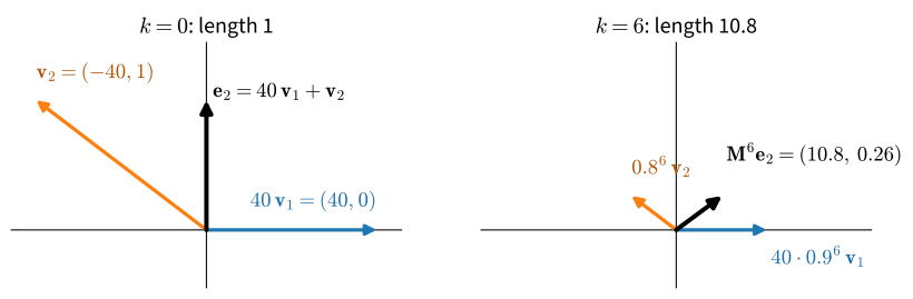
Its eigenvalues are its diagonal entries 0.9 and 0.8, both inside the unit circle, and they are distinct, so \(\mathbf M\) is diagonalizable. We find its eigenvectors and expand \(\mathbf e_2=(0,1)\) in them. For \(\lambda=0.9\), the second row of \(\mathbf M-0.9\mathbf I\) reads \(-0.1v_2=0\), so \(\mathbf v_1=(1,0)\). For \(\lambda=0.8\), the first row of \(\mathbf M-0.8\mathbf I\) reads \(0.1v_1+4v_2=0\), so \(\mathbf v_2=(-40,1)\). The two lines are \(\arctan(1/40)\approx1.4^\circ\) apart. The unit input is \(\mathbf e_2=40\mathbf v_1+\mathbf v_2\), and by Equation 33.3.4
\[ \mathbf M^k\mathbf e_2=40\cdot0.9^k\,\mathbf v_1+0.8^k\,\mathbf v_2 =\begin{pmatrix}40\,(0.9^k-0.8^k)\\0.8^k\end{pmatrix}. \tag{33.4.6}\]
A vector of length 1 is the difference of two components of length about 40. Both decay, but at different rates, so their difference first grows. The first entry \(40(0.9^k-0.8^k)\) peaks where its derivative in \(k\) vanishes, where \((9/8)^k=\ln0.8/\ln0.9\), at \(k\approx6.4\), with value about 10.8. Figure 33.4.3 draws the two components at \(k=0\) and \(k=6\). The bound Equation 33.4.4 with unit eigenvectors has \(\kappa_2(\mathbf V)=80\) and gives \(\|\mathbf M^6\|_2\le80\cdot0.9^6\approx42.5\). The bound holds, but it is four times the actual value 10.8.
The cell checks the derivation and compares \(\mathbf M\) with the diagonal matrix \(\boldsymbol\Lambda=\operatorname{diag}(0.9,0.8)\), which has the same eigenvalues and is normal.
M = np.array([[0.9, 4.0], [0.0, 0.8]])
Lam = np.diag([0.9, 0.8])                   # same eigenvalues, normal
lam, V = np.linalg.eig(M)                   # unit eigenvectors as columns
print('eigenvalues:', lam)
print('coefficients of e_2 on the unit eigenvectors:',
      np.linalg.solve(V, [0., 1.]))
ks = np.arange(61)
norm_M = [np.linalg.norm(np.linalg.matrix_power(M, k), 2) for k in ks]
norm_L = [np.linalg.norm(np.linalg.matrix_power(Lam, k), 2) for k in ks]
k_peak = int(np.argmax(norm_M))
print(f'max ||M^k|| = {norm_M[k_peak]:.3f} at k = {k_peak};  '
      f'max ||Lambda^k|| = {max(norm_L):.3f}')
print(f'kappa_2(V) = {np.linalg.cond(V):.1f}')
eigenvalues: [0.9 0.8]
coefficients of e_2 on the unit eigenvectors: [40. 40.01249805]
max ||M^k|| = 10.788 at k = 6; max ||Lambda^k|| = 1.000
kappa_2(V) = 80.0On the unit eigenvectors, \(\mathbf e_2\) has two coefficients of size about 40, the lengths of \(40\mathbf v_1\) and \(\mathbf v_2\). The largest \(\|\mathbf M^k\|_2\) is 10.8 at \(k=6\), while \(\boldsymbol\Lambda\) never exceeds its starting norm 1. With the same eigenvalues, the normal matrix contracts from the first step, while \(\mathbf M\) first grows ten-fold. Figure 33.4.4 (left) shows the two curves on a logarithmic scale; after the peak both fall with the same slope \(\log0.9\), as Gelfand’s formula requires.

33.4.2.4 Pseudospectra
This subsection adds a diagnostic, not a new phenomenon, and can be skipped. The eigenvalues of a matrix that is not normal are also sensitive to perturbations. The \(\varepsilon\)-pseudospectrum collects every number that becomes an eigenvalue under a perturbation \(\mathbf E\) of size at most \(\varepsilon\), and is computed from the resolvent \((z\mathbf I-\mathbf A)^{-1}\):
\[ \Lambda_\varepsilon(\mathbf A) =\{z\in\mathbb C:z\text{ is an eigenvalue of }\mathbf A+\mathbf E \text{ for some }\|\mathbf E\|_2\le\varepsilon\} =\{z\in\mathbb C:\|(z\mathbf I-\mathbf A)^{-1}\|_2\ge1/\varepsilon\}, \tag{33.4.7}\]
The resolvent norm counts as infinite at an eigenvalue; the equality of the two sets is Exercise 4. For a normal matrix the resolvent norm is the reciprocal of the distance from \(z\) to the nearest eigenvalue. For \(\mathbf M\) it is far larger, as the norms at \(z=1\), a point on the unit circle, show.
I = np.eye(2)
print(f'||(I - M)^-1||      = {np.linalg.norm(np.linalg.inv(I - M), 2):.1f}')
print(f'||(I - Lambda)^-1|| = {np.linalg.norm(np.linalg.inv(I - Lam), 2):.1f}')
||(I - M)^-1|| = 200.3
||(I - Lambda)^-1|| = 10.0For \(\boldsymbol\Lambda\) the norm is 10, the reciprocal of the distance 0.1 to the eigenvalue 0.9. For \(\mathbf M\) it is 200.3, so a perturbation of size \(1/200.3\approx0.005\) already puts an eigenvalue of \(\mathbf M\) on the unit circle, where \(\boldsymbol\Lambda\) needs 0.1 (right panel of Figure 33.4.4). Rounding errors act as such perturbations, so the computed eigenvalues of a strongly non-normal matrix may be inaccurate. Section 33.6 continues with the Kreiss matrix theorem.
33.4.2.5 Products of Jacobians
A recurrent network (Section 8.6) computes its hidden state as \(\mathbf h_t=\phi(\mathbf W\mathbf h_{t-1}+\cdots)\), with the same weights \(\mathbf W\) at every step, and backpropagation through time multiplies the per-step Jacobians \(\mathbf D_t=\partial\mathbf h_t/\partial\mathbf h_{t-1}\):
\[ \nabla_{\mathbf{h}_0}\mathcal{L} = \mathbf{D}_1^\top\mathbf{D}_2^\top\cdots\mathbf{D}_T^\top \,\nabla_{\mathbf{h}_T}\mathcal{L}. \]
The gradient that reaches the first state is the last one multiplied by \(T\) matrices. These matrices differ from step to step, because the nonlinearity \(\phi\) is evaluated at different points, so the theory of powers of one matrix does not apply. The spectral radii of the factors say nothing about the product. Take
\[ \mathbf D_1=\begin{pmatrix}0&2\\0&0\end{pmatrix}, \qquad \mathbf D_2=\begin{pmatrix}0&0\\2&0\end{pmatrix}, \qquad \mathbf D_2\mathbf D_1=\begin{pmatrix}0&0\\0&4\end{pmatrix}. \]
Both factors are nilpotent with \(\rho=0\), and their product has \(\rho=4\): \(\mathbf D_1\) moves the second coordinate into the first, doubled, and \(\mathbf D_2\) moves it back, doubled again.
Three quantities describe iterated linear maps. The spectral radius gives the asymptotic rate of the powers of one fixed map. The spectral norm bounds every finite product, \(\|\mathbf D_T\cdots\mathbf D_1\|_2\le\prod_t\|\mathbf D_t\|_2\), here \(4\le2\cdot2\). The top Lyapunov exponent
\[ \mu=\lim_{T\to\infty}\frac1T\log\|\mathbf D_T\cdots\mathbf D_1\mathbf x_0\| \]
gives the average growth rate per step of a long product of changing maps. For independent, identically distributed random factors the limit exists with probability one under mild conditions (Furstenberg and Kesten 1960).
A gradient that is multiplied by maps with \(\mu>0\) explodes, and one with \(\mu<0\) vanishes (Bengio et al. 1994; Pascanu et al. 2013). The standard remedies act on these quantities rather than on eigenvalues. Orthogonal initialization (Saxe et al. 2014) makes the initial weight matrix orthogonal, so a linear recurrence preserves the length of every vector, a stronger property than \(\rho=1\). Gradient clipping caps the norm of the gradient after it has been computed. Gates, as in LSTMs and GRUs, change the Jacobians themselves so that some directions pass through with factors close to 1 (Section 8.6.2.1).
33.4.2.6 Random Matrices at Initialization
How large are these quantities for the random weight matrices of an untrained network? Let \(\mathbf A\) be \(n\times n\) with independent standard Gaussian entries, the real Ginibre ensemble (Ginibre 1965). As \(n\to\infty\), the eigenvalues divided by \(\sqrt n\) fill the unit disc in the complex plane uniformly: this is the circular law, which Tao and Vu (2010) prove for independent, identically distributed entries of mean 0 and variance 1. The circular law describes where almost all eigenvalues are; it does not exclude a few outliers. That none escapes, so that \(\rho(\mathbf A)/\sqrt n\to1\) with probability one, is a separate theorem (Geman 1986). The spectral norm behaves differently: \(\|\mathbf A\|_2/\sqrt n\to2\) (Yin et al. 1988). This is the Marchenko–Pastur law of Section 33.3.2.4 at aspect ratio \(c=1\). The largest eigenvalue of \(\tfrac1n\mathbf A^\top\mathbf A\) tends to the upper edge \((1+\sqrt c)^2=4\), and \(\|\mathbf A\|_2^2\) is \(n\) times that eigenvalue. At \(n=1000\) both limits are close.
n = 1000
A = np.random.randn(n, n)
print(f'rho(A) / sqrt(n)       = {np.abs(np.linalg.eigvals(A)).max() / n ** 0.5:.3f}')
print(f'sigma_max(A) / sqrt(n) = {np.linalg.norm(A, 2) / n ** 0.5:.3f}')rho(A) / sqrt(n) = 1.030
sigma_max(A) / sqrt(n) = 1.990rho(A) / sqrt(n) = 1.021
sigma_max(A) / sqrt(n) = 1.975rho(A) / sqrt(n) = 1.021
sigma_max(A) / sqrt(n) = 1.998rho(A) / sqrt(n) = 1.022
sigma_max(A) / sqrt(n) = 1.991For large \(n\) the spectral radius is within a few percent of \(\sqrt n\) and the largest stretch close to \(2\sqrt n\): a random matrix stretches some vectors twice as much as its eigenvalues suggest. Initialization schemes divide random weights by \(\sqrt{\textrm{fan-in}}\) for a different reason: with entries of variance \(1/n\), \(\mathbb{E}\|\mathbf A\mathbf x\|^2=\|\mathbf x\|^2\) for every fixed \(\mathbf x\), so squared lengths are preserved on average. A spectral radius near 1 is a side effect, and by Section 33.4.2.5 it does not control a product of such matrices. In fact the product of independent factors with this scaling shrinks a typical vector, \(\mu<0\), even though every factor preserves squared length on average. The logarithm is concave, so for a unit vector the average of \(\log\|\mathbf A\mathbf x\|^2\) lies below the logarithm of the average of \(\|\mathbf A\mathbf x\|^2\), which is zero, and it is the logarithms that add along a product (Exercise 7).
The random matrix and \(\mathbf M\) make the same point: eigenvalues say little about the stretch in a finite number of steps. Nor do they exist for rectangular matrices. The singular values of Section 33.5 measure stretch directly, for every matrix.
33.4.3 Summary
Without a factorization, Gershgorin discs bound the eigenvalues from the entries, and power iteration finds the dominant one at the rate \(|\lambda_2/\lambda_1|\), as in PageRank. The spectral radius gives the long-run rate of the powers of one matrix and nothing more: a matrix that is not normal can grow before it decays, and the eigenvalues of the factors say nothing about a product of different matrices. There the spectral norm bounds every finite product, and the Lyapunov exponent gives the average rate. A Gaussian \(n\times n\) matrix shows the gap between the two at initialization: its spectral radius is close to \(\sqrt n\), its spectral norm close to \(2\sqrt n\).
33.4.4 Exercises
A defective limit. For \(\varepsilon\ge0\), let
\[ \mathbf{A}_\varepsilon=\begin{pmatrix}2&1\\\varepsilon&2\end{pmatrix}. \]
- Find the eigenvalues and eigenvectors of \(\mathbf{A}_\varepsilon\) for \(\varepsilon>0\) and for \(\varepsilon=0\). Which multiplicities differ at \(\varepsilon=0\)?
- Collect the unit eigenvectors of \(\mathbf{A}_\varepsilon\) in the columns of \(\mathbf{V}_\varepsilon\). How do the angle between them and the condition number \(\kappa_2(\mathbf{V}_\varepsilon)\) of Equation 33.4.4 behave as \(\varepsilon\to0\)? Show that \(\sqrt\varepsilon\,\kappa_2(\mathbf V_\varepsilon)\) tends to a constant as \(\varepsilon\to0\), and find it.
- By how much do the eigenvalues of \(\mathbf{A}_0\) move when its lower-left entry changes from \(0\) to \(\varepsilon=10^{-10}\)? Compare with the eigenvalues of the symmetric matrix \(2\mathbf{I}+\varepsilon\left(\begin{smallmatrix}0&1\\1&0\end{smallmatrix}\right)\). This is the smallest case of Exercise 4a.
Spectral radius and norms. The spectral radius bounds every power of a matrix from below, and for normal matrices it also bounds them from above.
- Show that \(\rho(\mathbf{A})\le\|\mathbf{A}^k\|_2^{1/k}\) for every square matrix \(\mathbf{A}\) and every \(k\ge1\).
- The chain Equation 33.4.3 uses two facts without proof. Show that \(\|\mathbf{U}\mathbf{X}\mathbf{U}^*\|_2=\|\mathbf{X}\|_2\) for every unitary \(\mathbf{U}\) and every square \(\mathbf{X}\), and that the spectral norm of a diagonal matrix is the largest modulus of its diagonal entries.
- Show that the converse of Equation 33.4.3 fails: find a \(3\times3\) matrix that is not normal but satisfies \(\|\mathbf{A}^k\|_2=\rho(\mathbf{A})^k\) for every \(k\ge1\).
- For a given \(t>0\), construct a diagonalizable \(2\times2\) matrix with spectral radius \(1/2\) and \(\|\mathbf{A}\|_2>t\).
[code] Power-iteration rates. Let \(\mathbf{S}\) be the matrix of Figure 33.4.2.
- By Equation 33.4.2, the misalignment between the iterate and \(\mathbf{v}_1\) decays at the rate \(|\lambda_2/\lambda_1|=1/3\). How many iterations reduce it by a factor of \(100\)?
- Let \(\mathbf{A}\) be symmetric with unit eigenvector \(\mathbf{v}_1\) for \(\lambda_1\), and let \(\mathbf{x}=\mathbf{v}_1+\delta\mathbf{u}\) for a unit vector \(\mathbf{u}\) orthogonal to \(\mathbf{v}_1\). Show that the Rayleigh quotient of Section 33.3.2.3 satisfies \(R(\mathbf{x})-\lambda_1=O(\delta^2)\), with no term linear in \(\delta\). At which rate does the Rayleigh quotient of the power iterates therefore approach \(\lambda_1\)? Where does the argument use that \(\mathbf A\) is symmetric?
- Repeat the experiment of Figure 33.4.2 for \(\left(\begin{smallmatrix}1&0.1\\0.1&1\end{smallmatrix}\right)\), which has the same eigenvectors as \(\mathbf S\) and the eigenvalues 1.1 and 0.9, from a random start. Plot the sine of the angle to \(\mathbf v_1\) and the error of the Rayleigh quotient on a logarithmic scale for 30 steps. Predict both slopes and the number of steps each error needs to shrink by a factor of 100, and explain why this matrix converges so much more slowly than \(\mathbf S\).
[code] Pseudospectra and transient growth. ● Let \(\mathbf{M}\) be the non-normal matrix Equation 33.4.5 and \(\boldsymbol\Lambda=\operatorname{diag}(0.9,0.8)\) the normal matrix with the same eigenvalues, as in Section 33.4.2.3.
Prove the equality of the two sets in Equation 33.4.7. First show that \(\|(z\mathbf I-\mathbf A)^{-1}\|_2=1/\sigma_{\min}(z\mathbf I-\mathbf A)\), where \(\sigma_{\min}(\mathbf X)=\min_{\|\mathbf x\|=1}\|\mathbf X\mathbf x\|\). For one inclusion, take unit vectors \(\mathbf u\), \(\mathbf v\) with \((z\mathbf{I}-\mathbf{A})\mathbf{v}=\sigma\mathbf{u}\), \(\sigma=\sigma_{\min}(z\mathbf I-\mathbf A)\), and show that \(z\) is an eigenvalue of \(\mathbf{A}+\sigma\mathbf{u}\mathbf{v}^*\). For the other, apply \((z\mathbf I-\mathbf A)\mathbf x=\mathbf E\mathbf x\) to an eigenvector \(\mathbf x\) of \(\mathbf A+\mathbf E\). Using the resolvent norms printed in Section 33.4.2.4, how large a perturbation makes \(z=1\) an eigenvalue of a perturbed \(\mathbf{M}\), and how large for \(\boldsymbol\Lambda\)?
Suppose that \(\|\mathbf{A}^k\|_2\le K_0\) for all \(k\ge0\). Show that for \(|z|>1\) the series \(\sum_{k\ge0}\mathbf{A}^k/z^{k+1}\) converges to \((z\mathbf{I}-\mathbf{A})^{-1}\), and conclude that
\[ \sup_{k\ge0}\|\mathbf{A}^k\|_2\;\ge\;K(\mathbf{A})=\sup_{|z|>1}\,(|z|-1)\,\|(z\mathbf{I}-\mathbf{A})^{-1}\|_2 . \]
The quantity \(K(\mathbf{A})\) is called the Kreiss constant. Restate the bound in terms of pseudospectra: if \(\Lambda_\varepsilon(\mathbf{A})\) contains a point at distance \(\delta\) outside the unit circle, how large must some power of \(\mathbf{A}\) be?
Evaluate \(K(\mathbf{M})\) numerically on a grid of points \(z\) with \(|z|>1\), and compare it with the largest \(\|\mathbf{M}^k\|_2\) printed in Section 33.4.2.3. Find \(K(\boldsymbol\Lambda)\) by hand.
[code] Shifted inverse iteration. ● Power iteration finds only the dominant eigenvalue. Inverse iteration with shift \(\mu\) runs power iteration with \((\mathbf{A}-\mu\mathbf{I})^{-1}\) instead, solving one linear system per step (Golub and Van Loan 1996). Parts (a) to (c) use the symmetric matrix
\[ \mathbf A_4=\begin{pmatrix}1&0.1&0.1&0.1\\0.1&3&0.2&0.3\\0.1&0.2&5&0.5\\0.1&0.3&0.5&9\end{pmatrix}, \]
whose Gershgorin centres are 1, 3, 5, 9 and whose eigenvalues are about 0.99, 2.97, 4.95, and 9.08.
- Show that \((\mathbf{A}-\mu\mathbf{I})^{-1}\) has the same eigenvectors as \(\mathbf{A}\), and find its eigenvalues. Which eigenpair of \(\mathbf{A}\) does inverse iteration find, and at which rate does it converge?
- Run inverse iteration on \(\mathbf A_4\) with each of the four disc centres as the shift. How many iterations does each run need until the sine of the angle between the iterate and the eigenvector returned by
np.linalg.eighfalls below \(10^{-10}\)? Compare with plain power iteration for the largest eigenvalue. - Rayleigh quotient iteration replaces the fixed shift by the Rayleigh quotient of the current iterate at every step. Repeat (b) with the disc centres as initial shifts. Relate the iteration counts to Exercise 3b.
- Run inverse iteration on the \(3\times3\) matrix Equation 33.4.1 with the real shift \(\mu=4\). Why does it never converge? Replace the shift by \(4+i\) (complex arithmetic) and explain the observed rate of about 0.02 per step from the distances \(|\lambda-\mu|\) of the three eigenvalues.
[code] Damping in PageRank. ● Let \(\mathbf{P}\) be a column-stochastic \(n\times n\) matrix and \(\mathbf{G}=\alpha\mathbf{P}+(1-\alpha)\tfrac1n\mathbf{1}\mathbf{1}^\top\) with \(0<\alpha<1\), the damped matrix of Section 33.4.1.3.
- Let \(\mathbf{P}\mathbf{x}=\lambda\mathbf{x}\). Show that \(\mathbf{1}^\top\mathbf{x}=0\) whenever \(\lambda\neq1\), and that \(\mathbf{G}\mathbf{x}=\alpha\lambda\mathbf{x}\) whenever \(\mathbf{1}^\top\mathbf{x}=0\).
- The eigenvalue \(1\) of \(\mathbf{P}\) can be repeated, as it is when the links split into disconnected pockets. You may use that every column-stochastic \(\mathbf P\) has a non-negative eigenvector for the eigenvalue 1 (a stationary distribution). Show that the vectors \(\mathbf{x}\) of this eigenspace with \(\mathbf{1}^\top\mathbf{x}=0\) form a subspace of dimension one less than the eigenspace. Conclude that for diagonalizable \(\mathbf{P}\) the eigenvalues of \(\mathbf{G}\) are \(1\) and \(\alpha\lambda_2(\mathbf{P}),\ldots,\alpha\lambda_n(\mathbf{P})\), which gives the bound \(|\lambda_2(\mathbf{G})|\le\alpha\) of Haveliwala and Kamvar (2003) .
- Four pages link in a cycle, \(1\to2\to3\to4\to1\). Find the eigenvalues of their link matrix \(\mathbf{P}\). Why does undamped power iteration started at page \(1\) never converge?
- With \(\alpha=0.85\) and the cycle of (c), run power iteration on \(\mathbf{G}\) from page \(1\), and count the iterations until the \(\ell_1\) distance to the stationary distribution falls below \(10^{-8}\). Compare with the prediction \(0.85^k\le10^{-8}\) from (b).
- Check numerically on the three-page example of Section 33.4.1.3 that the eigenvalues of \(\mathbf G\) are \(\alpha\) times those of \(\mathbf P\), apart from the eigenvalue 1, and that the stationary distribution moves from \((0.3,0.4,0.3)\) to about \((0.303,0.394,0.303)\). Why does damping move it toward uniform?
[code] Lyapunov exponents of random products. ●● Let \(\mathbf{D}_1,\mathbf{D}_2,\ldots\) be independent \(n\times n\) matrices with independent \(\mathcal{N}(0,1/n)\) entries, a linear model of the Jacobians of a deep network at fan-in initialization, and let \(\mathbf{x}_0\) be a unit vector. By Section 33.4.2.6, each factor has spectral radius close to \(1\) for large \(n\). Section 33.4.2.5 summarizes the growth of the product by its top Lyapunov exponent
\[ \mu=\lim_{T\to\infty}\frac1T\log\|\mathbf{D}_T\cdots\mathbf{D}_1\mathbf{x}_0\|, \]
which exists with probability one by the theorem of Furstenberg and Kesten.
Show that \(\mathbb{E}\|\mathbf{D}\mathbf{x}\|^2=\|\mathbf{x}\|^2\) for every fixed \(\mathbf{x}\), so that this scaling preserves squared norms on average.
Let \(\mathbf{u}_0=\mathbf{x}_0\) and \(\mathbf{u}_t=\mathbf{x}_t/\|\mathbf{x}_t\|\) for the iterates \(\mathbf{x}_t=\mathbf{D}_t\cdots\mathbf{D}_1\mathbf{x}_0\). Given \(\mathbf{D}_1,\ldots,\mathbf{D}_{t-1}\), what is the distribution of \(n\|\mathbf{D}_t\mathbf{u}_{t-1}\|^2\)? Use the answer to write \(\log\|\mathbf{D}_T\cdots\mathbf{D}_1\mathbf{x}_0\|\) as a sum of independent terms. With \(\mathbb{E}\log\chi^2_n=\psi(n/2)+\log2\), where \(\psi\) is the digamma function, derive the closed form of Cohen and Newman (1984)
\[ \mu=\tfrac12\bigl(\psi(n/2)+\log2-\log n\bigr). \]
Show that \(\mu<0\) for every \(n\), although (a) holds. Evaluate \(\mu\) in closed form for \(n=1\), using \(\psi(1/2)=-\gamma_{\textrm{E}}-2\log2\) with Euler’s constant \(\gamma_{\textrm{E}}\approx0.5772\). Using \(\psi(x)=\log x-\tfrac1{2x}+O(x^{-2})\), show that \(\mu\approx-1/(2n)\) for large \(n\).
Simulate \(T=10^4\) steps with renormalization for \(n\in\{1,2,5,50\}\), and compare the measured exponent with (b) and with the logarithms of the spectral radius and of the largest singular value of single factors. By which factor does a typical input shrink in a linear network of width \(50\) and depth \(100\) at this initialization? What does the comparison say about the three quantities of Section 33.4.2.5?