%matplotlib inline
from d2l import torch as d2l
import torch4.4 Numerical Stability and Initialization
Every model so far has required us to initialize its parameters from some chosen distribution, and we have taken those choices for granted. They are not innocuous. The initialization scheme interacts with the choice of activation function to determine whether gradients flow at a usable scale, or instead vanish (so learning stalls) or explode (so it diverges), and hence how fast optimization converges, or whether it converges at all. This section makes the failure modes concrete and develops the variance-preserving heuristics (Xavier and He initialization) that fix them.
%matplotlib inline
from d2l import tensorflow as d2l
import tensorflow as tf%matplotlib inline
from d2l import jax as d2l
import jax
from jax import numpy as jnp
from jax import grad, vmap%matplotlib inline
from d2l import mxnet as d2l
from mxnet import autograd, np, npx
npx.set_np()4.4.1 Vanishing and Exploding Gradients
Consider a deep network with \(L\) layers, input \(\mathbf{x}\) and output \(\mathbf{o}\). With each layer \(l\) defined by a transformation \(f_l\) parametrized by weights \(\mathbf{W}^{(l)}\), whose hidden layer output is \(\mathbf{h}^{(l)}\) (let \(\mathbf{h}^{(0)} = \mathbf{x}\)), our network can be expressed as:
\[\mathbf{h}^{(l)} = f_l (\mathbf{h}^{(l-1)}) \textrm{ and thus } \mathbf{o} = f_L \circ \cdots \circ f_1(\mathbf{x}). \tag{4.4.1}\]
If all the hidden layer output and the input are vectors, we can write the gradient of \(\mathbf{o}\) with respect to any set of parameters \(\mathbf{W}^{(l)}\) as follows:
\[\partial_{\mathbf{W}^{(l)}} \mathbf{o} = \underbrace{\partial_{\mathbf{h}^{(L-1)}} \mathbf{h}^{(L)}}_{ \mathbf{M}^{(L)} \stackrel{\textrm{def}}{=}} \cdots \underbrace{\partial_{\mathbf{h}^{(l)}} \mathbf{h}^{(l+1)}}_{ \mathbf{M}^{(l+1)} \stackrel{\textrm{def}}{=}} \underbrace{\partial_{\mathbf{W}^{(l)}} \mathbf{h}^{(l)}}_{ \mathbf{v}^{(l)} \stackrel{\textrm{def}}{=}}. \tag{4.4.2}\]
In other words, this gradient is the product of \(L-l\) matrices \(\mathbf{M}^{(L)} \cdots \mathbf{M}^{(l+1)}\) and the gradient operator \(\mathbf{v}^{(l)}\). Thus we are susceptible to the same problems of numerical underflow that often crop up when multiplying together too many probabilities. Products of probabilities can often be stabilized by switching to log-space, which represents multiplication as addition. Unfortunately, our problem above is more serious: each Jacobian \(\mathbf{M}^{(l)}\) can stretch or shrink the vectors it acts on by widely varying factors (its singular values: for the rectangular Jacobians that arise when layer widths differ, these are the right notion of “how much the matrix scales things”). A per-layer factor of \(\rho\) compounds to \(\rho^{\,L-l}\) across the product, so factors even modestly different from \(1\) make the overall gradient very large or very small geometrically fast; Section 24.2.5 develops the growth rate of such a product’s singular values.
The risks posed by unstable gradients go beyond numerical representation. Gradients of unpredictable magnitude also threaten the stability of our optimization algorithms. We may be facing parameter updates that are either (i) excessively large, destroying our model (the exploding gradient problem); or (ii) excessively small (the vanishing gradient problem), rendering learning impossible as parameters hardly move on each update.
4.4.1.1 Vanishing Gradients
One frequent culprit causing the vanishing gradient problem is the choice of the activation function \(\sigma\) that is appended following each layer’s linear operations. Historically, the sigmoid function \(1/(1 + \exp(-x))\) (introduced in Section 4.1) was popular because it resembles a thresholding function. Since early artificial neural networks were inspired by biological neural networks, the idea of neurons that fire either fully or not at all (like biological neurons) seemed appealing. Consider the sigmoid to see why it can cause vanishing gradients.
x = torch.arange(-8.0, 8.0, 0.1, requires_grad=True)
y = torch.sigmoid(x)
y.backward(torch.ones_like(x))

d2l.plot(x.detach().numpy(), [y.detach().numpy(), x.grad.numpy()],
         legend=['sigmoid', 'gradient'], figsize=(4.5, 2.5))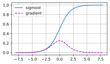
x = tf.Variable(tf.range(-8.0, 8.0, 0.1))
with tf.GradientTape() as t:
    y = tf.nn.sigmoid(x)
d2l.plot(x.numpy(), [y.numpy(), t.gradient(y, x).numpy()],
         legend=['sigmoid', 'gradient'], figsize=(4.5, 2.5))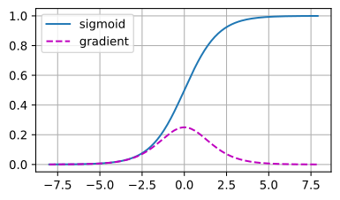
x = jnp.arange(-8.0, 8.0, 0.1)
y = jax.nn.sigmoid(x)
grad_sigmoid = vmap(grad(jax.nn.sigmoid))
d2l.plot(x, [y, grad_sigmoid(x)],
         legend=['sigmoid', 'gradient'], figsize=(4.5, 2.5))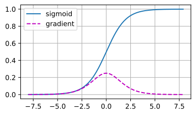
x = np.arange(-8.0, 8.0, 0.1)
x.attach_grad()
with autograd.record():
    y = npx.sigmoid(x)
y.backward()

d2l.plot(x, [y, x.grad], legend=['sigmoid', 'gradient'], figsize=(4.5, 2.5))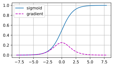
As you can see, the sigmoid’s gradient vanishes both when its inputs are large and when they are small. Moreover, the sigmoid’s derivative never exceeds \(0.25\) (its peak, attained at zero), so even in the Goldilocks zone, where the inputs to many of the sigmoids are close to zero, each sigmoid contributes a factor of at most \(1/4\), and with weights of unit scale ten sigmoid layers shrink the gradient by \(0.25^{10} \approx 10^{-6}\). Away from that zone the situation is far worse, and the gradients of the overall product vanish outright. When our network has many layers, unless we are careful, the gradient will likely be cut off at some layer. Indeed, this problem used to plague deep network training (Bengio et al. 1994). Consequently, ReLUs, which are more stable (but less neurally plausible), have emerged as the default choice for practitioners.
4.4.1.2 Exploding Gradients
The opposite problem, when gradients explode, can be similarly vexing. To illustrate this a bit better, we draw 100 Gaussian random matrices and multiply them with some initial matrix. For the scale that we picked (the choice of the variance \(\sigma^2=1\)), the matrix product explodes. When this happens because of the initialization of a deep network, we have no chance of getting a gradient descent optimizer to converge.
M = torch.normal(0, 1, size=(4, 4))
print('a single matrix \n',M)
for i in range(100):
    M = M @ torch.normal(0, 1, size=(4, 4))
print('after multiplying 100 matrices\n', M)
a single matrix
tensor([[-0.9753, -2.4309, -0.6217, -0.9488],
[ 0.5474, -0.3909, 1.7120, 0.4327],
[ 1.6211, -0.4342, 1.1437, -0.6168],
[-0.5642, -0.6920, 0.6003, 0.9131]])
after multiplying 100 matrices
tensor([[ 1.1962e+23, 1.0111e+23, 1.3713e+23, -2.7019e+23],
[ 7.4143e+21, 6.2674e+21, 8.4994e+21, -1.6747e+22],
[-1.2204e+23, -1.0316e+23, -1.3990e+23, 2.7565e+23],
[ 1.0273e+23, 8.6837e+22, 1.1777e+23, -2.3204e+23]])M = tf.random.normal((4, 4))
print('a single matrix \n', M)
for i in range(100):
M = tf.matmul(M, tf.random.normal((4, 4)))
print('after multiplying 100 matrices\n', M.numpy())a single matrix
tf.Tensor(
[[ 0.88569 -0.53551334 -2.0258462 -1.6222503 ]
[ 0.08253931 0.37377733 -1.1129707 0.7584501 ]
[-0.30639806 0.44809902 1.0800251 -0.8498218 ]
[-0.37185267 -1.3523052 0.4892188 -1.1749656 ]], shape=(4, 4), dtype=float32)
after multiplying 100 matrices
[[-3.3796842e+23 -1.4009740e+23 4.3313110e+23 7.5757996e+23]
[ 8.0702145e+22 3.3508249e+22 -1.0345620e+23 -1.8100430e+23]
[-1.6039657e+23 -6.6450585e+22 2.0551867e+23 3.5942717e+23]
[-7.8191073e+22 -3.2419027e+22 1.0021750e+23 1.7529337e+23]]M = jax.random.normal(d2l.get_key(), (4, 4))
print('a single matrix \n', M)
for i in range(100):
M = jnp.matmul(M, jax.random.normal(d2l.get_key(), (4, 4)))
print('after multiplying 100 matrices\n', M)a single matrix
[[-2.4424558 -2.0356805 0.20554423 -0.3535502 ]
[-0.76197404 -1.1785518 -1.1482196 0.29716578]
[-1.3105359 2.1302025 -0.18957235 0.9640122 ]
[-1.3011001 -0.7486938 -0.3729984 0.4427907 ]]
after multiplying 100 matrices
[[ 3.35693768e+22 1.62961708e+23 1.05114754e+23 -1.30175845e+23]
[ 3.68543113e+22 1.78908341e+23 1.15400786e+23 -1.42914213e+23]
[ 2.58828041e+22 1.25647169e+23 8.10458421e+22 -1.00368419e+23]
[ 3.11851576e+22 1.51387529e+23 9.76490918e+22 -1.20930216e+23]]M = np.random.normal(size=(4, 4))
print('a single matrix', M)
for i in range(100):
M = np.dot(M, np.random.normal(size=(4, 4)))
print('after multiplying 100 matrices', M)a single matrix [[ 0.21544254 -1.5842865 0.73179865 -0.6055198 ]
[-0.41833407 -0.09534191 -0.02739832 0.9578756 ]
[-0.60731924 0.97379816 -0.40570006 0.12149587]
[-0.1136004 0.49238634 -1.2923752 0.5174167 ]]
after multiplying 100 matrices [[ 6.1329105e+22 9.0935597e+21 3.0797470e+22 -2.1217980e+22]
[-5.3375046e+22 -7.9141739e+21 -2.6803193e+22 1.8466116e+22]
[-1.6772870e+22 -2.4869927e+21 -8.4227840e+21 5.8028943e+21]
[ 2.8053260e+21 4.1596003e+20 1.4087421e+21 -9.7055689e+20]]4.4.1.3 Breaking the Symmetry
Another problem in neural network design is the symmetry inherent in their parametrization. Assume that we have a simple MLP with one hidden layer and two units. In this case, we could permute the weights \(\mathbf{W}^{(1)}\) of the first layer and likewise permute the weights of the output layer to obtain the same function. There is nothing special differentiating the first and second hidden units. In other words, we have permutation symmetry among the hidden units of each layer.
This symmetry directly restricts learning. Consider the aforementioned one-hidden-layer MLP with two hidden units. For illustration, suppose that the output layer transforms the two hidden units into only one output unit. Suppose we initialized all the parameters of the hidden layer as \(\mathbf{W}^{(1)} = c\) for some constant \(c\). In this case, during forward propagation either hidden unit takes the same inputs and parameters producing the same activation which is fed to the output unit. During backpropagation, differentiating the output unit with respect to parameters \(\mathbf{W}^{(1)}\) gives a gradient all of whose elements take the same value. Thus, after gradient-based iteration (e.g., minibatch stochastic gradient descent), all the elements of \(\mathbf{W}^{(1)}\) still take the same value. Such iterations would never break the symmetry on their own and we might never be able to realize the network’s expressive power. The hidden layer would behave as if it had only a single unit. Note that while minibatch stochastic gradient descent would not break this symmetry, dropout regularization (Section 4.6) would!
4.4.2 Parameter Initialization
One way of addressing (or at least mitigating) the issues raised above is through careful initialization. As we will see later, additional care during optimization and suitable regularization can further enhance stability.
4.4.2.1 Default Initialization
In the previous sections, e.g., in Section 2.5, we initialized weights by drawing them from a normal distribution with a small, fixed standard deviation. If we do not specify an initialization method at all, the library falls back to its own default scheme. These defaults differ across libraries and layer types: some scale with fan-in, while others use a fixed range. They are conveniences rather than a portable mathematical guarantee. For an experiment whose initialization matters, choose a named initializer explicitly and record its parameters. Defaults often work well for moderately sized networks, but they become unreliable as depth grows. The variance analysis that follows explains why they work, where they break, and what to reach for instead.
4.4.2.2 Xavier Initialization
We inspect the scale distribution of an output \(o_{i}\) for some fully connected layer without nonlinearities. With \(n_\textrm{in}\) inputs \(x_j\) and their associated weights \(w_{ij}\) for this layer, an output is given by
\[o_{i} = \sum_{j=1}^{n_\textrm{in}} w_{ij} x_j.\]
The weights \(w_{ij}\) are all drawn independently from the same distribution. Furthermore, let’s assume that this distribution has zero mean and variance \(\sigma^2\). Note that this does not mean that the distribution has to be Gaussian, only that its mean and variance must exist. Assume also that the inputs to the layer \(x_j\) also have zero mean and variance \(\gamma^2\) and that they are independent of \(w_{ij}\) and independent of each other. In this case, we can compute the mean of \(o_i\):
\[ \begin{aligned} E[o_i] & = \sum_{j=1}^{n_\textrm{in}} E[w_{ij} x_j] \\&= \sum_{j=1}^{n_\textrm{in}} E[w_{ij}] E[x_j] \\&= 0, \end{aligned}\]
and the variance:
\[ \begin{aligned} \textrm{Var}[o_i] & = E[o_i^2] - (E[o_i])^2 \\ & = \sum_{j=1}^{n_\textrm{in}} E[w^2_{ij} x^2_j] - 0 \\ & = \sum_{j=1}^{n_\textrm{in}} E[w^2_{ij}] E[x^2_j] \\ & = n_\textrm{in} \sigma^2 \gamma^2. \end{aligned} \]
Here we used \(E[w_{ij}^2] = \textrm{Var}[w_{ij}] = \sigma^2\), which holds because the weights have zero mean (\(\textrm{Var}[w] = E[w^2] - E[w]^2 = E[w^2]\)), and likewise \(E[x_j^2] = \gamma^2\). In the second line, expanding the square of the sum also produces cross terms \(E[w_{ij} w_{ik} x_j x_k]\) for \(j \neq k\); these vanish because the weights are independent of each other (and of the inputs) and have zero mean.
One way to keep the variance fixed is to set \(n_\textrm{in} \sigma^2 = 1\). Next consider backpropagation. A gradient signal flowing back through this layer is multiplied by \(\mathbf{W}^\top\), so by the identical variance computation, now summing over the \(n_\textrm{out}\) outputs the layer feeds, its variance is scaled by \(n_\textrm{out} \sigma^2\). Keeping the backward signal’s variance fixed therefore requires \(n_\textrm{out} \sigma^2 = 1\), where \(n_\textrm{out}\) is the number of outputs of this layer. This leaves us in a dilemma: we cannot satisfy both conditions simultaneously unless \(n_\textrm{in}=n_\textrm{out}\). A compromise satisfies the averaged condition
\[ \begin{aligned} \frac{1}{2} (n_\textrm{in} + n_\textrm{out}) \sigma^2 = 1 \textrm{ or equivalently } \sigma = \sqrt{\frac{2}{n_\textrm{in} + n_\textrm{out}}}. \end{aligned} \]
This variance argument yields Xavier initialization, named after the first author of its creators (Glorot and Bengio 2010). Typically, the Xavier initialization samples weights from a Gaussian distribution with zero mean and variance \(\sigma^2 = \frac{2}{n_\textrm{in} + n_\textrm{out}}\). We can also adapt this to choose the variance when sampling weights from a uniform distribution. Note that the uniform distribution \(U(-a, a)\) has variance \(\frac{a^2}{3}\). Plugging \(\frac{a^2}{3}\) into our condition on \(\sigma^2\) prompts us to initialize according to
\[U\left(-\sqrt{\frac{6}{n_\textrm{in} + n_\textrm{out}}}, \sqrt{\frac{6}{n_\textrm{in} + n_\textrm{out}}}\right). \tag{4.4.3}\]
Though the assumption that there are no nonlinearities in the above mathematical reasoning can be easily violated in neural networks, Xavier initialization often works well in practice.
4.4.2.3 He Initialization
The Xavier analysis above assumed a layer without nonlinearities. The argument breaks in a specific, fixable way once we insert a ReLU. First, note what the variance computation above actually consumed. With independent zero-mean weights, \(E[o_i] = 0\), and \(E[o_i^2] = n_\textrm{in} \sigma^2 E[x_j^2]\) depends on the inputs only through their second moment \(E[x_j^2]\). So we must track the second moment through the nonlinearity. Recall that \(\textrm{ReLU}(z) = \max(0, z)\) zeroes every negative pre-activation and passes every positive one through unchanged. If the pre-activations are symmetric about zero, as they are when the weights have a symmetric distribution independent of the inputs, then \(\textrm{ReLU}(z)^2\) equals \(z^2\) on the positive half of the distribution and equals \(0\) on the negative half, so the rectifier halves the second moment: \(E[\textrm{ReLU}(z)^2] = \tfrac{1}{2}E[z^2]\). (Its effect on the variance is messier, because \(\textrm{ReLU}(z)\) is no longer zero-mean, as the exercises explore.)
Let \(q=E[h_j^2]\) be the second moment entering a linear layer. Its preactivation has second moment \(n_\textrm{in}\sigma^2q\), and the following ReLU produces \(q' = \tfrac{1}{2}n_\textrm{in}\sigma^2q\) under the symmetry and independence assumptions above. To keep this second moment fixed across layers we must compensate by doubling the weight variance:
\[\sigma^2 = \frac{2}{n_\textrm{in}}. \tag{4.4.4}\]
This is He (or Kaiming) initialization (He et al. 2015), and it is the standard choice for the ReLU-family activations this chapter uses throughout. Because Xavier and He differ only by this factor of two and by which fan size they key on, they are easy to confuse; the rule of thumb is Xavier for \(\tanh\) and sigmoid, He for ReLU. Most libraries ship both as named initializers, and we return to invoking them through the parameter-initialization API in Chapter 5.
4.4.2.4 Watching the Variance Propagate
The preceding matrix product demonstrated growth under an unsuitable scale. The following experiment compares three initialization regimes: push a unit-scale signal through \(50\) ReLU layers of width \(100\) and track the second moment \(E[(h^{(l)})^2]\) of the activations (the quantity the He argument preserves) layer by layer, under three weight scales: the naive \(\mathcal{N}(0,1)\), Xavier, and He. To avoid floating-point overflow along the way, we renormalize the activations after each layer and accumulate the per-layer gains instead; because ReLU is positively homogeneous (\(\operatorname{ReLU}(a\mathbf{x}) = a\operatorname{ReLU}(\mathbf{x})\) for \(a > 0\)), this rescaling is exact, not an approximation.
depth, width = 50, 100
scales = {'N(0, 1)': 1.0, 'Xavier': (2 / (width + width)) ** 0.5,
          'He': (2 / width) ** 0.5}
curves = []
for scale in scales.values():
    h, m, curve = torch.randn(1000, width), 1.0, []
    for _ in range(depth):
        h = torch.relu(h @ (scale * torch.randn(width, width)))
        gain = float((h ** 2).mean())  # this layer's factor on E[h^2]
        m *= gain
        curve.append(m)
        h = h / gain ** 0.5  # renormalize: exact, since ReLU is homogeneous
    curves.append(curve)
d2l.plot(list(range(1, depth + 1)), curves, 'layer', 'second moment of h',
         legend=list(scales), yscale='log')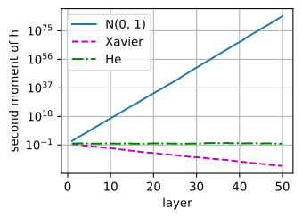
depth, width = 50, 100
scales = {'N(0, 1)': 1.0, 'Xavier': (2 / (width + width)) ** 0.5,
          'He': (2 / width) ** 0.5}
curves = []
for scale in scales.values():
    h, m, curve = tf.random.normal((1000, width)), 1.0, []
    for _ in range(depth):
        h = tf.nn.relu(tf.matmul(h, scale * tf.random.normal(
            (width, width))))
        gain = float(tf.reduce_mean(h ** 2))  # factor on E[h^2]
        m *= gain
        curve.append(m)
        h = h / gain ** 0.5  # renormalize: exact, since ReLU is homogeneous
    curves.append(curve)
d2l.plot(list(range(1, depth + 1)), curves, 'layer', 'second moment of h',
         legend=list(scales), yscale='log')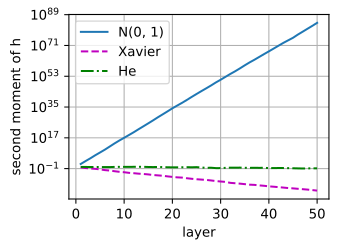
depth, width = 50, 100
scales = {'N(0, 1)': 1.0, 'Xavier': (2 / (width + width)) ** 0.5,
          'He': (2 / width) ** 0.5}
curves = []
for scale in scales.values():
    h, m, curve = jax.random.normal(d2l.get_key(), (1000, width)), 1.0, []
    for _ in range(depth):
        h = jax.nn.relu(h @ (scale * jax.random.normal(
            d2l.get_key(), (width, width))))
        gain = float((h ** 2).mean())  # this layer's factor on E[h^2]
        m *= gain
        curve.append(m)
        h = h / gain ** 0.5  # renormalize: exact, since ReLU is homogeneous
    curves.append(curve)
d2l.plot(list(range(1, depth + 1)), curves, 'layer', 'second moment of h',
         legend=list(scales), yscale='log')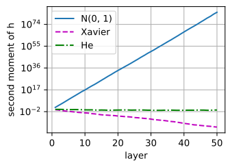
depth, width = 50, 100
scales = {'N(0, 1)': 1.0, 'Xavier': (2 / (width + width)) ** 0.5,
          'He': (2 / width) ** 0.5}
curves = []
for scale in scales.values():
    h, m, curve = np.random.normal(size=(1000, width)), 1.0, []
    for _ in range(depth):
        h = npx.relu(np.dot(h, scale * np.random.normal(
            size=(width, width))))
        gain = float((h ** 2).mean())  # this layer's factor on E[h^2]
        m *= gain
        curve.append(m)
        h = h / gain ** 0.5  # renormalize: exact, since ReLU is homogeneous
    curves.append(curve)
d2l.plot(list(range(1, depth + 1)), curves, 'layer', 'second moment of h',
         legend=list(scales), yscale='log')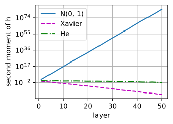
This finite-width realization displays the three regimes predicted by the second-moment calculation. Under \(\mathcal{N}(0,1)\) weights the expected gain is \(n_\textrm{in}/2=50\) per layer. For Xavier weights followed by ReLU it is \(1/2\), whereas for He weights it is \(1\). The plotted trajectories fluctuate around those expectation-level factors; repeated seeds would reveal their dispersion. A related backward calculation gives the same scaling under additional mean-field independence assumptions. Both are initialization-time approximations, not exact statements about gradients during training. The exercises repeat the sweep without ReLU.
4.4.2.5 Scope of the Initialization Rules
Xavier and He initialization assume independent weights and simple feedforward layers at initialization. Shared parameters, recurrent dynamics, attention, and very deep compositions violate parts of that analysis. Later chapters introduce normalization layers (Section 7.3) and residual connections (Section 7.4), which provide additional paths for controlling signal scale. Specialized initializers remain useful when those architectural assumptions differ.
4.4.3 Summary
Vanishing and exploding gradients are common issues in deep networks. Great care in parameter initialization is required to ensure that gradients and parameters remain well controlled. Initialization heuristics are needed to ensure that the initial gradients are neither too large nor too small. Random initialization is key to ensuring that symmetry is broken before optimization. Xavier initialization keeps the variance of activations and gradients roughly constant across layers by scaling weights according to the number of inputs and outputs. For ReLU networks, He initialization scales the weight variance to \(2/n_\textrm{in}\) to compensate for the rectifier halving the activations’ second moment. ReLU activation functions mitigate the vanishing gradient problem. This can accelerate convergence.
4.4.4 Exercises
Other symmetries. Permuting the hidden units is not the only change of parameters that leaves an MLP’s function unchanged. Consider a one-hidden-layer MLP in which hidden unit \(j\) has incoming weights \(\mathbf{w}_j\), bias \(b_j\), and outgoing weights \(\mathbf{v}_j\).
- Prove that \(\textrm{ReLU}(\alpha z) = \alpha\, \textrm{ReLU}(z)\) for \(\alpha > 0\). Use this identity to show that replacing \((\mathbf{w}_j, b_j, \mathbf{v}_j)\) by \((\alpha \mathbf{w}_j, \alpha b_j, \mathbf{v}_j / \alpha)\) leaves the function of a ReLU network unchanged.
- Find a transformation of the parameters of a single hidden unit that leaves the function of a \(\tanh\) network unchanged.
- Identical hidden units are a fixed point of the permutation, and gradient descent started at that fixed point stays there. Find the parameters of a unit that the transformation of the previous part leaves unchanged. Then show that if all weights and biases of a \(\tanh\) network are initialized to zero, gradient descent changes only the output bias, at every step.
Adapted from Simon Prince, Understanding Deep Learning, Problems 3.5, 4.3, and 7.15.
Constant initialization. Initialize all weights of linear regression, and separately of softmax regression, to the same constant \(c\), and all biases to zero.
- For each model, write the gradient of the minibatch loss with respect to each weight at this initialization.
- Which weights, if any, receive identical gradients? Does the symmetry-breaking failure that this section describes for hidden units occur in either model?
Fan-in versus averaged fans. Following He et al. (2015), consider a linear network with \(L\) layers in which layer \(l\) maps \(n_{l-1}\) inputs to \(n_l\) outputs and draws its weights with variance \(\sigma_l^2\). By the computation of Section 4.4.2.2, layer \(l\) multiplies the second moment of the forward signal by \(n_{l-1}\sigma_l^2\) and that of the backward signal by \(n_l\sigma_l^2\).
- Set \(\sigma_l^2 = 1/n_{l-1}\) in every layer. Show that the forward second moment is preserved and that the backward second moment changes by the total factor \(n_L / n_0\), whatever the depth.
- Let the widths alternate as \(100, 400, 100, 400, \ldots\), and use Xavier initialization in every layer. Compute the factor by which one \(100 \to 400 \to 100\) pair of layers multiplies the forward second moment, and the factor after 50 such pairs.
- Which of the two rules keeps both second moments within a depth-independent factor of their initial values for every sequence of widths?
Variance under ReLU. ● The derivation in Section 4.4.2.3 tracks the second moment \(E[\textrm{ReLU}(z)^2]\) rather than the variance, because the next layer’s pre-activation \(o = \sum_j w_j h_j\) with independent zero-mean weights has \(\textrm{Var}[o] = n_\textrm{in}\sigma^2 E[h_j^2]\) whatever the mean of \(h_j\).
- For \(z \sim \mathcal{N}(0, \tau^2)\), compute \(E[\textrm{ReLU}(z)]\) and \(\textrm{Var}[\textrm{ReLU}(z)]\) explicitly, and show that the variance equals \(\left(\tfrac{1}{2} - \tfrac{1}{2\pi}\right)\tau^2\) rather than \(\tfrac{1}{2}\tau^2\).
- A tempting shortcut substitutes \(\textrm{Var}[h_j]\) for \(E[h_j^2]\) in the Xavier computation. Show that this shortcut prescribes \(\sigma^2 = 2 / \bigl(n_\textrm{in}(1 - 1/\pi)\bigr)\) instead of \(2/n_\textrm{in}\). Compute the factor by which each ReLU layer initialized this way actually multiplies the second moment, and the total factor over the 50 layers of the sweep in Section 4.4.2.4.
[code] Linear depth sweep. Rerun the depth-sweep experiment of Section 4.4.2.4 with the ReLU removed, i.e., for a purely linear stack of 50 layers of width 100 under the same three initialization schemes.
- For a linear layer with \(n_\textrm{in} = n_\textrm{out} = 100\), compute the expected per-layer factor \(n_\textrm{in}\sigma^2\) on the second moment under each of the three weight scales, and check the three factors against the slopes of the plotted curves.
- Compare the ranking of the three schemes with the ranking in the ReLU sweep and explain the difference.
[code] Tanh depth sweep. ● Rerun the depth-sweep experiment of Section 4.4.2.4 with \(\tanh\) in place of ReLU and with Xavier weights. A layer then maps the second moment \(q\) of its input to \(q' = E[\tanh(z)^2]\), where \(z\) is approximately \(\mathcal{N}(0, q)\).
- Use \(\tanh(z)^2 \approx z^2 - \tfrac{2}{3}z^4\) for small \(z\) to show that \(q' \approx q - 2q^2\). Over many layers, does the second moment stay constant, decay geometrically, or decay more slowly?
- Check the prediction by running the sweep without the renormalization step, and explain why that step is exact for ReLU but not for \(\tanh\).
Spectral norm bounds. The gradient in Equation 4.4.2 is a product of \(L - l\) Jacobians. The spectral norm (the largest singular value) is submultiplicative: \(\|\mathbf{A}\mathbf{B}\|_2 \le \|\mathbf{A}\|_2 \|\mathbf{B}\|_2\).
- Prove submultiplicativity from the definition \(\|\mathbf{A}\|_2 = \max_{\mathbf{x} \neq 0} \|\mathbf{A}\mathbf{x}\| / \|\mathbf{x}\|\).
- Use it to bound the norm of the gradient product in terms of the per-layer norms \(\|\mathbf{M}^{(l)}\|_2\). Which condition on the per-layer norms keeps this bound from growing geometrically with depth?
- This bound is only an upper bound. Explain why the condition of the previous part rules out exploding gradients but not vanishing ones, and give two \(2 \times 2\) matrices that satisfy the condition with equality but whose product has spectral norm strictly smaller than one.
[code] Layerwise adaptive scaling. ● Write \(\mathbf{g}^{(l)} = \nabla_{\mathbf{W}^{(l)}} J\) for the gradient of the loss \(J\) with respect to the weights of layer \(l\). Layerwise adaptive rate scaling (You et al. 2017) replaces the SGD update \(\mathbf{W}^{(l)} \leftarrow \mathbf{W}^{(l)} - \eta\, \mathbf{g}^{(l)}\) by
\[\mathbf{W}^{(l)} \leftarrow \mathbf{W}^{(l)} - \eta \, \frac{\|\mathbf{W}^{(l)}\|}{\|\mathbf{g}^{(l)}\|} \, \mathbf{g}^{(l)}, \tag{4.4.5}\]
where \(\|\cdot\|\) is the Frobenius norm. The scaled update has norm \(\eta\, \|\mathbf{W}^{(l)}\|\): every layer moves by the same fraction \(\eta\) of its weight norm, however large or small its raw gradient. An exploding gradient therefore changes only the direction of the update, not its size.
- Build a three-layer linear network of width 100 with \(\mathcal{N}(0, 1)\) weights. Draw one fixed batch of 256 inputs and 256 targets in \(\mathbb{R}^{100}\) from \(\mathcal{N}(0, \mathbf{I})\), and let \(J\) be the mean squared error over this batch. Train with plain SGD at \(\eta = 0.1\), record \(J\) and \(\|\mathbf{g}^{(1)}\|\) over the first ten steps, and show that both diverge.
- Replace the update by the scaled one, with the same \(\eta\), and repeat the ten steps. Does the loss decrease? Relate the outcome to the forward-pass scale of the network at this initialization.