%matplotlib inline
from d2l import torch as d2l
from safetensors.torch import load_file
import tiktoken
from tiktoken.load import data_gym_to_mergeable_bpe_ranks
import torch
from torch import nn
from torch.nn import functional as F11.2 A GPT from Scratch
A GPT-style language model adds token embeddings, positional information, a causal mask, and an output head to a stack of transformer blocks. We implement these components in a GPT class whose constructor includes the block options from Section 11.1 and a choice of positional scheme. With a current configuration, this class trains from scratch on The Time Machine in about a minute. With the GPT-2 configuration, it also accepts the released GPT-2 weights (Radford et al. 2019). These experiments illustrate how to interpret a loss curve, diagnose a poor normalization choice, and sample from a trained distribution.
%matplotlib inline
from d2l import jax as d2l
from flax import nnx
import jax
from jax import numpy as jnp
import optax
from safetensors import numpy as safetensors_numpy
import tiktoken
from tiktoken.load import data_gym_to_mergeable_bpe_ranks
11.2.1 From Blocks to a Language Model
Four ingredients turn a stack of transformer blocks into a GPT-style language model.
A token embedding and a tied head. A lookup table maps token ids into the residual stream; after the final block (and one last normalization, pre-norm convention), the same table, transposed, maps the stream back to logits over the vocabulary. Tying the two matrices saves a \(\textrm{vocab} \times d\) parameter block and consistently helps at small scale (Press and Wolf 2017); GPT-2 ties them too, which will spare us a tensor when we load its weights.
A causal mask. A language model predicts token \(t+1\) from tokens \(1,
\ldots, t\), so position \(t\) must not attend forward. In Section 11.1 we enforced causality by passing d2l.MultiHeadAttention a per-query valid length. Here we build the causal variant natively, for two reasons. First, efficiency: the fused attention kernels of Section 10.5 (scaled_dot_product_attention in PyTorch, dot_product_attention in JAX) take the causal mask as a flag and never materialize the \(n \times n\) score matrix. Second, positions.
Positions, inside attention or outside. The pos argument selects between the two schemes that Section 10.4 found in deployed models: 'learned' adds a trained position vector to the embedding — GPT-2’s scheme, capped at the table’s length — and 'rope' rotates queries and keys inside every attention head. RoPE is used by the Llama and Qwen model families cited later in this chapter. It lives where queries and keys are made, so the attention module implements it itself (the same _rope we gave TinyCharLM); nothing else in the model knows positions exist.
The blocks themselves are d2l.TransformerBlock, unchanged: the causal attention enters through the attn_factory hook.
class GPT(nn.Module):
    """Decoder-only transformer language model built from configurable
    blocks."""

    class CausalAttention(nn.Module):
        """Multi-head causal self-attention, optionally rotary."""
        def __init__(self, num_hiddens, num_heads, bias=False, rope=False):
            super().__init__()
            self.num_heads, self.rope = num_heads, rope
            self.W_qkv = nn.Linear(num_hiddens, 3 * num_hiddens, bias=bias)
            self.W_o = nn.Linear(num_hiddens, num_hiddens, bias=bias)

        def _rope(self, x):
            d = x.shape[-1]
            pos = torch.arange(x.shape[-2], dtype=torch.float32,
                               device=x.device)
            inv_freq = 10000.0 ** (
                -torch.arange(0, d, 2, device=x.device) / d)
            theta = pos[:, None] * inv_freq[None, :]
            cos, sin = torch.cos(theta), torch.sin(theta)
            x1, x2 = x[..., 0::2], x[..., 1::2]
            return torch.stack([x1 * cos - x2 * sin,
                                x1 * sin + x2 * cos], -1).flatten(-2)

        def forward(self, X, *_):
            B, T, D = X.shape
            q, k, v = self.W_qkv(X).chunk(3, -1)
            q, k, v = (u.reshape(B, T, self.num_heads, -1).transpose(1, 2)
                       for u in (q, k, v))
            if self.rope:
                q, k = self._rope(q), self._rope(k)
            Y = F.scaled_dot_product_attention(q, k, v, is_causal=True)
            return self.W_o(Y.transpose(1, 2).reshape(B, T, D))

    def __init__(self, vocab_size, num_hiddens=256, num_heads=8, num_blks=6,
                 max_len=1024, pos='rope', norm='rms', act='swiglu',
                 pre_norm=True, bias=False, dropout=0):
        super().__init__()
        self.pos, self.max_len = pos, max_len
        self.token_emb = nn.Embedding(vocab_size, num_hiddens)
        nn.init.normal_(self.token_emb.weight, std=0.02)
        if pos == 'learned':
            self.pos_emb = nn.Embedding(max_len, num_hiddens)
            nn.init.normal_(self.pos_emb.weight, std=0.02)
        attn = lambda: self.CausalAttention(num_hiddens, num_heads, bias,
                                            rope=(pos == 'rope'))
        self.blks = nn.ModuleList([
            d2l.TransformerBlock(num_hiddens, num_heads, dropout, norm, act,
                                 pre_norm, bias, attn_factory=attn)
            for _ in range(num_blks)])
        self.norm = (nn.RMSNorm if norm == 'rms'
                     else nn.LayerNorm)(num_hiddens)

    def forward(self, X):
        H = self.token_emb(X)
        if self.pos == 'learned':
            H = H + self.pos_emb(torch.arange(X.shape[1], device=X.device))
        for blk in self.blks:
            H = blk(H)
        return F.linear(self.norm(H), self.token_emb.weight)
class GPT(nnx.Module):
"""Decoder-only transformer language model built from configurable
blocks."""
class CausalAttention(nnx.Module):
"""Multi-head causal self-attention, optionally rotary."""
def __init__(self, num_hiddens, num_heads, bias=False, rope=False,
rngs=None):
rngs = nnx.Rngs(0) if rngs is None else rngs
self.num_heads, self.rope = num_heads, rope
self.W_qkv = nnx.Linear(num_hiddens, 3 * num_hiddens,
use_bias=bias, rngs=rngs)
self.W_o = nnx.Linear(num_hiddens, num_hiddens, use_bias=bias,
rngs=rngs)
def _rope(self, x):
# x: (batch, num_steps, num_heads, head_dim)
d = x.shape[-1]
pos = jnp.arange(x.shape[1], dtype=jnp.float32)
inv_freq = 10000.0 ** (-jnp.arange(0, d, 2) / d)
theta = pos[:, None] * inv_freq[None, :]
cos = jnp.cos(theta)[:, None, :] # broadcast over heads
sin = jnp.sin(theta)[:, None, :]
x1, x2 = x[..., 0::2], x[..., 1::2]
return jnp.stack([x1 * cos - x2 * sin,
x1 * sin + x2 * cos], -1).reshape(x.shape)
def __call__(self, X, *_):
B, T, D = X.shape
q, k, v = jnp.split(self.W_qkv(X), 3, axis=-1)
q, k, v = (u.reshape(B, T, self.num_heads, -1)
for u in (q, k, v))
if self.rope:
q, k = self._rope(q), self._rope(k)
Y = jax.nn.dot_product_attention(q, k, v, is_causal=True)
return self.W_o(Y.reshape(B, T, D)), None
def __init__(self, vocab_size, num_hiddens=256, num_heads=8, num_blks=6,
max_len=1024, pos='rope', norm='rms', act='swiglu',
pre_norm=True, bias=False, dropout=0, rngs=None):
rngs = nnx.Rngs(0) if rngs is None else rngs
self.pos, self.max_len = pos, max_len
init = nnx.initializers.normal(0.02)
self.token_emb = nnx.Embed(vocab_size, num_hiddens,
embedding_init=init, rngs=rngs)
if pos == 'learned':
self.pos_emb = nnx.Embed(max_len, num_hiddens,
embedding_init=init, rngs=rngs)
attn = lambda rngs: self.CausalAttention(
num_hiddens, num_heads, bias, rope=(pos == 'rope'), rngs=rngs)
self.blks = nnx.List([
d2l.TransformerBlock(num_hiddens, num_heads, dropout, norm, act,
pre_norm, bias, attn_factory=attn,
rngs=rngs)
for _ in range(num_blks)])
self.norm = (nnx.RMSNorm if norm == 'rms'
else nnx.LayerNorm)(num_hiddens, rngs=rngs)
def __call__(self, X):
H = self.token_emb(X)
if self.pos == 'learned':
H = H + self.pos_emb(jnp.arange(X.shape[1]))
for blk in self.blks:
H = blk(H)
return self.token_emb.attend(self.norm(H))A shape check, and the census of the default configuration:
model = GPT(vocab_size=28)
X = torch.zeros(2, 16, dtype=torch.long)
d2l.check_shape(model(X), (2, 16, 28))
print(f'{sum(p.numel() for p in model.parameters()) / 1e6:.2f}M parameters')
4.73M parametersmodel = GPT(vocab_size=28)
X = jnp.zeros((2, 16), dtype=jnp.int32)
d2l.check_shape(model(X), (2, 16, 28))
n = sum(p.size for p in jax.tree.leaves(nnx.state(model, nnx.Param)))
print(f'{n / 1e6:.2f}M parameters')4.73M parametersThe model reads characters rather than subwords because the training corpus is small. Deployed language models tokenize into subwords — byte-pair encoding is the most common scheme — and Section 8.2 built a full BPE tokenizer; we will even reuse its GPT-2 pattern verbatim when we load GPT-2 below. BPE becomes advantageous on much larger corpora. On a 180 KB novel, a subword vocabulary would leave each token type a handful of training examples. Characters keep the statistics dense, the vocabulary trivial, and the comparison fair against the character-level models of previous chapters.
11.2.2 Training a Pre-Norm RMSNorm Configuration
We train the default configuration on the character-level Time Machine corpus. Its pre-norm, RMSNorm, SwiGLU, and RoPE settings also appear in the Llama and Qwen families (Touvron et al. 2023a). We set dropout=0.1 for this small repeated corpus. Several large-model reports tabulated later use no dropout, but this comparison does not isolate why. We record validation loss throughout training.
data = d2l.TimeMachine(batch_size=64, num_steps=128, tokenization='char',
                       num_train=100000, num_val=3000)

def val_loss(model, data):
    """Mean per-token validation loss (weighted by batch size: the final
    batch may be smaller)."""
    device = d2l.try_gpu()
    model.to(device).eval()
    total = count = 0
    with torch.no_grad():
        for X, Y in data.val_dataloader():
            loss = F.cross_entropy(model(X.to(device)).flatten(0, 1),
                                   Y.to(device).flatten())
            total += loss.item() * Y.numel()
            count += Y.numel()
    model.train()
    return total / count

torch.manual_seed(0)
model = GPT(len(data.vocab), dropout=0.1)
optimizer = torch.optim.AdamW(model.parameters(), lr=1e-3,
                              weight_decay=0.0)
steps, train_curve, val_curve = [], [], []
for chunk in range(10):
    losses = d2l.train_lm(model, data, optimizer, 200)
    steps.append(200 * (chunk + 1))
    train_curve.append(sum(losses[-50:]) / 50)
    val_curve.append(val_loss(model, data))
d2l.plot(steps, [train_curve, val_curve], 'step', 'loss',
         legend=['train', 'validation'])
print(f'final: train {train_curve[-1]:.2f}, '
      f'validation {val_curve[-1]:.2f}; '
      f'best validation {min(val_curve):.2f} at step '
      f'{steps[val_curve.index(min(val_curve))]}')
final: train 0.14, validation 3.45; best validation 1.49 at step 200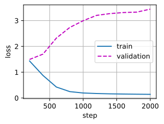
data = d2l.TimeMachine(batch_size=64, num_steps=128, tokenization='char',
                       num_train=100000, num_val=3000)

@nnx.jit
def batch_loss(model, X, Y):
    logits = model(X)
    return optax.softmax_cross_entropy_with_integer_labels(
        logits.reshape(-1, logits.shape[-1]), Y.reshape(-1)).mean()

def val_loss(model, data):
    """Mean per-token validation loss (weighted by batch size: the final
    batch may be smaller)."""
    model.eval()
    total = count = 0
    for X, Y in data.val_dataloader():
        Y = jnp.asarray(Y)
        total += float(batch_loss(model, jnp.asarray(X), Y)) * Y.size
        count += Y.size
    model.train()
    return total / count

model = GPT(len(data.vocab), dropout=0.1, rngs=nnx.Rngs(0))
optimizer = nnx.Optimizer(model, optax.adamw(1e-3, weight_decay=0.0),
                          wrt=nnx.Param)
steps, train_curve, val_curve = [], [], []
for chunk in range(10):
    losses = d2l.train_lm(model, data, optimizer, 200)
    steps.append(200 * (chunk + 1))
    train_curve.append(sum(losses[-50:]) / 50)
    val_curve.append(val_loss(model, data))
d2l.plot(steps, [train_curve, val_curve], 'step', 'loss',
         legend=['train', 'validation'])
print(f'final: train {train_curve[-1]:.2f}, '
      f'validation {val_curve[-1]:.2f}; '
      f'best validation {min(val_curve):.2f} at step '
      f'{steps[val_curve.index(min(val_curve))]}')
final: train 0.15, validation 3.19; best validation 1.46 at step 200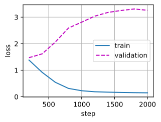
The training loss falls toward a few tenths of a nat. Validation loss reaches its minimum near \(1.5\) nats within the first few hundred steps and then rises while training loss continues to decrease. The run processes roughly 16 million tokens drawn repeatedly from about one hundred thousand characters, or about 160 passes through the corpus, with 4.7 million parameters. This train–validation divergence is consistent with memorization under repeated corpus reuse. The experiment does not isolate a remedy; larger and more varied training data is the change studied by the scaling analysis at the end of the chapter (Kaplan et al. 2020; Hoffmann et al. 2022).
The estimated training cost locates this run relative to larger models. At roughly \(6ND\) floating-point operations for training a model of \(N\) parameters on \(D\) tokens, our minute of GPU time spent about \(5 \times 10^{14}\) FLOPs. The 124M-parameter GPT-2 we load below cost on the order of \(7 \times 10^{18}\) by the same estimate, taking WebText at roughly ten billion tokens; it is the same class with about 26 times our parameter count, trained on a corpus five orders of magnitude larger. The 1.5B-parameter GPT-2 XL lands near \(10^{20}\), and frontier runs sit around \(10^{25}\) or beyond. Across those ten orders of magnitude the model definition barely changes — block, mask, embedding, head — but everything around it does: data pipelines, custom kernels, and the parallelism of Chapter 13. The block abstraction therefore transfers even though the surrounding training system changes with scale.
11.2.2.1 Effect of Normalization Placement
Section 11.1 predicted, from initialization statistics alone, that the post-LN arrangement reduces the gradients received by its attention layers’ query and key projections. We test this prediction with the same model, data, and 800-step budget at learning rate \(3 \times 10^{-3}\) — three times the rate above, still comfortable for pre-norm — with pre_norm flipped:
for pre_norm in (True, False):
    torch.manual_seed(0)
    ablation = GPT(len(data.vocab), pre_norm=pre_norm)
    losses = d2l.train_lm(ablation, data,
                          torch.optim.AdamW(ablation.parameters(), lr=3e-3,
                                            weight_decay=0.0), 800)
    print(f'pre_norm={pre_norm}: loss at step 100/200/400/800: ' +
          '/'.join(f'{sum(losses[k-50:k]) / 50:.2f}'
                   for k in (100, 200, 400, 800)))
pre_norm=True: loss at step 100/200/400/800: 2.20/1.83/1.38/1.11
pre_norm=False: loss at step 100/200/400/800: 2.83/2.83/2.83/2.83for pre_norm in (True, False):
ablation = GPT(len(data.vocab), pre_norm=pre_norm, rngs=nnx.Rngs(0))
optimizer = nnx.Optimizer(ablation, optax.adamw(3e-3, weight_decay=0.0),
wrt=nnx.Param)
losses = d2l.train_lm(ablation, data, optimizer, 800)
print(f'pre_norm={pre_norm}: loss at step 100/200/400/800: ' +
'/'.join(f'{sum(losses[k-50:k]) / 50:.2f}'
for k in (100, 200, 400, 800)))pre_norm=True: loss at step 100/200/400/800: 1.88/1.41/1.01/0.35
pre_norm=False: loss at step 100/200/400/800: 2.83/2.83/2.83/2.83The pre-norm model trains normally. The post-norm model does not diverge — no NaNs, no explosion — it does something more telling: it sticks at about \(2.8\) nats and never leaves. That number is exactly the unigram entropy of this text (\(2.83\) nats: predict letter frequencies, ignore all context), and a language model pinned there is a model whose attention has learned nothing — the training-time realization of the starved query/key gradients we measured at initialization. At the gentler learning rate of the previous run, post-LN does train, trailing early (this is what learning-rate warmup was invented for (Xiong et al. 2020)); at the rate pre-norm shrugs off, it fails outright. GPT-2 moved the normalization quietly, ahead of most of the field, and that is one reason its 48-block variant was trainable at all in 2019 (Radford et al. 2019).
11.2.3 Sampling from the Model
A language model outputs a distribution; text comes from decoding it. Section 8.7 covered the search view — greedy, beam, sampling-with-temperature — for sequence models in general. For open-ended generation the workhorse is temperature-plus-truncation: divide the logits by a temperature \(\tau\), optionally keep only the \(k\) most probable tokens (Fan et al. 2018) (or the smallest set covering probability \(p\), nucleus sampling (Holtzman et al. 2020) — an exercise), and sample. We add generate to the class. It is deliberately naive: every new token reruns the full forward pass over the whole history, which is quadratic work per token. The entire next section measures that waste and then eliminates it.
@d2l.add_to_class(GPT)
@torch.no_grad()
def generate(self, prefix, num_tokens, temperature=1.0, top_k=None):
    """Sample a continuation of the token-id list prefix."""
    ids = list(prefix)
    device = next(self.parameters()).device
    for _ in range(num_tokens):
        X = torch.tensor(ids[-self.max_len:], device=device)[None]
        logits = self(X)[0, -1] / temperature
        if top_k is not None:
            cutoff = torch.topk(logits, top_k).values[-1]
            logits[logits < cutoff] = -torch.inf
        ids.append(int(torch.multinomial(F.softmax(logits, -1), 1)))
return ids@d2l.add_to_class(GPT)
def generate(self, prefix, num_tokens, seed=0, temperature=1.0,
top_k=None):
"""Sample a continuation of the token-id list prefix."""
total = len(prefix) + num_tokens
buf = jnp.zeros((1, total), dtype=jnp.int32)
buf = buf.at[0, :len(prefix)].set(jnp.asarray(prefix))
@nnx.jit
def logits_at(model, buf, t):
return model(buf)[0, t - 1]
ids, key = list(prefix), jax.random.key(seed)
for t in range(len(prefix), total):
logits = logits_at(self, buf, t) / temperature
if top_k is not None:
logits = jnp.where(logits < jnp.sort(logits)[-top_k],
-jnp.inf, logits)
key, sub = jax.random.split(key)
ids.append(int(jax.random.categorical(sub, logits)))
buf = buf.at[0, t].set(ids[-1])
return idsOne JAX-specific choice: rather than growing the input by one token per step — which would trigger a fresh XLA compilation at every new length — we allocate a buffer of the final size once and overwrite it left to right. The causal mask makes the not-yet-written positions invisible to every query before them, so the logits at position \(t-1\) are exact, and the jitted forward compiles exactly once. Fixed shapes are how real JAX serving systems work too, as the next section shows.
Let’s hear what 4.7 million parameters trained for a minute sound like:
model.eval()
prefix = data.vocab[list('the time traveller ')]
for temperature, top_k in ((1.0, None), (0.7, 8), (2.0, None)):
    torch.manual_seed(0)
    out = model.generate(prefix, 120, temperature, top_k)
    d2l.print_wrapped(f'T={temperature}, top_k={top_k}: '
                      + repr(''.join(data.vocab.to_tokens(out))))
T=1.0, top_k=None: 'the time traveller had more than a touch of whim among
his elements and we distrusted him things that would have made the frame
of a less c'
T=0.7, top_k=8: 'the time traveller had more than a touch of whim among his
elements and we distrusted him things that would have made the frame of
a less c'
T=2.0, top_k=None: 'the time traveller had more that exceriesy of the silent
man egr and so i never talked of it until experimental verification
cried i you ar'model.eval()
prefix = data.vocab[list('the time traveller ')]
for temperature, top_k in ((1.0, None), (0.7, 8), (2.0, None)):
out = model.generate(prefix, 120, seed=0, temperature=temperature,
top_k=top_k)
d2l.print_wrapped(f'T={temperature}, top_k={top_k}: '
+ repr(''.join(data.vocab.to_tokens(out))))T=1.0, top_k=None: 'the time traveller hated to have servants waiting at
dinner for a hot plate at that the editor turned to his knife and fork
with a grunt an'
T=0.7, top_k=8: 'the time traveller stood before us i gave a cry of surprise
good heavens man what s the matter cried the medical man who saw him
next and t'
T=2.0, top_k=None: 'the time traveller hated to have seubitating across the
lower round nature azout you like to the buildings with intricate
parapets and type'The samples are fluent pseudo-Wells — and much of that fluency appears memorized rather than composed: the overfitting that the validation curve reported, made audible. Note how little the temperature changes the early tokens. A memorizing model is a confident model, and dividing near-one-hot logits by \(0.7\) or \(2\) barely moves them; the knobs only start to matter once the model is genuinely uncertain. We need a model whose uncertainty is real — so let’s load one.
11.2.4 Loading GPT-2
GPT-2 is the type specimen of this section’s class: 12 blocks, 768 hidden units, 12 heads, LayerNorm (with biases), GELU, learned positions, tied head — and pre-norm, years before that was consensus. Its 124M-parameter release is a constructor call away; all we owe it is its exact flags, plus its weights and its tokenizer, both of which we pin by content hash in d2l.DATA_HUB so that one download serves every later run and framework.
HF_URL = 'https://huggingface.co/openai-community/gpt2/resolve/main/'
d2l.DATA_HUB['gpt2-weights'] = (
    HF_URL + 'model.safetensors',
    '89a76996d7c6ee89b86618a265483aab73e61d50')
d2l.DATA_HUB['gpt2-merges'] = (
    HF_URL + 'merges.txt', '396d4d8ec90cb02f4d56e049e0e4add868bcd943')
d2l.DATA_HUB['gpt2-encoder'] = (
    HF_URL + 'vocab.json', 'f0223209235343bc067d7da838328bced8085ae1')

enc = tiktoken.Encoding(
    'gpt2', explicit_n_vocab=50257,
    pat_str=d2l.BPETokenizer.GPT2_PATTERN,
    mergeable_ranks=data_gym_to_mergeable_bpe_ranks(
        d2l.download('gpt2-merges', '../data/gpt2'),
        d2l.download('gpt2-encoder', '../data/gpt2')),
    special_tokens={'<|endoftext|>': 50256})
ids = enc.encode('Attention is all you need.')
print(ids, [enc.decode([i]) for i in ids])
[8086, 1463, 318, 477, 345, 761, 13] ['Att', 'ention', ' is', ' all', ' you', ' need', '.']HF_URL = 'https://huggingface.co/openai-community/gpt2/resolve/main/'
d2l.DATA_HUB['gpt2-weights'] = (
HF_URL + 'model.safetensors',
'89a76996d7c6ee89b86618a265483aab73e61d50')
d2l.DATA_HUB['gpt2-merges'] = (
HF_URL + 'merges.txt', '396d4d8ec90cb02f4d56e049e0e4add868bcd943')
d2l.DATA_HUB['gpt2-encoder'] = (
HF_URL + 'vocab.json', 'f0223209235343bc067d7da838328bced8085ae1')
enc = tiktoken.Encoding(
'gpt2', explicit_n_vocab=50257,
pat_str=d2l.BPETokenizer.GPT2_PATTERN,
mergeable_ranks=data_gym_to_mergeable_bpe_ranks(
d2l.download('gpt2-merges', '../data/gpt2'),
d2l.download('gpt2-encoder', '../data/gpt2')),
special_tokens={'<|endoftext|>': 50256})
ids = enc.encode('Attention is all you need.')
print(ids, [enc.decode([i]) for i in ids])[8086, 1463, 318, 477, 345, 761, 13] ['Att', 'ention', ' is', ' all', ' you', ' need', '.']The tokenizer cell applies the BPE machinery of Section 8.2 to GPT-2’s released merge list and vocabulary. It uses the same pre-tokenization pattern as d2l.BPETokenizer and assembles the result into tiktoken’s encoder. The construction requires two data files and a regular expression, without a model library or configuration framework.
The checkpoint stores one tensor per parameter under names such as h.3.attn.c_attn.weight, so loading requires a dictionary that maps these names onto our modules. One historical detail requires care: GPT-2’s original code implemented linear layers as a Conv1D class that keeps weights as \((\textrm{in}, \textrm{out})\) — the transpose of nn.Linear’s \((\textrm{out}, \textrm{in})\) — so every 2-D weight must be transposed on the way in. The fused c_attn matrix concatenates queries, keys, and values in the same order as our W_qkv, and the token embedding doubles as the output head in both models, so neither needs special handling.
gpt2 = GPT(vocab_size=50257, num_hiddens=768, num_heads=12, num_blks=12,
           max_len=1024, pos='learned', norm='layer', act='gelu',
           pre_norm=True, bias=True)  # the GPT-2 (124M) configuration
weights = load_file(d2l.download('gpt2-weights', '../data/gpt2'))

with torch.no_grad():
    gpt2.token_emb.weight.copy_(weights['wte.weight'])
    gpt2.pos_emb.weight.copy_(weights['wpe.weight'])
    gpt2.norm.weight.copy_(weights['ln_f.weight'])
    gpt2.norm.bias.copy_(weights['ln_f.bias'])
    for i, blk in enumerate(gpt2.blks):
        modules = {f'h.{i}.ln_1': blk.norm1, f'h.{i}.ln_2': blk.norm2,
                   f'h.{i}.attn.c_attn': blk.attention.W_qkv,
                   f'h.{i}.attn.c_proj': blk.attention.W_o,
                   f'h.{i}.mlp.c_fc': blk.ffn.W_1,
                   f'h.{i}.mlp.c_proj': blk.ffn.W_2}
        for key, module in modules.items():
            W = weights[key + '.weight']
            module.weight.copy_(W.T if W.ndim == 2 else W)  # Conv1D layout
            module.bias.copy_(weights[key + '.bias'])

gpt2.to(d2l.try_gpu()).eval()
print(f'{sum(p.numel() for p in gpt2.parameters()) / 1e6:.1f}M parameters')
124.4M parametersgpt2 = GPT(vocab_size=50257, num_hiddens=768, num_heads=12, num_blks=12,
max_len=1024, pos='learned', norm='layer', act='gelu',
pre_norm=True, bias=True) # the GPT-2 (124M) configuration
weights = safetensors_numpy.load_file(
d2l.download('gpt2-weights', '../data/gpt2'))
gpt2.token_emb.embedding[...] = jnp.asarray(weights['wte.weight'])
gpt2.pos_emb.embedding[...] = jnp.asarray(weights['wpe.weight'])
gpt2.norm.scale[...] = jnp.asarray(weights['ln_f.weight'])
gpt2.norm.bias[...] = jnp.asarray(weights['ln_f.bias'])
for i, blk in enumerate(gpt2.blks):
for norm, key in ((blk.norm1, f'h.{i}.ln_1'),
(blk.norm2, f'h.{i}.ln_2')):
norm.scale[...] = jnp.asarray(weights[key + '.weight'])
norm.bias[...] = jnp.asarray(weights[key + '.bias'])
for linear, key in ((blk.attention.W_qkv, f'h.{i}.attn.c_attn'),
(blk.attention.W_o, f'h.{i}.attn.c_proj'),
(blk.ffn.W_1, f'h.{i}.mlp.c_fc'),
(blk.ffn.W_2, f'h.{i}.mlp.c_proj')):
# Conv1D stores (in, out) -- exactly nnx.Linear's kernel layout
linear.kernel[...] = jnp.asarray(weights[key + '.weight'])
linear.bias[...] = jnp.asarray(weights[key + '.bias'])
gpt2.eval()
n = sum(p.size for p in jax.tree.leaves(nnx.state(gpt2, nnx.Param)))
print(f'{n / 1e6:.1f}M parameters')124.4M parametersLoading takes no torch and no transposes here: the safetensors file opens directly into NumPy arrays, and the Conv1D \((\textrm{in}, \textrm{out})\) layout that PyTorch users must transpose happens to be exactly the layout nnx.Linear keeps its kernels in.
Shape checks alone do not validate a loaded checkpoint because a transposed square matrix still multiplies. We therefore use a quantitative loss check and a generated-text check. First, the model should assign natural English a plausible probability:
text = ("The Time Machine, by H. G. Wells. The Time Traveller was "
        "expounding a recondite matter to us.")
x = torch.tensor(enc.encode(text), device=d2l.try_gpu())[None]
with torch.no_grad():
    logits = gpt2(x)
loss = F.cross_entropy(logits[0, :-1], x[0, 1:])
print(f'per-token loss {loss.item():.2f}, '
      f'perplexity {loss.exp().item():.0f}')
per-token loss 3.89, perplexity 49text = ("The Time Machine, by H. G. Wells. The Time Traveller was "
"expounding a recondite matter to us.")
x = jnp.asarray(enc.encode(text))[None]
loss = optax.softmax_cross_entropy_with_integer_labels(
gpt2(x)[0, :-1], x[0, 1:]).mean()
print(f'per-token loss {loss:.2f}, perplexity {jnp.exp(loss):.0f}')per-token loss 3.89, perplexity 49A per-token perplexity around 50 says the plumbing is right: the vocabulary is 50,257-way, and uniform guessing would score 50,257. Second, the readable check: greedy decoding of a stock prompt reproduces GPT-2’s well-documented continuation, and sampled continuations respond to the temperature and top-\(k\) knobs the way the char model could not:
torch.manual_seed(0)
out = gpt2.generate(enc.encode('Alan Turing theorized that computers '
                               'would one day become'), 16, top_k=1)
d2l.print_wrapped(enc.decode(out))
torch.manual_seed(0)
out = gpt2.generate(enc.encode('The secret of a good deep learning '
                               'textbook is'), 40, temperature=0.8,
                    top_k=50)
d2l.print_wrapped(enc.decode(out))
Alan Turing theorized that computers would one day become the most powerful
machines on the planet.
The computer is a machine that
The secret of a good deep learning textbook is that you don't know what
you're supposed to write. That's not quite right, but it's a good idea.
So let's dive into the book for a second.out = gpt2.generate(enc.encode('Alan Turing theorized that computers '
'would one day become'), 16, top_k=1)
d2l.print_wrapped(enc.decode(out))
out = gpt2.generate(enc.encode('The secret of a good deep learning '
'textbook is'), 40, seed=0, temperature=0.8,
top_k=50)
d2l.print_wrapped(enc.decode(out))Alan Turing theorized that computers would one day become the most powerful
machines on the planet.
The computer is a computer that
The secret of a good deep learning textbook is to make sure that you have
the right skills set to get started.
A good deep learning textbook is to make sure you have the right skills set
to get started.
I used toWith five configuration choices, the class developed here can load and run GPT-2. The difference between our short training run and GPT-2 lies primarily in the amounts of data and computation, together with the engineering needed to use them. The following sections examine efficient generation with a KV cache, encoder and encoder–decoder variants, mixture-of-experts layers, and the relation between scale and performance. The configurations of Llama, Qwen, and DeepSeek will then be expressed in terms of the same class.
11.2.5 Summary
A GPT consists of a token embedding, causally masked transformer blocks, a final normalization layer, and an output head tied to the embedding. Positions can be represented by a learned table, as in GPT-2, or by RoPE inside each attention head. Our GPT class exposes these choices and inserts causal attention through the attn_factory interface of d2l.TransformerBlock. On the 180 KB training text, validation loss reaches its minimum within a few hundred steps and then rises as the model memorizes the corpus. With post-norm at the same learning rate, training remains near the unigram entropy, consistent with the gradient attenuation measured in the preceding section. Temperature and truncation control sampling. The released 124M-parameter GPT-2 checkpoint loads into the same class through a parameter-name mapping, with the Conv1D matrices transposed in PyTorch and left unchanged in JAX. The loaded model passes a perplexity check and produces coherent completions for the example prompts.
11.2.6 Exercises
Parameter census. The loading code of Section 11.2.4 reports 124.4M parameters for the GPT-2 configuration, which has width \(d = 768\), 12 blocks, a vocabulary of \(V = 50{,}257\) tokens, and 1,024 positions.
- Count the parameters of one block exactly, including the biases of its four linear layers and the gains and shifts of its two LayerNorms. Add the token table, the position table, and the final normalization, and verify that the total is \(124{,}439{,}808\).
- Exercise 8 of Section 11.1 gives the exact parameter count of the default
TransformerBlock, whichGPTbuilds with its default flags. Use it to count the parameters ofGPT(vocab_size=28), with \(d = 256\) and six blocks, and check the total against the count printed in Section 11.2.1. What fraction of the parameters sits in the embedding tables of each of the two models? - Without tying, the output head would be a separate \(V \times d\) matrix. How many parameters would GPT-2 then have? A product of a \(d_\textrm{out} \times d_\textrm{in}\) matrix with a vector costs about \(2 d_\textrm{out} d_\textrm{in}\) floating-point operations, and a table lookup costs none. Estimate the share of GPT-2’s per-token matrix work that the head accounts for at short contexts, where the attention scores are negligible, and compare it with the share of the parameters that the shared table holds.
[code] Unmasked attention. In
GPT, the flagis_causal=Trueof the attention call inCausalAttentionis the only mechanism that keeps position \(t\) from attending to later positions.- Take one validation sequence of 128 characters and replace its character at position 64 by a different one. For every position, compute the largest absolute change of the logits of the trained
model, and plot the change against position. - Subclass
GPTwith a nestedCausalAttentionwhose attention call passesis_causal=False. Train it with the settings of Section 11.2.2 for 200 steps. Compare its training and validation losses with those that the training ofmodelrecords at step 200, and explain the numbers. - Sample 100 characters from the unmasked model with the prefix
'the time traveller '. Explain why the validation loss of the previous sub-problem and this sample judge the unmasked model so differently.
- Take one validation sequence of 128 characters and replace its character at position 64 by a different one. For every position, compute the largest absolute change of the logits of the trained
[code] Loss baselines. Simple predictors give reference levels for the losses of Section 11.2.2. Let the training text be the first 100,128 characters of the preprocessed corpus
data._preprocess(data._download()), which are the characters that the training windows cover. Compute three cross-entropies on the training text in nats per character: that of the uniform distribution over the 28 vocabulary entries, that of the unigram distribution of the training text, and that of the bigram model, which predicts each character from the previous one with the conditional frequencies of the training text. Check the unigram value against the 2.83 nats quoted in[code] Tied head without blocks. ● Consider
GPTwithnum_blks=0and its defaultspos='rope'andnorm='rms'. Let \(\mathbf{e}_1, \ldots, \mathbf{e}_V \in \mathbb{R}^d\) be the rows of the token table, let \(\boldsymbol{\gamma}\) be the gain of the final RMSNorm Equation 11.1.3, and let \(z_{ij}\) be the logit of token \(j\) when the current token is \(i\).Show that \(z_{ij} = s_i M_{ij}\) with scalars \(s_i > 0\) and a symmetric matrix \(\mathbf{M}\), and express \(s_i\) and \(\mathbf{M}\) in terms of the table and \(\boldsymbol{\gamma}\).
For three distinct tokens \(i\), \(j\), and \(k\), show that
\[\frac{z_{ij} - z_{ik}}{s_i} + \frac{z_{jk} - z_{ji}}{s_j} + \frac{z_{ki} - z_{kj}}{s_k} = 0. \tag{11.2.1}\]
Conclude that on the periodic text \(ijk\,ijk\,ijk \ldots\) the model assigns the correct next token a probability of at most \(1/2\) in at least one of the three contexts, so that its average loss exceeds \((\ln 2)/3\) nats per token. Which loss can a model with an untied head reach on this text?
Show that losses arbitrarily close to \((\ln 2)/3\) are attainable.
Train
GPT(len(data.vocab), num_blks=0)for 2,000 steps with the optimizer of Section 11.2.2 at learning rate \(10^{-2}\), and compare its final training loss with the bigram cross-entropy of problem 3. Use the first sub-problem to explain the difference.
[code] Verbatim recall. Section 11.2.3 attributes much of the fluency of the samples of
modelto memorization. A sample that copies its training text contains long strings that occur in that text verbatim. Let the training text be as in problem 3.- Draw ten samples of 100 characters from
modelat temperature 1 without truncation, with the prefix'the time traveller 'and ten different seeds. Compute the verbatim fraction of each sample, the fraction of its 20-character windows that occur verbatim in the training text. As a reference, compute the same fraction for the 2,000 characters of the preprocessed corpus from position 103,128 on, which lie beyond both the training and the validation windows. - Retrain the model with the settings of Section 11.2.2, stop at the step at which the validation loss was lowest, and repeat the measurement.
- Retrain with
dropout=0.3for the full 2,000 steps. Compare its lowest validation loss, the step at which that loss occurs, and its verbatim fraction at the end of training with those of the two previous models.
- Draw ten samples of 100 characters from
[code] Post-norm plateau. ● Section 11.2.2.1 reads the post-norm loss of about 2.8 nats as the loss of a model whose attention has learned nothing.
- Suppose that every attention sublayer of the post-norm model outputs zero, while its FFN sublayers still act on every position. Which of the losses of problem 3 can such a model still reach? What does a plateau at the unigram entropy imply about how the predictions depend on the current character?
- Train the post-norm ablation for 800 steps at learning rate \(3 \times 10^{-3}\). On a validation batch, measure the mean KL divergence of its predictive distributions from the unigram distribution of the training text. Then apply
token_emband the blocks ofblksone at a time, and record after each block the token spread \(\|\mathbf{H} - \bar{\mathbf{H}}\| / \|\mathbf{H}\|\) of Section 11.1.2.2, averaged over the sequences of the batch, both for the trained model and for a freshly initialized post-norm model. After which block, if any, have the tokens of the trained model collapsed, and how did training change the profile of the initialized model? - Add a linear warmup of the learning rate from 0 to \(3 \times 10^{-3}\) over the first 200 steps and repeat the 800-step run. Does the post-norm model leave the plateau, and how does its loss at step 800 compare with that of the pre-norm run of Section 11.2.2.1?
[code] Temperature limits.
generatedivides the logits \(\mathbf{z}\) by the temperature \(\tau\) before the softmax.- Show that as \(\tau \to 0\) the sampling distribution converges to the one-hot vector on the largest logit, assuming that this logit is unique, and that as \(\tau \to \infty\) it converges to the uniform distribution over the vocabulary.
- For the trained
model, sample 100 characters with the prefix'the time traveller 'at each \(\tau \in \{0.5, 1, 2, 4\}\) without truncation. At every generated position, compute the entropy of the tempered distribution \(\mathrm{softmax}(\mathbf{z}/\tau)\), and average over positions. Plot the averages against \(\tau\) together with the limits \(0\) and \(\ln 28\), and relate the result to the observation of Section 11.2.3 that the temperature changes the early tokens of the samples little.
[code] Nucleus sampling. Nucleus or top-\(p\) sampling (Holtzman et al. 2020) keeps the smallest set of most probable tokens whose probabilities sum to at least \(p\), renormalizes the probabilities over this set, and samples from it.
sample_nextof Section 8.7 implements it, and that section argues that it adapts to the confidence of the model while top-\(k\) does not.- Add an argument
top_ptogeneratethat applies this rule after the temperature. Check thattop_p=1leaves the sampling distribution unchanged and that a very smalltop_preproduces greedy decoding. - With
gpt2, generate 40 tokens withtop_k=50and, under the same seed, withtop_p=0.9. Do so once for a prompt whose continuation is nearly determined, such as the opening words of a well-known quotation, and once for an open-ended prompt. At every step, record the entropy of the model’s distribution, the number of tokens that the nucleus keeps, and the probability mass that top-\(k\) discards. Plot the last two quantities against the entropy. Below which entropy does the nucleus keep fewer than 5 of the 50 tokens that top-\(k\) admits, and above which entropy does top-\(k\) discard more than a tenth of the mass?
Adapted from Stanford CS336, Assignment 1, Problem (decoding).
- Add an argument
[code] Checkpoint mismatches. The GPT-2 checkpoint holds 160 tensors with 137,022,720 numbers in all, while
gpt2has 124,439,808 parameters.- Identify the checkpoint tensors that the loading code of Section 11.2.4 never reads, and explain why
GPTneeds no counterpart for them. - Construct the GPT-2 configuration with
norm='rms'and run the loading code. Which line fails, and why can no mapping of the checkpoint onto this configuration reproduce GPT-2? Then list, for the GPT-2 configuration withpos='rope'andact='swiglu', every checkpoint tensor without a destination and every model parameter without a source. - Some mistakes load without any error. Introduce three of them, one at a time: skip every copy of a normalization shift and load the rest into the
norm='rms'model; load theattn.c_projmatrix of every block in the wrong orientation, which no shape check detects because the matrix is square; and swap the query and key thirds of everyc_attnweight and bias. For each mistake, report the perplexity of the sentence that Section 11.2.4 scores and the greedy continuation of the prompt'Alan Turing theorized that computers would one day become'. Which mistake does the perplexity check flag most clearly, and which least?
- Identify the checkpoint tensors that the loading code of Section 11.2.4 never reads, and explain why
[code] Learned position table. The rows \(\mathbf{p}_0, \ldots, \mathbf{p}_{1023}\) of
gpt2.pos_embwere learned freely, without the structure of the sinusoidal table Equation 10.4.2.- Compute the norm of every row and plot it against position. Which rows stand out? What distinguishes position 0 from every other position in a causal model?
- Exercise 4 of Section 10.4 tested the trained table of
TinyCharLMfor shift invariance by comparing the spread of the cosine similarities along each diagonal \(i - j = \textrm{const}\) with the spread of the diagonal means. Display the cosine similarities between all rows ofgpt2.pos_embwithd2l.show_heatmaps, apply the same test, and compare the outcome with that of the 128 rows trained at context 128 there. - Center the table and compute its singular value decomposition. What fraction of the variance do the top three singular directions capture? Plot the projections of the rows onto these directions against position, and describe the curve that the rows trace in this three-dimensional subspace. Which features of a sinusoidal table does it share?
[code] Bits per character. ● GPT-2 and
modeluse different tokens, so their per-token losses are not comparable. A loss of \(\ell\) nats per token at \(c\) characters per token corresponds to\[\frac{\ell}{c \ln 2} \textrm{ bits per character}. \tag{11.2.2}\]
Take as held-out passage the last 20,000 characters of the raw text
data._download(). After preprocessing, they lie beyond the validation windows.- Compute the bits per character of
modelon the preprocessed passage, in non-overlapping windows of 128 characters. - Compute the bits per character of
gpt2on the same preprocessed passage in chunks of 1,024 tokens. Repeat on the raw passage, with its capitalization, punctuation, and line breaks. - Which of the two GPT-2 figures should be compared with that of
model? Discuss what each side brings to the passage:modelwas trained on the same novel, sees 128 characters of context, and predicts 28 symbols, whereas GPT-2 was trained on 40 GB of WebText, sees up to 1,024 tokens, and predicts 50,257 symbols.
- Compute the bits per character of
[extended] Subwords at small scale. ● Section 11.2.1 trains on characters because, on a 180 KB novel, a subword vocabulary would leave each token type a handful of training examples.
d2l.TimeMachinewithtokenization='bpe'and a givenvocab_sizetrains aBPETokenizeron the text and tokenizes with it. Test the argument.- Subclass
d2l.TimeMachineso that_downloadreturns the preprocessed text, which gives both tokenizations the same characters. Choosenum_trainandnum_valso that the training and validation windows cover the same characters as those of Section 11.2.2. Withvocab_size=256the tokenizer learns no merges; check thatGPTthen reaches validation losses close to those ofmodelat the same steps. - For each of the vocabulary sizes 512, 1,024, and 2,048, choose
num_trainandnum_valas in the previous sub-problem, and trainGPTwith the other settings of Section 11.2.2. Convert the lowest validation loss of each run to bits per character as in problem 11. Record also how often the median token type of each vocabulary occurs in the tokenized training text, counting only the types that occur at least once. - With
num_steps=128, a larger vocabulary also gives the model more characters of context. Repeat the best vocabulary size with anum_stepsat which a window covers about 128 characters, and decide whether the argument of Section 11.2.1 holds at this corpus size.
- Subclass