import time
import torch
from torch import nn
from torch.nn import functional as F
from torch.utils.checkpoint import checkpoint
from d2l import torch as d2l5.7 GPUs, Devices, and Memory
Training beyond small examples usually runs on an accelerator, most often a CUDA GPU. This introduces two practical constraints. Every tensor and parameter has a device, and an operation generally requires its inputs to be on the same device. GPU memory is also much smaller than main memory and often limits the model or batch size. The section is organized around three operational questions: where arrays and state live; what occupies training memory and how checkpointing changes it; and when asynchronous execution or data transfer forces synchronization. The examples fall back to the CPU when no GPU is available, but CPU execution verifies API shape rather than GPU performance.
import os
os.environ['TF_CPP_MIN_LOG_LEVEL'] = '2'
import time
import numpy as np
import tensorflow as tf
from d2l import tensorflow as d2l
import time
import jax
from jax import numpy as jnp
from flax import nnx
import optax
from d2l import jax as d2limport time
from d2l import mxnet as d2l
from mxnet import np, npx
from mxnet.gluon import nn
npx.set_np()5.7.1 Devices and Placement
In PyTorch every tensor carries a device. The CPU is torch.device('cpu') and it stands for all physical CPU cores and all of main memory. A CUDA device such as torch.device('cuda:0') is one specific card and its own memory; on a machine with several GPUs, cuda:1 is the second card, and plain 'cuda' is shorthand for cuda:0. To see what your machine has, run nvidia-smi in a shell: it lists every card, its memory, and what is currently running on it. We wrap device construction in two helpers that the rest of the book uses.
TensorFlow names devices with strings. '/CPU:0' is the CPU and it stands for all physical CPU cores and all of main memory; '/GPU:0' is one specific CUDA card and its own memory, and '/GPU:1' is the second card. tf.device turns a name into a scope: operations executed inside it run on, and allocate their results on, the named device. To see what your machine has, run nvidia-smi in a shell: it lists every card, its memory, and what is currently running on it. We wrap device construction in two helpers that the rest of the book uses.
In JAX every array lives on a device, and jax.devices(backend) returns the device handles of a backend. jax.devices('cpu')[0] is the CPU, and it stands for all physical CPU cores and all of main memory; jax.devices('gpu')[i] is one specific CUDA card and its own memory. To see what your machine has, run nvidia-smi in a shell: it lists every card, its memory, and what is currently running on it. We wrap device lookup in two helpers that the rest of the book uses.
In MXNet every array carries a device. The CPU is npx.cpu() and it stands for all physical CPU cores and all of main memory; npx.gpu(i) is one specific CUDA card and its own memory, and npx.gpu() is shorthand for npx.gpu(0). MXNet 1.x called this object a context, and most MXNet code you will find online writes ctx=; MXNet 2.0 renamed it to device (Context survives only as a deprecated alias of Device), and every ctx spelling in this book’s MXNet code is accepted as a compatibility form of device. To see what your machine has, run nvidia-smi in a shell: it lists every card, its memory, and what is currently running on it. We wrap device construction in two helpers that the rest of the book uses.
def cpu():
    """Get the CPU device."""
    return torch.device('cpu')

def gpu(i=0):
    """Get a GPU device."""
    return torch.device(f'cuda:{i}')

cpu(), gpu(), gpu(1)
(device(type='cpu'),
device(type='cuda', index=0),
device(type='cuda', index=1))def cpu():
"""Get the CPU device."""
return tf.device('/CPU:0')
def gpu(i=0):
"""Get a GPU device."""
return tf.device(f'/GPU:{i}')
cpu(), gpu(), gpu(1)(<tensorflow.python.eager.context._EagerDeviceContext at 0x758883906c00>,
<tensorflow.python.eager.context._EagerDeviceContext at 0x758883c9c6c0>,
<tensorflow.python.eager.context._EagerDeviceContext at 0x75887c23df80>)def cpu():
"""Get the CPU device."""
return jax.devices('cpu')[0]
def gpu(i=0):
"""Get a GPU device."""
return jax.devices('gpu')[i]
cpu()CpuDevice(id=0)def cpu():
"""Get the CPU device."""
return npx.cpu()
def gpu(i=0):
"""Get a GPU device."""
return npx.gpu(i)
cpu(), gpu(), gpu(1)(cpu(0), gpu(0), gpu(1))Note that constructing a device object is free and always succeeds, whether or not the hardware exists; the check happens only when you try to put data on it.
Note that constructing a device scope is free and always succeeds, whether or not the hardware exists; the name is checked only when an operation runs inside the scope. Even then, TensorFlow’s default soft placement falls back to the CPU rather than raising when the requested device is missing, which is what lets gpu(1) print happily on a laptop. Soft placement can therefore mask an unavailable requested device; inspect x.device when placement matters.
Note that a JAX device object is a handle to hardware that actually exists: jax.devices('gpu') raises a RuntimeError when no GPU backend is present, rather than returning a placeholder (which is why the demo above calls only cpu()). Our next helper therefore counts GPUs through a try/except.
Note that constructing a Device is free and always succeeds, whether or not the hardware exists; the check happens only when you try to put data on it.
We can query how many GPUs are actually available.
def num_gpus():
    """Get the number of available GPUs."""
    return torch.cuda.device_count()

num_gpus()2def num_gpus():
"""Get the number of available GPUs."""
return len(tf.config.experimental.list_physical_devices('GPU'))
num_gpus()2def num_gpus():
"""Get the number of available GPUs."""
try:
return jax.device_count('gpu')
except:
return 0 # No GPU backend found
num_gpus()2def num_gpus():
"""Get the number of available GPUs."""
return npx.num_gpus()
num_gpus()2Now we define two convenient functions that allow us to run code even if the requested GPUs do not exist.
def try_gpu(i=0):
    """Return gpu(i) if exists, otherwise return cpu()."""
    if num_gpus() >= i + 1:
        return gpu(i)
    return cpu()

def try_all_gpus():
    """Return all available GPUs, or [cpu(),] if no GPU exists."""
    devices = [gpu(i) for i in range(num_gpus())]
    return devices if devices else [cpu()]

try_gpu(), try_gpu(10), try_all_gpus()(device(type='cuda', index=0),
device(type='cpu'),
[device(type='cuda', index=0), device(type='cuda', index=1)])(<tensorflow.python.eager.context._EagerDeviceContext at 0x75887c245880>,
<tensorflow.python.eager.context._EagerDeviceContext at 0x75887c245600>,
[<tensorflow.python.eager.context._EagerDeviceContext at 0x75887c2455c0>,
<tensorflow.python.eager.context._EagerDeviceContext at 0x75887c245580>])(CudaDevice(id=0), CpuDevice(id=0), [CudaDevice(id=0), CudaDevice(id=1)])(gpu(0), cpu(0), [gpu(0), gpu(1)])CUDA is not the only accelerator string PyTorch understands. Apple-silicon Macs expose their GPU as mps, Intel GPUs appear as xpu, and TPUs are reachable through JAX; PyTorch now bundles the whole family behind the torch.accelerator namespace, whose device_count() and current_accelerator() do generically what our helpers do for CUDA. We keep our own helpers anyway: they give all four of the book’s implementations one vocabulary, and they degrade to the CPU instead of failing, which is exactly what lets this book’s code run unchanged on a laptop. The book standardizes on CPU plus CUDA. Most placement and accounting concepts below also apply to other accelerators, although their APIs and supported operations differ.
CUDA is not the only accelerator TensorFlow understands: the same device strings name TPUs ('/TPU:0') on a TPU host, and the tensorflow-metal plugin exposes an Apple-silicon GPU as '/GPU:0'; tf.config.list_physical_devices() with no argument lists everything the runtime can see. We keep our own helpers anyway: they give all four of the book’s implementations one vocabulary, and they degrade to the CPU instead of failing, which is exactly what lets this book’s code run unchanged on a laptop. The book standardizes on CPU plus CUDA. Most placement and accounting concepts below also apply to other backends, although their APIs and supported operations differ.
CUDA is not the only backend JAX understands: the same program runs on CPU, GPU, or TPU, and plain jax.devices() lists the devices of the default backend, which is the best accelerator present. We keep our own helpers anyway: they give all four of the book’s implementations one vocabulary, and they degrade to the CPU instead of failing, which is exactly what lets this book’s code run unchanged on a laptop. The book standardizes on CPU plus CUDA. Most placement and accounting concepts below also apply to TPUs, although backend behavior can differ.
MXNet’s device zoo is the smallest of the four: CPU and CUDA GPUs, plus one special citizen, npx.cpu_pinned(), which names page-locked host memory and returns later in this section when we discuss transfers. MXNet’s development is archived, so no wider family is coming. We keep our own helpers anyway: they give all four of the book’s implementations one vocabulary, and they degrade to the CPU instead of failing, which is exactly what lets this book’s code run unchanged on a laptop.
5.7.1.1 Tensors, Models, and Devices
By default, tensors are created on the CPU. We can query where a tensor lives.
By default, tensors are created on the first GPU whenever one exists and on the CPU otherwise: eager TensorFlow places every new tensor on '/GPU:0' if it can. We can query where a tensor lives.
By default, arrays are created on the default device, the first accelerator when one exists and the CPU otherwise. We can query where an array lives.
By default, tensors are created on the CPU. We can query where a tensor lives; .ctx is the historical spelling of the .device property, and both work in MXNet 2.0.
x = torch.tensor([1, 2, 3])
x.devicedevice(type='cpu')x = tf.constant([1.0, 2.0, 3.0])
x.device'/job:localhost/replica:0/task:0/device:GPU:0'x = jnp.array([1, 2, 3])
x.deviceCudaDevice(id=0)x = np.array([1, 2, 3])
x.ctxcpu(0)To create a tensor somewhere else, pass a device argument. Creating data directly on the target device is better than creating it on the CPU and moving it: the tensor then never occupies main memory or crosses the bus at all.
To place a tensor somewhere specific, create it inside a device scope: everything executed under with try_gpu(): allocates its results on that device. Creating data directly on the target device is better than creating it on the CPU and moving it: the tensor then never occupies main memory or crosses the bus at all.
To place an array somewhere specific, jax.device_put(x, device) copies it there, and the result is committed to that device: JAX will keep it and every computation on it exactly where you said. Arrays created without an explicit placement, like x above, are uncommitted; they sit on the default device but JAX may treat them as movable when they meet committed data.
To create a tensor somewhere else, pass a ctx argument (2.0 also accepts the newer spelling device). Creating data directly on the target device is better than creating it on the CPU and moving it: the tensor then never occupies main memory or crosses the bus at all.
X = torch.ones(2, 3, device=try_gpu())
X
tensor([[1., 1., 1.],
[1., 1., 1.]], device='cuda:0')with try_gpu():
X = tf.ones((2, 3))
X<tf.Tensor: shape=(2, 3), dtype=float32, numpy=
array([[1., 1., 1.],
[1., 1., 1.]], dtype=float32)>X = jax.device_put(jnp.ones((2, 3)), try_gpu())
XArray([[1., 1., 1.],
[1., 1., 1.]], dtype=float32)X = np.ones((2, 3), ctx=try_gpu())
Xarray([[1., 1., 1.],
[1., 1., 1.]], device=gpu(0))On a machine with two GPUs we can put a second tensor on the second card (on your machine, try_gpu(1) substitutes whatever is available).
Y = torch.rand(2, 3, device=try_gpu(1))
Y
tensor([[0.0769, 0.4852, 0.9990],
[0.3158, 0.7800, 0.9361]], device='cuda:1')with try_gpu(1):
Y = tf.random.uniform((2, 3))
Y<tf.Tensor: shape=(2, 3), dtype=float32, numpy=
array([[0.420228 , 0.25577712, 0.6758996 ],
[0.85069597, 0.7197846 , 0.03151751]], dtype=float32)>Y = jax.device_put(jax.random.uniform(jax.random.key(0), (2, 3)),
try_gpu(1))
YArray([[0.947667 , 0.9785799 , 0.33229148],
[0.46866846, 0.5698887 , 0.16550303]], dtype=float32)Y = np.random.uniform(size=(2, 3), ctx=try_gpu(1))
Yarray([[0.13094102, 0.38239557, 0.9510336 ],
[0.31433177, 0.23414226, 0.12296525]], device=gpu(1))5.7.1.2 Copying Between Devices
Whenever we operate on multiple tensors, they need to be on the same device. If X sits on the first GPU and Y on the second, X + Y raises RuntimeError: Expected all tensors to be on the same device. PyTorch does not choose an implicit transfer because it would make the communication cost invisible at the call site. We instead copy explicitly, as in Figure 5.7.1, and then add.
Whenever we operate on multiple tensors, they should be on the same device. TensorFlow’s eager device policy defaults to silent, so if X sits on the first GPU and Y on the second, X + Y does not raise. TensorFlow copies one operand across and returns a result. This implicit transfer incurs communication cost that is not visible at the call site. tf.config.experimental.set_device_policy('explicit') opts into strictness, turning silent copies into errors. Either way the discipline is the same: copy explicitly, as in Figure 5.7.1, and then add. The explicit copy in TensorFlow is tf.identity inside a device scope.
Whenever we operate on multiple arrays, they need to be on the same device. Uncommitted arrays are flexible: JAX decides where the result lives. But X is committed to the first GPU and Y to the second, and adding them raises an error about arrays on different devices. JAX does not choose between two explicit placements because an implicit transfer would make the communication cost invisible at the call site. We instead copy explicitly, as in Figure 5.7.1, and then add.
Whenever we operate on multiple tensors, they need to be on the same device. If X sits on the first GPU and Y on the second, X + Y raises an error: the execution engine cannot find its operands on one device and refuses to guess where the result should live. An implicit transfer would make the communication cost invisible at the call site. We instead copy explicitly, as in Figure 5.7.1, and then add.
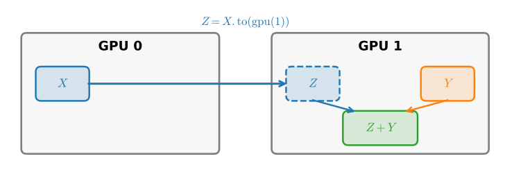
Z = X.to(try_gpu(1))
print(X)
print(Z)
tensor([[1., 1., 1.],
[1., 1., 1.]], device='cuda:0')
tensor([[1., 1., 1.],
[1., 1., 1.]], device='cuda:1')with try_gpu(1):
Z = tf.identity(X)
print(X)
print(Z)tf.Tensor(
[[1. 1. 1.]
[1. 1. 1.]], shape=(2, 3), dtype=float32)
tf.Tensor(
[[1. 1. 1.]
[1. 1. 1.]], shape=(2, 3), dtype=float32)Z = jax.device_put(X, try_gpu(1))
print(X)
print(Z)[[1. 1. 1.]
[1. 1. 1.]]
[[1. 1. 1.]
[1. 1. 1.]]Z = X.copyto(try_gpu(1))
print(X)
print(Z)[[1. 1. 1.]
[1. 1. 1.]] @gpu(0)
[[1. 1. 1.]
[1. 1. 1.]] @gpu(1)Now that Z and Y live on the same device, we can add them.
Y + Ztensor([[1.0769, 1.4852, 1.9990],
[1.3158, 1.7800, 1.9361]], device='cuda:1')Y + Z<tf.Tensor: shape=(2, 3), dtype=float32, numpy=
array([[1.420228 , 1.2557771, 1.6758996],
[1.850696 , 1.7197846, 1.0315175]], dtype=float32)>Y + ZArray([[1.947667 , 1.9785799, 1.3322915],
[1.4686685, 1.5698887, 1.165503 ]], dtype=float32)Y + Zarray([[1.130941 , 1.3823955, 1.9510336],
[1.3143318, 1.2341423, 1.1229652]], device=gpu(1))What if Z already lives on the target device? Then .to returns Z itself rather than making a copy, so calling it defensively costs nothing.
What if Z already lives on the target device? tf.identity under a scope naming that same device stays put: no bus transfer happens, so the defensive copy costs a kernel launch and nothing more. In everyday TensorFlow you will rarely write even that much, since the silent policy fetches remote operands on demand; the point of spelling out the copy is to make the one expensive transfer visible in your code instead of buried in an operator.
What if Z already lives on the target device? Then device_put skips the transfer: the array it returns shares Z’s buffer, so calling it defensively costs nothing. Comparing the buffer addresses confirms that no copy was made.
What if Z already lives on the target device? copyto would still copy, allocating fresh memory on the same device. The defensive method is as_in_ctx (whose 2.0 name is to_device): if the array already lives on the requested device it returns the array itself, so calling it defensively costs nothing. Unless you specifically want a second copy, as_in_ctx is the method of choice.
Z.to(try_gpu(1)) is ZTrueZ2 = jax.device_put(Z, try_gpu(1))
Z2.unsafe_buffer_pointer() == Z.unsafe_buffer_pointer()TrueZ.as_in_ctx(try_gpu(1)) is ZTrueThe reason for keeping copies explicit is the cost model. Accelerators can have much higher arithmetic throughput than host-to-device bandwidth, so a transfer inside a frequently executed computation can dominate its runtime. Move data to the device at the computation boundary and keep operations in the training loop on one device. Batching transfers also reduces per-transfer overhead.
5.7.1.3 Models on a Device
A model is a tree of parameter tensors, and net.to(device) moves the whole tree in one call.
A Keras model has no device argument and no move method: layers create their variables on the first call, and the variables live wherever that first call ran. So we run the first forward pass inside a device scope, and the parameters stay on that device from then on.
An NNX model owns a state tree, and jax.device_put accepts that tree. Update the model with the placed state and every registered leaf moves together.
A Gluon model does not allocate its parameters at construction: initialize(ctx=...) records the target device, and the first forward pass, which reveals the input shapes, creates every parameter there. One call therefore places the whole model.
net = nn.Sequential(nn.LazyLinear(1))
net = net.to(device=try_gpu())
net(X)
tensor([[0.5078],
[0.5078]], device='cuda:0', grad_fn=<AddmmBackward0>)net = tf.keras.Sequential([tf.keras.layers.Dense(1)])
with try_gpu():
Y_hat = net(X) # The first call creates the variables inside the scope
Y_hat<tf.Tensor: shape=(2, 1), dtype=float32, numpy=
array([[-0.9162799],
[-0.9162799]], dtype=float32)>net = nnx.Sequential(nnx.Linear(X.shape[-1], 1, rngs=nnx.Rngs(0)))
nnx.update(net, jax.device_put(nnx.state(net), try_gpu()))
net(X)Array([[-0.4064557],
[-0.4064557]], dtype=float32)net = nn.Sequential()
net.add(nn.Dense(1))
net.initialize(ctx=try_gpu())
net(X)array([[0.04115244],
[0.04115244]], device=gpu(0))The input and parameters reside on the device, so the output is computed and stored there as well. The next cell reports the parameter locations.
net[0].weight.devicedevice(type='cuda', index=0)net.layers[0].kernel.value.device'/job:localhost/replica:0/task:0/device:GPU:0'jax.tree_util.tree_map(lambda p: p.device, nnx.state(net))State({
'layers': {
0: {
'bias': Param(
value=CudaDevice(id=0)
),
'kernel': Param(
value=CudaDevice(id=0)
)
}
}
})net[0].weight.data().ctxgpu(0)Two rules keep models device-clean. Move the model before constructing the optimizer, so that the optimizer’s state is created alongside the parameters it updates. And when forward needs a fresh tensor, create it on the input’s device (torch.zeros(n, device=X.device)) rather than on the default CPU; non-parameter state that should follow the model belongs in a buffer (Section 5.2), which .to(device) moves along with everything else.
Device hygiene is short in TensorFlow because placement follows execution. A fresh tensor made during the forward pass is created where the surrounding ops run, and a Keras optimizer creates its slot variables at the first apply_gradients, next to the variables they update, so ordering takes care of itself. The one rule to remember is the first-call rule above: run the variable-building forward pass under the device scope you mean, because moving the variables afterwards means rebuilding the model.
Device hygiene is short in JAX because all state is explicit. The optimizer’s state is built from the model’s parameter state, so it is born wherever the parameters live; and inside a compiled function you never place anything, since the computation runs where its inputs are. Keep the parameters and each batch on one device and everything downstream follows.
Two rules keep models device-clean. Construct the gluon.Trainer optimizer after initialize, so that its state is created alongside the parameters it updates. And when forward needs a fresh tensor, create it on the input’s device (np.zeros(n, ctx=X.ctx)) rather than on the default CPU. Should you need to move an already-initialized model, net.reset_ctx(device) (2.0 name: reset_device) re-assigns every parameter in one call.
5.7.2 Training Memory and Checkpointing
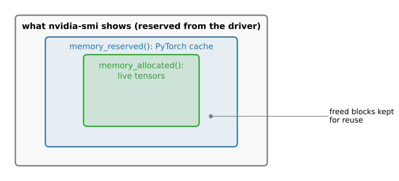
GPU allocators commonly retain freed blocks for reuse, so process-level memory reported by nvidia-smi can remain high after live tensors disappear. The durable distinction is between memory held by live arrays, memory reserved by a framework allocator, and memory reported for the whole process. The APIs below expose different layers of that accounting.
PyTorch uses a caching allocator: requesting memory from the CUDA driver is slow, so it uses a caching allocator: when a tensor dies, its block is not returned to the driver but kept in a per-process cache for the next tensor of a similar size. PyTorch therefore reports two numbers. torch.cuda.memory_allocated() counts bytes held by live tensors; torch.cuda.memory_reserved() counts those bytes plus the cache. nvidia-smi sees the process from the outside, so it reports roughly the reserved figure, which grows to the high-water mark of your program and stays there. Figure 5.7.2 shows how the three views nest inside one another.
On first use, TensorFlow may reserve a large fraction of GPU memory in one grab and hands out pieces of it from its own allocator; tf.config.experimental.set_memory_growth(gpu, True), called before the first computation, switches to growing the reservation on demand instead. nvidia-smi sees the process from the outside, so it reports the whole reservation no matter how little of it your tensors occupy. The real accounting lives inside: tf.config.experimental.get_memory_info('GPU:0') returns a dictionary whose 'current' entry counts live tensors and whose 'peak' entry is their high-water mark, the same nesting of views that Figure 5.7.2 sketches. There is no such allocator for the CPU, and the call raises on 'CPU:0'.
On first use, XLA commonly preallocates a configurable fraction of GPU memory and hands out pieces of it from its own allocator (the fraction is controlled by the XLA_PYTHON_CLIENT_PREALLOCATE and XLA_PYTHON_CLIENT_MEM_FRACTION environment variables). nvidia-smi sees the process from the outside, so it reports the whole preallocated block no matter how little of it your arrays occupy. The real accounting lives inside: device.memory_stats() returns a dictionary whose bytes_in_use entry counts live buffers and whose peak_bytes_in_use entry is their high-water mark, the same nesting of views that Figure 5.7.2 sketches. On the CPU backend there is no such allocator and the call returns None.
MXNet uses a device memory pool: requesting memory from the CUDA driver is slow, so it keeps a memory pool per device: when an array dies, its block is not returned to the driver but kept for the next array of a similar size, and nvidia-smi keeps counting it. MXNet 2.0 has no per-process counter of live bytes: the only built-in query is npx.gpu_memory_info(i), a wrapper around the driver’s cudaMemGetInfo that returns device-wide (free, total) bytes, the outermost of the three views in Figure 5.7.2 and the same number nvidia-smi prints. We can still watch the pool at work from the outside; gpu().empty_cache() releases its unreferenced blocks back to the driver.
if torch.cuda.is_available():
    def report(tag):
        print(f'{tag}: {torch.cuda.memory_allocated() / 2**20:7.1f} MiB '
              f'allocated, {torch.cuda.memory_reserved() / 2**20:7.1f} MiB '
              'reserved')
    big = torch.zeros(256, 1024, 1024, device=gpu())  # 1 GiB of float32
    report('after creating big')
    del big
    report('after deleting it ')
else:
    print('No CUDA device: both counters read 0 on the CPU.')
after creating big: 1032.1 MiB allocated, 1046.0 MiB reserved
after deleting it : 8.1 MiB allocated, 1046.0 MiB reservedif num_gpus() > 0:
def report(tag):
info = tf.config.experimental.get_memory_info('GPU:0')
print(f'{tag}: {info["current"] / 2**20:7.1f} MiB in use, '
f'{info["peak"] / 2**20:7.1f} MiB peak')
with gpu():
big = tf.zeros((256, 1024, 1024)) # 1 GiB of float32
report('after creating big')
del big
report('after deleting it ')
else:
print('No GPU: get_memory_info() tracks only GPU and TPU allocators.')after creating big: 1024.0 MiB in use, 1024.0 MiB peak
after deleting it : 0.0 MiB in use, 1024.0 MiB peakif num_gpus() > 0:
def report(tag):
s = gpu().memory_stats()
print(f'{tag}: {s["bytes_in_use"] / 2**20:7.1f} MiB in use, '
f'{s["peak_bytes_in_use"] / 2**20:7.1f} MiB peak')
big = jnp.zeros((256, 1024, 1024)) # 1 GiB of float32
big.block_until_ready()
report('after creating big')
del big
report('after deleting it ')
else:
print('No GPU: memory_stats() returns None on the CPU backend.')after creating big: 1024.0 MiB in use, 1024.0 MiB peak
after deleting it : 0.0 MiB in use, 1024.0 MiB peakif num_gpus() > 0:
def report(tag):
free, total = npx.gpu_memory_info(0)
print(f'{tag}: {(total - free) / 2**20:7.1f} MiB used on device 0')
report('baseline ')
big = np.zeros((256, 1024, 1024), ctx=gpu()) # 1 GiB of float32
npx.waitall()
report('after creating big')
del big
npx.waitall()
report('after deleting it ')
gpu().empty_cache()
report('after empty_cache ')
else:
print('No GPU: gpu_memory_info() queries the CUDA driver.')baseline : 886.4 MiB used on device 0
after creating big: 1910.4 MiB used on device 0
after deleting it : 1910.4 MiB used on device 0
after empty_cache : 886.4 MiB used on device 0After the deletion, memory_allocated() falls by a gibibyte while memory_reserved() does not move: the block went back to the cache, ready for reuse, and nvidia-smi keeps showing it. torch.cuda.empty_cache() returns the cached blocks to the driver, which is occasionally useful when another process needs the card, but do not call it inside a training loop: it forces the allocator to make slow driver requests all over again.
On a GPU, 'current' falls by a gibibyte the moment the last reference dies, while nvidia-smi does not move at all: the block returns to TensorFlow’s allocator pool, not to the driver. There is no empty_cache equivalent; the process keeps its reservation until it exits. If another process must share the card, enable memory growth, or set a hard cap with tf.config.set_logical_device_configuration, before the first computation.
On a GPU, bytes_in_use falls by a gibibyte the moment the buffer’s last reference dies, while nvidia-smi does not move at all: the block returns to XLA’s preallocated pool, not to the driver. If another process must share the card, set XLA_PYTHON_CLIENT_PREALLOCATE=false in the environment before the first computation; allocations then go to the driver on demand, visibly to nvidia-smi but more slowly.
The used figure jumps by a gibibyte when big is created and barely moves when it is deleted: the block went back to MXNet’s pool, not to the driver, and the driver-side view is all gpu_memory_info can see. Only empty_cache() makes the figure fall, and it frees just the pool’s unreferenced blocks. Two cautions: the reading is device-wide, so it includes the CUDA context and any other process on the card, which is why differences between readings are meaningful and absolute values are not; and do not call empty_cache inside a training loop, since it forces the pool to make slow driver requests all over again. The npx.waitall() before each reading matters too: MXNet executes asynchronously (more on this below), so without it we might read the driver’s counters before the allocation has happened.
5.7.2.1 What Fills Memory During Training
In Section 5.2 we did the bookkeeping on paper: a model with \(N\) parameters costs \(4N\) bytes for float32 weights, another \(4N\) for their gradients, and \(8N\) for Adam’s two moment estimates, roughly \(16N\) before any data arrives. The remaining term, the activations, is different in kind: backpropagation must remember the intermediate results of the forward pass in order to compute gradients, and their size scales with the batch size and with the width of every layer, while the \(16N\) does not.
We can watch each term arrive by reading memory_allocated() at four points of a single training step.
We can watch each term arrive by reading 'current' at four points of a single training step. The activations are visible as a plateau for the same reason as in PyTorch: tf.GradientTape records the forward pass and holds the intermediate results until we ask it for gradients.
We can watch the terms arrive by reading bytes_in_use around the pieces of a training step. The activations are the exception: they exist only while the gradient computation runs, so they leave their trace in peak_bytes_in_use rather than in a reading you can take afterwards.
MXNet cannot show the terms arriving one by one: with no per-process counter, gpu_memory_info sees only the device-wide total, and the pool’s high-water behavior smooths the individual plateaus out of that view, so the step-by-step readout in this subsection exists only in the other tabs. The accounting itself holds unchanged, with one timing difference: Gluon allocates each parameter’s gradient buffer at initialize time (and attach_grad does the same for from-scratch arrays), so the \(4N\) gradient term is resident from the start rather than appearing at the first backward pass. The device-wide counter supports the coarse before/after measurement above around a complete training step; the batch-size lesson at the end of this subsection applies in full.
if torch.cuda.is_available():
    def allocated():
        return f'{torch.cuda.memory_allocated() / 2**20:7.1f} MiB'
    net = nn.Sequential(nn.Linear(1024, 4096), nn.ReLU(),
                        nn.Linear(4096, 4096), nn.ReLU(),
                        nn.Linear(4096, 4096), nn.ReLU(),
                        nn.Linear(4096, 10)).to(gpu())
    opt = torch.optim.Adam(net.parameters())
    X = torch.randn(4096, 1024, device=gpu())
    y = torch.randint(0, 10, (4096,), device=gpu())
    print('weights           ', allocated())
    loss = F.cross_entropy(net(X), y)
    print('+ activations     ', allocated())
    loss.backward()
    print('+ gradients       ', allocated())
    opt.step()
    print('+ optimizer state ', allocated())
else:
    print('No CUDA device: run this cell on a GPU to see the four plateaus.')
weights 168.4 MiB
+ activations 361.5 MiB
+ gradients 321.7 MiB
+ optimizer state 610.1 MiBif num_gpus() > 0:
def in_use():
info = tf.config.experimental.get_memory_info('GPU:0')
return f'{info["current"] / 2**20:7.1f} MiB'
with gpu():
net = tf.keras.Sequential(
[tf.keras.layers.Dense(4096, activation='relu'),
tf.keras.layers.Dense(4096, activation='relu'),
tf.keras.layers.Dense(4096, activation='relu'),
tf.keras.layers.Dense(10)])
X = tf.random.normal((4096, 1024))
y = tf.random.uniform((4096,), 0, 10, dtype=tf.int32)
net(X) # The first call creates the variables
opt = tf.keras.optimizers.Adam()
loss_fn = tf.keras.losses.SparseCategoricalCrossentropy(from_logits=True)
print('weights ', in_use())
with tf.GradientTape() as tape:
loss = loss_fn(y, net(X, training=True))
print('+ activations ', in_use())
grads = tape.gradient(loss, net.trainable_variables)
print('+ gradients ', in_use())
opt.apply_gradients(zip(grads, net.trainable_variables))
print('+ optimizer state ', in_use())
else:
print('No GPU: run this cell on a GPU to see the four plateaus.')weights 160.2 MiB
+ activations 352.6 MiB
+ gradients 304.4 MiB
+ optimizer state 640.8 MiBif num_gpus() > 0:
def in_use():
s = gpu().memory_stats()
return f'{s["bytes_in_use"] / 2**20:7.1f} MiB'
rngs = nnx.Rngs(0)
net = nnx.Sequential(nnx.Linear(1024, 4096, rngs=rngs), nnx.relu,
nnx.Linear(4096, 4096, rngs=rngs), nnx.relu,
nnx.Linear(4096, 4096, rngs=rngs), nnx.relu,
nnx.Linear(4096, 10, rngs=rngs))
key1, key2 = jax.random.split(d2l.get_key())
X = jax.random.normal(key1, (4096, 1024))
y = jax.random.randint(key2, (4096,), 0, 10)
def loss(model):
logits = model(X)
return optax.softmax_cross_entropy_with_integer_labels(
logits, y).mean()
jax.block_until_ready(nnx.state(net))
print('weights ', in_use())
grads = jax.block_until_ready(nnx.grad(loss)(net))
print('+ gradients ', in_use())
optimizer = nnx.Optimizer(net, optax.adam(1e-3), wrt=nnx.Param)
jax.block_until_ready(optimizer.opt_state)
print('+ optimizer state ', in_use())
peak = gpu().memory_stats()['peak_bytes_in_use'] / 2**20
print(f'peak with activations {peak:7.1f} MiB')
else:
print('No GPU: run this cell on a GPU to see the terms arrive.')weights 160.2 MiB
+ gradients 304.4 MiB
+ optimizer state 592.9 MiB
peak with activations 1236.7 MiBThe four readings map onto the accounting. The first is the weights alone (about \(4N\) bytes, plus the input batch). The second jumps by the size of the stored activations — here roughly a third more than the weights; a larger batch or longer sequence scales this term while the weights stay put. The third falls back: backward frees the activations as it consumes them and leaves behind gradients exactly the size of the weights. The fourth adds \(8N\) at the first opt.step(), when Adam lazily creates its moment buffers. From then on the loop cycles between plateaus two and three; the weights, gradients, and optimizer state are permanent residents. Batch size is the first memory control to test because it scales activation memory without changing the model architecture. If a growing staircase appears across steps instead of this steady cycle, look for tensors that keep the computation graph alive between iterations, such as accumulating loss rather than loss.item() into a running total.
The four readings map onto the accounting. The first is the weights alone (about \(4N\) bytes, plus the input batch). The second jumps by the size of the activations the tape is holding — here roughly a third more than the weights; a larger batch or longer sequence scales this term while the weights stay put. The third falls back: tape.gradient consumes the recorded forward pass, frees it, and leaves behind gradients exactly the size of the weights. The fourth adds \(8N\) at the first apply_gradients, when Adam creates its slot variables. From then on the loop cycles between plateaus two and three; the weights, gradients, and optimizer state are permanent residents. Batch size is the first memory control to test because it scales activation memory without changing the model architecture. If a growing staircase appears across steps instead of this steady cycle, look for tensors kept alive between iterations, such as a Python list accumulating the loss tensor itself rather than float(loss), or a persistent GradientTape that remains active.
The readings map onto the accounting. The first is the weights alone (about \(4N\) bytes, plus the input batch). The second adds gradients exactly the size of the weights: in JAX a gradient is not a field attached to a parameter but a second pytree of the same shape, returned by jax.grad. The third adds \(8N\) when optax.adam’s init builds its two moment pytrees from the parameters, placed wherever they live. The activations never appear as a plateau: they exist only inside the jax.grad call, so the peak reading, several times the weights here because the batch is large, is the only evidence they leave. Batch size is the first memory control to test because it scales activation memory without changing the model architecture. If a growing staircase appears across steps, look for device arrays accumulating on the Python side, such as appending the loss array itself, rather than loss.item(), to a running log.
5.7.2.2 Trading Compute for Memory: Activation Checkpointing
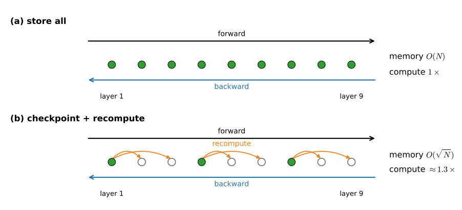
The activation term has a second knob. Backpropagation stores every intermediate result only to read each one exactly once, on the way back. Activation checkpointing (Chen et al. 2016) refuses to store them: it keeps only the inputs to selected segments of the network, and during the backward pass reruns each segment’s forward computation to regenerate the activations it needs. For a stack of \(N\) equally sized layers, dividing the stack into segments of about \(\sqrt{N}\) layers reduces stored activations from \(O(N)\) to \(O(\sqrt{N})\). Recomputing selected segments adds work, but the runtime overhead depends on segment size, operator mix, compiler, RNG handling, and hardware; it is not fixed by the asymptotic memory schedule. Figure 5.7.3 sketches this schedule. The trade pays off exactly where deep learning spends most of its time: deep stacks of identical blocks, such as the residual stack we assembled in Section 5.1 and every Transformer you will meet later. We rebuild a compact version of that block here.
class ResidualBlock(nn.Module):  # As in :numref:`sec_model_construction`
    def __init__(self, num_hiddens):
        super().__init__()
        self.body = nn.Sequential(
            nn.Linear(num_hiddens, num_hiddens), nn.ReLU(),
            nn.Linear(num_hiddens, num_hiddens), nn.ReLU())

    def forward(self, X):
        return X + self.body(X)

def run_stack(blocks, X, use_checkpoint=False, segment_size=4):
    for start in range(0, len(blocks), segment_size):
        stop = min(start + segment_size, len(blocks))
        def segment(X, start=start, stop=stop):
            for i in range(start, stop):
                X = blocks[i](X)
            return X
        X = checkpoint(segment, X, use_reentrant=False) \
            if use_checkpoint else segment(X)
    return X
class ResidualBlock(tf.keras.Model): # As in :numref:`sec_model_construction`
def __init__(self, num_hiddens):
super().__init__()
self.body = tf.keras.Sequential(
[tf.keras.layers.Dense(num_hiddens, activation='relu'),
tf.keras.layers.Dense(num_hiddens, activation='relu')])
def call(self, X):
return X + self.body(X)
def run_stack(blocks, X, use_checkpoint=False, segment_size=4):
for start in range(0, len(blocks), segment_size):
segment_blocks = blocks[start:start + segment_size]
def segment(X):
for blk in segment_blocks:
X = blk(X)
return X
f = tf.recompute_grad(segment) if use_checkpoint else segment
X = f(X)
return Xclass ResidualBlock(nnx.Module): # As in :numref:`sec_model_construction`
def __init__(self, num_hiddens, rngs):
self.body = nnx.Sequential(
nnx.Linear(num_hiddens, num_hiddens, rngs=rngs), nnx.relu,
nnx.Linear(num_hiddens, num_hiddens, rngs=rngs), nnx.relu)
def __call__(self, X):
return X + self.body(X)
def run_stack(graphdef, states, X, use_checkpoint=False, segment_size=4):
def segment(segment_states, X):
for state in segment_states:
X = nnx.merge(graphdef, state)(X)
return X
f = jax.checkpoint(segment) if use_checkpoint else segment
for start in range(0, len(states), segment_size):
X = f(states[start:start + segment_size], X)
return Xtorch.utils.checkpoint.checkpoint(segment, X) runs a segment without storing its internals and remembers just enough to recompute them later. Recomputation must reproduce the original forward pass bit for bit, so by default checkpoint also stashes and restores the random-number-generator state, which keeps segments containing dropout correct at a small extra cost (preserve_rng_state=False skips it for deterministic segments).
tf.recompute_grad(blk) returns a function that behaves exactly like blk on the forward pass but tells the tape to store only the inputs, rerunning blk during the backward pass to regenerate what it needs. One caveat: unlike its PyTorch counterpart it does not snapshot random-number state, so keep checkpointed segments deterministic (or drive their randomness with stateless seeds); a stateful dropout layer inside the segment can resample on recomputation.
jax.checkpoint (also exported as jax.remat) is a function transformation like grad and jit: jax.checkpoint(f) behaves exactly like f when called, but when differentiated it saves only f’s inputs and recomputes the internals during the backward pass. Randomness needs no special handling: JAX functions receive their PRNG keys as explicit arguments, so recomputation with the same key reproduces a segment containing dropout bit for bit by construction.
Activation checkpointing is not available in MXNet: neither mxnet.autograd nor Gluon offers a recompute-during-backward transform comparable to torch.utils.checkpoint, jax.checkpoint, or tf.recompute_grad, and none was added before development stopped. This subsection’s code therefore appears only in the supported tabs: the gradient-equality check and the peak-memory comparison below. Recomputation can cut activation memory in supported frameworks, with overhead that depends on the segmented computation. In MXNet the remaining memory knob demonstrated here is the batch size.
Before measuring memory, we should verify the claim that nothing about the result changes: the gradients through a checkpointed stack must equal the ordinary ones.
torch.manual_seed(0)
blocks = nn.Sequential(*[ResidualBlock(64) for _ in range(4)])
X = torch.randn(32, 64)

def stack_grads(use_checkpoint):
    blocks.zero_grad(set_to_none=True)
    run_stack(blocks, X, use_checkpoint).sum().backward()
    return [p.grad.clone() for p in blocks.parameters()]

for g, g_ckpt in zip(stack_grads(False), stack_grads(True)):
    assert torch.allclose(g, g_ckpt)
print('checkpointed gradients match the ordinary ones')
checkpointed gradients match the ordinary onestf.keras.utils.set_random_seed(0)
blocks = [ResidualBlock(64) for _ in range(4)]
X = tf.random.normal((32, 64))
def stack_grads(use_checkpoint):
with tf.GradientTape() as tape:
loss = tf.reduce_sum(run_stack(blocks, X, use_checkpoint))
params = [v for blk in blocks for v in blk.trainable_variables]
return tape.gradient(loss, params)
for g, g_ckpt in zip(stack_grads(False), stack_grads(True)):
assert np.allclose(g, g_ckpt)
print('checkpointed gradients match the ordinary ones')checkpointed gradients match the ordinary onesX = jax.random.normal(jax.random.key(1), (32, 64))
blocks = [ResidualBlock(64, nnx.Rngs(k))
for k in jax.random.split(jax.random.key(0), 4)]
split_blocks = [nnx.split(block) for block in blocks]
graphdef = split_blocks[0][0]
states = [state for _, state in split_blocks]
def stack_grads(use_checkpoint):
loss = lambda states: run_stack(graphdef, states, X,
use_checkpoint).sum()
return jax.tree_util.tree_leaves(jax.grad(loss)(states))
for g, g_ckpt in zip(stack_grads(False), stack_grads(True)):
assert jnp.allclose(g, g_ckpt)
print('checkpointed gradients match the ordinary ones')checkpointed gradients match the ordinary onesThat check runs anywhere, CPU included. The memory effect needs a GPU and a stack deep enough for the difference to be unambiguous: sixteen blocks of width 1024 at batch size 8192.
if torch.cuda.is_available():
    blocks = nn.Sequential(*[ResidualBlock(1024) for _ in range(16)]).to(gpu())
    X = torch.randn(8192, 1024, device=gpu())
    for use_checkpoint in (False, True):
        blocks.zero_grad(set_to_none=True)
        torch.cuda.synchronize()
        torch.cuda.reset_peak_memory_stats()
        t = time.time()
        run_stack(blocks, X, use_checkpoint).sum().backward()
        torch.cuda.synchronize()
        print(f'checkpointing={use_checkpoint!s:5}  peak '
              f'{torch.cuda.max_memory_allocated() / 2**20:6.0f} MiB, '
              f'{time.time() - t:.2f} sec')
else:
    print('No CUDA device: peak-memory comparison needs a GPU.')
checkpointing=False peak 2358 MiB, 0.04 sec
checkpointing=True peak 1335 MiB, 0.05 secif num_gpus() > 0:
with gpu():
blocks = [ResidualBlock(1024) for _ in range(16)]
X = tf.random.normal((8192, 1024))
run_stack(blocks, X) # Create the variables before measuring
params = [v for blk in blocks for v in blk.trainable_variables]
for use_checkpoint in (False, True):
tf.config.experimental.reset_memory_stats('GPU:0')
t = time.time()
with tf.GradientTape() as tape:
loss = tf.reduce_sum(run_stack(blocks, X, use_checkpoint))
grads = tape.gradient(loss, params)
tf.test.experimental.sync_devices()
peak = tf.config.experimental.get_memory_info('GPU:0')['peak'] / 2**20
print(f'checkpointing={use_checkpoint!s:5} peak {peak:6.0f} MiB, '
f'{time.time() - t:.2f} sec')
else:
print('No GPU: peak-memory comparison needs a GPU.')checkpointing=False peak 2509 MiB, 0.09 sec
checkpointing=True peak 1521 MiB, 0.16 secif num_gpus() > 0:
X = jax.random.normal(jax.random.key(1), (8192, 1024))
blocks = [ResidualBlock(1024, nnx.Rngs(k))
for k in jax.random.split(jax.random.key(0), 16)]
split_blocks = [nnx.split(block) for block in blocks]
graphdef = split_blocks[0][0]
states = [state for _, state in split_blocks]
for use_checkpoint in (True, False): # low first: the peak only grows
grad_fn = jax.jit(jax.grad(
lambda states: run_stack(
graphdef, states, X, use_checkpoint).sum()))
jax.block_until_ready(grad_fn(states)) # compile outside timing
t = time.time()
jax.block_until_ready(grad_fn(states))
peak = gpu().memory_stats()['peak_bytes_in_use'] / 2**20
print(f'checkpointing={use_checkpoint!s:5} peak {peak:6.0f} MiB, '
f'{time.time() - t:.2f} sec')
else:
print('No GPU: peak-memory comparison needs a GPU.')checkpointing=True peak 1377 MiB, 0.07 sec
checkpointing=False peak 2401 MiB, 0.06 secWithout checkpointing, the peak includes activations from all sixteen blocks. With four-block segments, it includes the four segment inputs plus the recomputed activations of one segment, at the cost of a slower step. This tradeoff can enable training when stored activations would otherwise exceed device memory, and it is widely used in large Transformer training runs.
5.7.3 Asynchronous Execution and Input Transfer
Accelerator work is usually queued asynchronously: Python can return from an operation before the device finishes it. Accurate timing therefore requires a warm-up followed by an explicit synchronization, while frequent scalar reads, logging, or host conversions can serialize the pipeline. The backend-specific difference is the synchronization primitive and whether CPU dispatch is also asynchronous.
CUDA operations are asynchronous with respect to Python; use torch.cuda.synchronize() around a timed region. CPU operations here are synchronous.
GPU kernels and traced graphs can be dispatched asynchronously. In these examples tf.test.experimental.sync_devices() supplies the explicit barrier; eager CPU operations are synchronous.
JAX dispatch may be asynchronous on CPU and GPU. Call block_until_ready() on the result before stopping a timer.
MXNet’s engine is asynchronous on CPU and GPU. npx.waitall() blocks until queued operations finish and is the synchronization primitive used for timing.
if torch.cuda.is_available():
    A = torch.randn(4096, 4096, device=gpu())
    torch.cuda.synchronize()
    t = time.time()
    for _ in range(32):
        B = A @ A
    print(f'time to queue 32 matrix products: {time.time() - t:.4f} sec')
    torch.cuda.synchronize()
    print(f'time until they all finished:     {time.time() - t:.4f} sec')
else:
    print('No CUDA device: CPU operations run synchronously.')
time to queue 32 matrix products: 0.0014 sec
time until they all finished: 0.0801 secif num_gpus() > 0:
with gpu():
A = tf.random.normal((4096, 4096))
(A @ A).numpy() # Warm up
t = time.time()
for _ in range(32):
B = A @ A
print(f'time to queue 32 matrix products: {time.time() - t:.4f} sec')
tf.test.experimental.sync_devices()
print(f'time until they all finished: {time.time() - t:.4f} sec')
else:
print('No GPU: TensorFlow executes CPU ops synchronously.')time to queue 32 matrix products: 0.0027 sec
time until they all finished: 0.0538 secA = jax.random.normal(jax.random.key(0), (2000, 2000)) / 45
(A @ A).block_until_ready() # Warm up
B, t = A, time.time()
for _ in range(32):
B = B @ A # Chained, so the last result implies all finished
print(f'time to queue 32 matrix products: {time.time() - t:.4f} sec')
B.block_until_ready()
print(f'time until they all finished: {time.time() - t:.4f} sec')time to queue 32 matrix products: 0.0028 sec
time until they all finished: 0.0159 secA = np.random.normal(size=(1000, 1000))
B = np.dot(A, A)
npx.waitall() # Warm up
t = time.time()
for _ in range(32):
B = np.dot(A, A)
print(f'time to queue 32 matrix products: {time.time() - t:.4f} sec')
npx.waitall()
print(f'time until they all finished: {time.time() - t:.4f} sec')time to queue 32 matrix products: 0.0014 sec
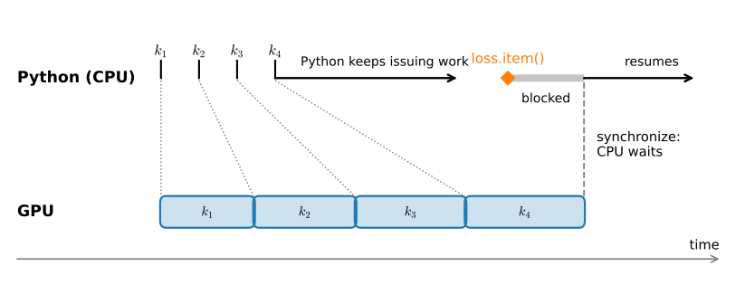
time until they all finished: 0.4117 secPython returned from the loop in a few milliseconds; the products were still running. Any operation that needs a concrete value on the host forces a synchronization point: .item(), .numpy(), print, an if on a tensor’s value. Each one makes Python block until the queue drains, and the device then sits idle until Python catches up. A print(loss.item()) in the inner loop can serialize the whole pipeline this way, once per step, as Figure 5.7.4 lays out. The fix is not to give up monitoring but to move it off the hot path: keep running statistics on the device and transfer them once per epoch, or hand values to a background consumer, which is exactly what our ProgressBoard from Section 2.2 does when the Trainer plots the loss.
Python returned from the loop in a few milliseconds; the products were still running. Any operation that needs a concrete value on the host forces a synchronization point: .numpy(), float(loss), print, an if on a tensor’s value. Each one makes Python block until the queue drains, and the device then sits idle until Python catches up (tf.test.experimental.sync_devices() is the explicit version that accurate timings need). A print(float(loss)) in the inner loop can serialize the whole pipeline this way, once per step, as Figure 5.7.4 lays out. The fix is not to give up monitoring but to move it off the hot path: keep running statistics on the device and transfer them once per epoch, or hand values to a background consumer, which is exactly what our ProgressBoard from Section 2.2 does when the Trainer plots the loss.
Python returned from the loop in a few milliseconds — far less time than the 32 matrix products take; they were still running. Any operation that needs a concrete value on the host forces a synchronization point: .item(), np.asarray, print, an if on an array’s value, and block_until_ready() itself, whose job is to make the synchronization explicit (our timings above depend on it). Each one makes Python block until the queued work drains, and the device then sits idle until Python catches up. A print(loss.item()) in the inner loop can serialize the whole pipeline this way, once per step, as Figure 5.7.4 lays out. The fix is not to give up monitoring but to move it off the hot path: keep running statistics on the device and transfer them once per epoch, or hand values to a background consumer, which is exactly what our ProgressBoard from Section 2.2 does when the Trainer plots the loss.
Python returned from the loop in a few milliseconds; the products were still running. Any operation that needs a concrete value on the host forces a synchronization point: asnumpy(), .item(), print, an if on a tensor’s value. Each one makes Python block until the engine has produced that value, and the backend then sits idle until Python catches up (npx.waitall() is the explicit, drain-everything version that accurate timings need). A print(loss.item()) in the inner loop can serialize the whole pipeline this way, once per step, as Figure 5.7.4 lays out; worse, the conversion to NumPy holds Python’s global interpreter lock while it waits. The fix is not to give up monitoring but to move it off the hot path: keep running statistics on the device and transfer them once per epoch, or hand values to a background consumer. In MXNet, our ProgressBoard from Section 2.2 can take over only the drawing. Module.plot still converts the loss to NumPy on the training thread at every step, because MXNet’s engine is not safe for GPU-to-host transfers issued from another thread.
The same overlap idea applies to getting data onto the device. An ordinary host-to-device copy must first move the batch into non-pageable (“pinned”) memory that the DMA engine can read, then transfer it, and the call blocks Python throughout. If the source already sits in pinned memory, the copy can be issued with non_blocking=True and Python continues immediately, preparing the next batch while the transfer overlaps the GPU’s current work.
The same overlap idea applies to getting data onto the device, and in TensorFlow it belongs to the input pipeline rather than to a per-tensor flag: ending a tf.data pipeline with .prefetch(tf.data.AUTOTUNE) keeps the next batches being prepared in the background while the device computes, and tf.data.experimental.prefetch_to_device stages them on the GPU ahead of use. The book’s data loaders are tf.data.Datasets, so this section’s overlap discipline reduces to one appended call. The full treatment of asynchrony, streams, and multi-device parallelism is in Chapter 13.
The same overlap idea applies to getting data onto the device, and in JAX it needs no per-tensor flag: device_put dispatches the transfer and returns immediately, so Python prepares the next batch while the copy overlaps the device’s current work, which is exactly the effect other stacks arrange with pinned host buffers. The full treatment of asynchrony, streams, and multi-device parallelism is in Chapter 13.
The same overlap idea applies to getting data onto the device. MXNet makes page-locked host memory a device in its own right: an array created with ctx=npx.cpu_pinned() lives in memory the DMA engine can read directly, so its copy to the GPU is faster than one from pageable memory, and Gluon’s DataLoader(pin_memory=True) stages every batch there for you. The copy itself needs no per-tensor flag: copyto is an engine operation like any other, dispatched asynchronously, so Python is free to prepare the next batch while it runs. The full treatment of asynchrony, streams, and multi-device parallelism is in Chapter 13.
if torch.cuda.is_available():
    x = torch.randn(16, 3, 224, 224)  # A typical image batch
    x_pinned = x.pin_memory()
    def copy_time(src, non_blocking=False, n=100):
        torch.cuda.synchronize()
        t = time.time()
        for _ in range(n):
            src.to(gpu(), non_blocking=non_blocking)
        torch.cuda.synchronize()
        return (time.time() - t) / n * 1e3
    print(f'pageable copy:              {copy_time(x):.3f} ms')
    print(f'pinned, non-blocking copy:  {copy_time(x_pinned, True):.3f} ms')
else:
    print('No CUDA device: host-to-device copies do not arise.')
pageable copy: 0.521 ms
pinned, non-blocking copy: 0.408 msTwo caveats matter. Pinning is itself expensive, so synchronously pinning a tensor on the training thread just before one copy can erase the benefit. DataLoader(pin_memory=True) performs the pinning in its input pipeline, while non_blocking=True lets the training thread enqueue the transfer without waiting; this is why the two options are the standard pairing. A non-blocking copy may still be in progress when the call returns. Mutating the source CPU tensor before the transfer finishes can change the data received by the device. The full treatment of asynchrony, streams, and multi-device parallelism is in Chapter 13.
5.7.4 Device-Aware Trainer
In Section 2.2 the Trainer accepted a num_gpus argument and did not use it. The implementation now applies the placement rules from this section: the model moves to the device once, before training, and every batch streams over per step, at the boundary of the computation.
In Section 2.2 the Trainer accepted a num_gpus argument and did not use it. The implementation now applies the placement rules from this section: the model’s variables are created on the device by a first forward pass (which the Trainer already runs before training, when it compiles its step functions), and every batch is re-materialized on the device per step, at the boundary of the computation.
In Section 2.2 the Trainer accepted a num_gpus argument and did not use it. The implementation now applies the placement rules from this section: the parameters are created on the accelerator once, before training (JAX initializes arrays on the default device, which is the accelerator whenever one exists), and every batch streams over per step, at the boundary of the computation.
In Section 2.2 the Trainer accepted a num_gpus argument and did not use it. The implementation now applies the placement rules from this section: the model’s parameters are re-assigned to the device once, before training (reset_ctx, which works even while Gluon’s parameters are still waiting for their shapes), and every batch streams over per step, at the boundary of the computation.
@d2l.add_to_class(d2l.Trainer)
def __init__(self, max_epochs, num_gpus=0, gradient_clip_val=0):
    self.save_hyperparameters()
    self.gpus = [d2l.gpu(i) for i in range(min(num_gpus, d2l.num_gpus()))]

@d2l.add_to_class(d2l.Trainer)
def prepare_batch(self, batch):
    if self.gpus:
        batch = [d2l.to(a, self.gpus[0]) for a in batch]
    return batch

@d2l.add_to_class(d2l.Trainer)
def prepare_model(self, model):
    model.trainer = self
    model.board.xlim = [0, self.max_epochs]
    if self.gpus:
        model.to(self.gpus[0])
self.model = model@d2l.add_to_class(d2l.Trainer)
def __init__(self, max_epochs, num_gpus=0, gradient_clip_val=0):
self.save_hyperparameters()
self.gpus = [d2l.gpu(i) for i in range(min(num_gpus, d2l.num_gpus()))]
@d2l.add_to_class(d2l.Trainer)
def prepare_batch(self, batch):
if self.gpus:
# tf.data.Dataset emits batches on CPU. Re-wrap them inside the
# GPU device context so subsequent ops keep their inputs on-device
# rather than incurring an implicit copy each step.
with self.gpus[0]:
batch = [tf.identity(a) for a in batch]
return batch@d2l.add_to_class(d2l.Trainer)
def __init__(self, max_epochs, num_gpus=0, gradient_clip_val=0):
self.save_hyperparameters()
self.gpus = [d2l.gpu(i) for i in range(min(num_gpus, d2l.num_gpus()))]
@d2l.add_to_class(d2l.Trainer)
def prepare_batch(self, batch):
if self.gpus:
batch = [d2l.to(a, self.gpus[0]) for a in batch]
return batch@d2l.add_to_class(d2l.Trainer)
def __init__(self, max_epochs, num_gpus=0, gradient_clip_val=0):
self.save_hyperparameters()
self.gpus = [d2l.gpu(i) for i in range(min(num_gpus, d2l.num_gpus()))]
@d2l.add_to_class(d2l.Trainer)
def prepare_batch(self, batch):
if self.gpus:
batch = [d2l.to(a, self.gpus[0]) for a in batch]
return batch
@d2l.add_to_class(d2l.Trainer)
def prepare_model(self, model):
model.trainer = self
model.board.xlim = [0, self.max_epochs]
if self.gpus:
model.reset_ctx(self.gpus[0])
model.set_scratch_params_device(self.gpus[0])
self.model = modelThe min(num_gpus, d2l.num_gpus()) makes the request a ceiling rather than a demand: on a machine with no GPU, self.gpus is empty, both hooks become no-ops, and training proceeds on the CPU. Every Trainer(num_gpus=1) you see from the next chapter onward relies on this fallback, which is how one codebase serves both the laptop you are reading on and a GPU server. As a capstone we train a classifier built from this chapter’s residual blocks on Fashion-MNIST; the Trainer places the model, moves each batch, and the memory budget of the run is exactly the four-plateau accounting from above.
The min(num_gpus, d2l.num_gpus()) makes the request a ceiling rather than a demand: on a machine with no GPU, self.gpus is empty, prepare_batch is a no-op, and training proceeds on the CPU. The explicit tf.identity inside the device scope matters because tf.data pipelines emit their batches on the CPU: without it, every op that touches the batch pays the silent host-to-device copy this section warned about, once per step. There is no prepare_model patch to write, since Keras variables are created on the first call and the Trainer runs its compile-time forward pass through prepare_batch, so the weights land on the configured GPU automatically. Every Trainer(num_gpus=1) you see from the next chapter onward relies on this fallback, which is how one codebase serves both the laptop you are reading on and a GPU server. As a capstone we train a classifier built from this chapter’s residual blocks on Fashion-MNIST; the memory budget of the run is exactly the four-plateau accounting from above.
The min(num_gpus, d2l.num_gpus()) makes the request a ceiling rather than a demand: on a machine with no GPU, self.gpus is empty, prepare_batch is a no-op, and training proceeds on the CPU. There is no model hook to patch, because fit initializes the parameters itself and JAX creates them on the default device, the GPU whenever one is present. Every Trainer(num_gpus=1) you see from the next chapter onward relies on this fallback, which is how one codebase serves both the laptop you are reading on and a GPU server. As a capstone we train a classifier built from this chapter’s residual blocks on Fashion-MNIST; the Trainer moves each batch, and the memory budget of the run is exactly the accounting from above.
The min(num_gpus, d2l.num_gpus()) makes the request a ceiling rather than a demand: on a machine with no GPU, self.gpus is empty, both hooks become no-ops, and training proceeds on the CPU. Every Trainer(num_gpus=1) you see from the next chapter onward relies on this fallback, which is how one codebase serves both the laptop you are reading on and a GPU server. As a capstone we train a classifier built from residual blocks on Fashion-MNIST; since the checkpointing comparison above has no MXNet variant, we define the Gluon rendition of Section 5.1’s block here. The Trainer re-assigns the parameters once, moves each batch, and the memory budget of the run follows the accounting from above.
class ResMLPClassifier(d2l.Classifier):
    def __init__(self, num_hiddens=256, num_blocks=2, lr=0.1):
        super().__init__()
        self.save_hyperparameters()
        self.net = nn.Sequential(
            nn.Flatten(), nn.LazyLinear(num_hiddens), nn.ReLU(),
            *[ResidualBlock(num_hiddens) for _ in range(num_blocks)],
            nn.LazyLinear(10))

trainer = d2l.Trainer(max_epochs=1, num_gpus=1)
trainer.fit(ResMLPClassifier(), d2l.FashionMNIST(batch_size=256))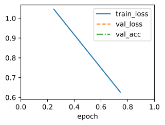
class ResMLPClassifier(d2l.Classifier):
    def __init__(self, num_hiddens=256, num_blocks=2, lr=0.1):
        super().__init__()
        self.save_hyperparameters()
        self.net = tf.keras.Sequential(
            [tf.keras.layers.Flatten(),
             tf.keras.layers.Dense(num_hiddens, activation='relu'),
             *[ResidualBlock(num_hiddens) for _ in range(num_blocks)],
             tf.keras.layers.Dense(10)])

trainer = d2l.Trainer(max_epochs=1, num_gpus=1)
trainer.fit(ResMLPClassifier(), d2l.FashionMNIST(batch_size=256))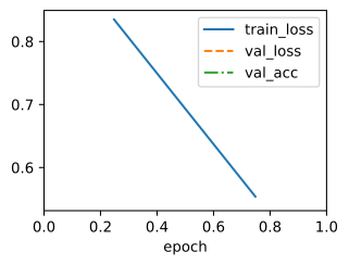
class ResMLPClassifier(d2l.Classifier):
    def __init__(self, num_hiddens=256, num_blocks=2, lr=0.1, rngs=None):
        super().__init__()
        self.save_hyperparameters(ignore=['rngs'])
        rngs = nnx.Rngs(0) if rngs is None else rngs
        self.net = nnx.Sequential(
            lambda x: x.reshape((x.shape[0], -1)),
            nnx.Linear(784, num_hiddens, rngs=rngs), nnx.relu,
            *[ResidualBlock(num_hiddens, rngs) for _ in range(num_blocks)],
            nnx.Linear(num_hiddens, 10, rngs=rngs))

trainer = d2l.Trainer(max_epochs=1, num_gpus=1)
trainer.fit(ResMLPClassifier(), d2l.FashionMNIST(batch_size=256))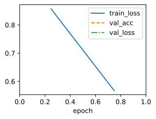
@d2l.add_to_class(d2l.Module)
def set_scratch_params_device(self, device):
    for attr in dir(self):
        a = getattr(self, attr)
        if isinstance(a, np.ndarray):
            setattr(self, attr, a.as_in_ctx(device))
            getattr(self, attr).attach_grad()
        if isinstance(a, d2l.Module):
            a.set_scratch_params_device(device)
        if isinstance(a, list):
            for elem in a:
elem.set_scratch_params_device(device)class ResidualBlock(nn.Block): # As in :numref:`sec_model_construction`
def __init__(self, num_hiddens):
super().__init__()
self.body = nn.Sequential()
self.body.add(nn.Dense(num_hiddens, activation='relu'),
nn.Dense(num_hiddens, activation='relu'))
def forward(self, X):
return X + self.body(X)
class ResMLPClassifier(d2l.Classifier):
def __init__(self, num_hiddens=256, num_blocks=2, lr=0.1):
super().__init__()
self.save_hyperparameters()
self.net = nn.Sequential()
self.net.add(nn.Dense(num_hiddens, activation='relu'),
*[ResidualBlock(num_hiddens) for _ in range(num_blocks)],
nn.Dense(10))
self.net.initialize()
trainer = d2l.Trainer(max_epochs=1, num_gpus=1)
trainer.fit(ResMLPClassifier(), d2l.FashionMNIST(batch_size=256))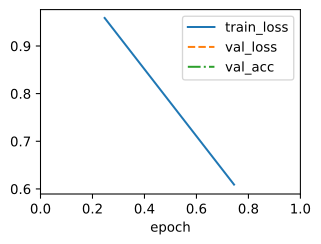
5.7.5 Summary
Every tensor and every parameter lives on a device, and operations combine only co-located tensors; copies between devices are explicit (.to), can dominate short computations, and belong at the boundary of the training loop rather than inside it. The principal GPU-memory terms during training are weights, gradients, optimizer state (fixed by the model and optimizer), and activations (scaling with batch size); memory_allocated() tracks live tensors while nvidia-smi shows the caching allocator’s high-water mark, so the two disagree by design. Activation checkpointing recomputes instead of storing selected activations; its runtime overhead is configuration-dependent. The GPU runs asynchronously ahead of Python: .item(), .numpy(), and print are synchronization points that stall the pipeline, and pinned memory with non_blocking=True lets transfers overlap compute. The Trainer encodes the placement discipline: model moved once, batches moved per step, graceful CPU fallback when no GPU exists.
Every tensor and every Keras variable lives on a device, and TensorFlow’s silent device policy will copy across devices for you, so keeping copies explicit and at the boundary of the training loop is a discipline here rather than an enforced rule; it matters just as much, because the hidden transfer has the same communication cost. The principal GPU-memory terms during training are: weights, gradients, optimizer state (fixed by the model and optimizer), and the activations the GradientTape records (scaling with batch size); get_memory_info tracks live tensors inside the reservation TensorFlow maps at startup, while nvidia-smi shows the whole reservation, so the two disagree by design. Activation checkpointing (tf.recompute_grad) recomputes instead of storing selected activations, with configuration-dependent runtime overhead. On a GPU, eager kernels run asynchronously ahead of Python: .numpy(), float(), and print are synchronization points that stall the pipeline, and .prefetch(tf.data.AUTOTUNE) is where input transfer overlaps compute. The Trainer encodes the placement discipline: variables created on the device at the compile-time forward pass, batches re-wrapped per step, graceful CPU fallback when no GPU exists.
Every array and every parameter lives on a device, and committed arrays combine only when co-located; copies between devices are explicit (device_put), can dominate short computations, and belong at the boundary of the training loop rather than inside it. The principal GPU-memory terms during training are weights, gradients, optimizer state (fixed by the model and optimizer), and activations (scaling with batch size); device.memory_stats() tracks live buffers inside the block XLA preallocates, while nvidia-smi shows the whole block, so the two disagree by design. Activation checkpointing (jax.checkpoint) recomputes instead of storing selected activations, with configuration-dependent overhead. Dispatch is asynchronous on every backend: .item(), np.asarray, and print are synchronization points that stall the pipeline, and block_until_ready() is the explicit one that accurate timings need. The Trainer encodes the placement discipline: parameters created on the device once, batches moved per step, graceful CPU fallback when no GPU exists.
Every tensor and every parameter lives on a device (MXNet 2.0’s name for the 1.x context), and operations combine only co-located tensors; copies between devices are explicit (copyto, or the no-op-when-possible as_in_ctx), can dominate short computations, and belong at the boundary of the training loop rather than inside it. The principal GPU-memory terms during training are weights, gradients, optimizer state (fixed by the model and optimizer), and activations (scaling with batch size); MXNet has no per-process counter for them, only the device-wide gpu_memory_info, and no activation-checkpointing utility. In these examples, batch size is the main control over activation memory; architecture and numeric precision also affect total memory. The execution engine is asynchronous on every backend: asnumpy(), .item(), and print are synchronization points that stall the pipeline, and npx.waitall() is the explicit one that accurate timings need. The Trainer encodes the placement discipline: parameters re-assigned once, batches moved per step, graceful CPU fallback when no GPU exists.
5.7.6 Exercises
- [code] Peak memory. Take a four-layer MLP with widths 1024, 4096, 4096, 4096 and 10 outputs, trained with Adam, as in Section 5.7.2.1. Using the accounting of that subsection, predict the peak memory of one training step at batch sizes 64, 256, and 1024, counting weights, gradients, optimizer state, and the activations the backward pass keeps. Then measure the peak on a GPU. Where does the prediction break down, and what did it omit?
- [code] Activation checkpointing. Revisit the comparison of
Section 5.7.2.2.
- Increase the batch size until the run without checkpointing raises an out-of-memory error. How much further can the checkpointed run go before it does too? Explain the ratio from what each variant stores.
- Run
run_stackwithsegment_sizeequal to 1, 4, and the number of blocks, and once without checkpointing. Plot peak memory against step time for the four configurations. Which segment size would you choose here, and why?
- [code] Activation checkpointing. Revisit the comparison of
Section 5.7.2.2.
- Increase the batch size until the run without checkpointing raises an out-of-memory error. How much further can the checkpointed run go before it does too? Explain the ratio from what each variant stores.
- Run
run_stackwithsegment_sizeequal to 1, 4, and the number of blocks, and once without checkpointing. Plot peak memory against step time for the four configurations. Which segment size would you choose here, and why?
- [code] Activation checkpointing. Revisit the comparison of
Section 5.7.2.2.
- Increase the batch size until the run without checkpointing raises an out-of-memory error. How much further can the checkpointed run go before it does too? Explain the ratio from what each variant stores.
- Run
run_stackwithsegment_sizeequal to 1, 4, and the number of blocks, and once without checkpointing. Run each configuration in a fresh process, becausepeak_bytes_in_usenever decreases within one. Plot peak memory against step time for the four configurations. Which segment size would you choose here, and why?
- Checkpointing arithmetic. MXNet has no recompute-during-backward transform, so work out the schedule of Figure 5.7.3 on paper for a stack of sixteen
ResidualBlocks of width 1024 at batch size 8192.- Name the arrays inside one block that the backward pass must keep, and count their entries.
- Compute the activation memory held at the peak of the backward pass without checkpointing and with segments of one, two, four, and eight blocks. State how much forward computation each schedule repeats.
- Which segment size would you choose here, and how does it relate to the rule of segments of about \(\sqrt{N}\) layers in Section 5.7.2.2?
[code] Synchronization points. ● Consider the training run of
ResMLPClassifierin Section 5.7.4 on a GPU.- List every synchronization point in one training step, reading
Trainer.fit_epoch,Trainer.prepare_batch, andModule.plotas well as the model code. Classify each as unavoidable for a correct loop or as an avoidable instrumentation artifact, and justify each classification. - Suppose the loop reads the loss into a Python float after every step. Predict from your list how much this readout slows down the default
ResMLPClassifierandResMLPClassifier(num_hiddens=2048, num_blocks=8). Then time one epoch of each model with and without the readout, and explain the four timings.
Adapted from the PyTorch documentation CUDA semantics.
- List every synchronization point in one training step, reading
[code] Asynchronous dispatch. ● Use the warm-up-then-synchronize timing pattern of Section 5.7.3 for both parts.
- For \(n\) from 256 to 8192, time a round trip of an \(n \times n\) matrix from CPU to GPU and back, and time one \(n \times n\) matrix product on the device. Find the \(n\) at which the two times are equal, extrapolating from how each time grows with \(n\) if they do not cross in this range. Predict this crossover from your GPU’s published host-to-device bandwidth and matrix-product throughput, and explain any gap between prediction and measurement.
- If you have two GPUs, time 1000 matrix products of two \(4096 \times 4096\) matrices executed on one GPU, then 500 on each of two GPUs issued from the same loop. Measure the scaling, explain how asynchronous dispatch lets Python issue work to both devices, and identify sources of deviation from linear scaling. Guard the experiment with
num_gpus() >= 2.
[code] Precision crossover. ● Run the
trainfunction of Section 5.5 on a GPU, with the network, every batch, and the 16-bit compute all placed on the device, and give it the hidden width and the batch size as arguments. Time its fp32 and mixed-precision runs with the warm-up-then-synchronize pattern of Section 5.7.3: at every setting, run one untimed warm-up step and then time ten steps.- For hidden widths 256 and 4096, sweep the batch size from 8 to 4096 in powers of two and plot the mixed-precision speedup over fp32 against the batch size, one curve per width.
- Below which batch size, if any, is mixed precision slower than fp32 at each width? Explain the reversal and why the crossover moves with the width.
Adapted from the PyTorch recipe Automatic Mixed Precision.