torch.set_float32_matmul_precision('high') # tf32 matmuls on tensor cores17.4 Samplers, Inversion and Editing
Every step of a sampler costs one evaluation of the U-Net, and the ancestral chain of Section 17.2 takes a thousand steps per image. The last section sampled with fifty Euler steps of the probability-flow ODE, and on its conditional model the thousand-step chain scored only a little lower in FD, at twenty times the evaluations. Which of the thousand steps do we need, and how few can we take? And once sampling is the integration of a field, can we run it backwards, from a real image to the noise that produces it, and edit the image from there?
J. Song et al. (2021) answered the first question with an observation about training. The regression of Section 17.2 sees single noisy points \(\mathbf{x}_t\) of training examples, never a chain of them, so it determines the distribution of \(\mathbf{x}_t\) at each time and nothing more. Many samplers produce those distributions, among them a deterministic one that takes long strides and can be run in reverse, and one trained network serves all of them. Karras et al. (2022) read the deterministic sampler as a numerical method for a differential equation, separating two choices that earlier samplers had made together: the order of the method and the placement of its steps. Meng et al. (2022) used the reverse direction to edit images.
We derive the family of samplers and its deterministic member, Euler’s method, measure quality against evaluations on the mixture and on Fashion-MNIST, and end with inversion, editing and inpainting.
17.4.1 One Field, Two Samplers
The ancestral chain and Euler’s method of Section 17.2, one adding fresh noise at every step and the other none, read the network through the same pair of estimates: at a point \(\mathbf{x}_t = \alpha_t \mathbf{x}_0 + \sigma_t \boldsymbol\epsilon\) of a Gaussian path, the clean point \(\hat{\mathbf{x}}_0\) and the noise \(\hat{\boldsymbol\epsilon}\), each of which determines the other:
\[\hat{\mathbf{x}}_0 = \frac{\mathbf{x}_t - \sigma_t \hat{\boldsymbol\epsilon}}{\alpha_t}. \tag{17.4.1}\]
Whatever the network was trained to predict, d2l.make_pred of Section 17.2 turns it into a function pred(x, alpha, sigma) returning this pair at any noise level, and the samplers of this section read nothing else.
17.4.1.1 The DDIM Family and Euler’s Method
Take a time \(t\) and an earlier time \(s < t\). A sampler step from \(t\) to \(s\) must turn a point distributed like \(\mathbf{x}_t\) into one distributed like \(\mathbf{x}_s\); the regression constrains nothing else. Write \(\mathbf{x}_t = \alpha_t \mathbf{x}_0 + \sigma_t \boldsymbol\epsilon\), choose a noise scale \(\tilde\sigma\) between \(0\) and \(\sigma_s\), and set
\[\mathbf{x}_s = \alpha_s \mathbf{x}_0 + \sqrt{\sigma_s^2 - \tilde\sigma^2}\, \boldsymbol\epsilon + \tilde\sigma\, \boldsymbol\xi, \qquad \boldsymbol\xi \sim \mathcal{N}(\mathbf{0}, \mathbf{I}), \tag{17.4.2}\]
with \(\boldsymbol\xi\) independent of \(\boldsymbol\epsilon\). The two noise variances add to \(\sigma_s^2\), so given \(\mathbf{x}_0\) the point \(\mathbf{x}_s\) has its correct distribution for every \(\tilde\sigma\), and since \(\boldsymbol\epsilon = (\mathbf{x}_t - \alpha_t \mathbf{x}_0) / \sigma_t\), each \(\tilde\sigma\) defines a step from \(\mathbf{x}_t\) to \(\mathbf{x}_s\). A sampler uses the network’s estimates in place of \(\mathbf{x}_0\) and \(\boldsymbol\epsilon\):
\[\mathbf{x}_s = \alpha_s \hat{\mathbf{x}}_0 + \sqrt{\sigma_s^2 - \tilde\sigma^2}\, \hat{\boldsymbol\epsilon} + \tilde\sigma\, \boldsymbol\xi. \tag{17.4.3}\]
The step moves the predicted clean point to level \(s\) together with the predicted noise, and replaces part of that noise by fresh noise. J. Song et al. (2021) measure the fresh part by a strength \(\eta \geq 0\),
\[\tilde\sigma = \eta\, \sigma_s \sqrt{1 - \kappa^2}, \qquad \kappa = \frac{\sigma_s \alpha_t}{\alpha_s \sigma_t}. \tag{17.4.4}\]
Here \(\kappa^2 = \mathrm{SNR}_t / \mathrm{SNR}_s < 1\), with \(\mathrm{SNR} = \alpha^2 / \sigma^2\). At \(\eta = 1\), \(\tilde\sigma^2\) is the variance of \(\mathbf{x}_s\) given \(\mathbf{x}_t\) and \(\mathbf{x}_0\) under the noising chain of Section 17.2, and the step samples that chain’s posterior with the estimates in place of the truth (exercise 2). At \(\eta = 0\) no fresh noise enters and the step is deterministic: the denoising diffusion implicit model (DDIM), called implicit because it defines its samples by a map from noise rather than by a chain of densities.
ddim_sample runs the DDIM family on the grid of path.grid with any predictor pred(x, alpha, sigma) -> (x0, eps), stopping at t_end (data by default) so that a loop can act on the sample between levels.
@torch.no_grad()
def ddim_sample(pred, x, path, steps, eta=0.0, *, t_start=1.0, t_end=0.0):
    """DDIM from x at t_start (1 is noise) to t_end; eta = 0 is deterministic.
    eta = 1 draws the posterior variance: not the ancestral sampler's."""
    a, s = path.grid(steps, t_start, t_end)
    for i in range(steps):
        x0, eps = pred(x, a[i], s[i])
        ratio = s[i + 1] * a[i] / (a[i + 1] * s[i])     # kappa of the text
        var = (eta * s[i + 1]) ** 2 * (1 - ratio ** 2)   # fresh noise
        x = a[i + 1] * x0 + math.sqrt(s[i + 1] ** 2 - var) * eps
        if var > 0:
            x = x + math.sqrt(var) * torch.randn_like(x)
    return x
def ddim_sample(pred, x, path, steps, eta=0.0, key=None, *,
t_start=1.0, t_end=0.0):
"""DDIM from x at t_start (1 is noise) to t_end; eta > 0 needs a key.
eta = 1 draws the posterior variance: not the ancestral sampler's."""
if eta > 0 and key is None:
raise ValueError('ddim_sample with eta > 0 draws noise: pass a key')
a, s = path.grid(steps, t_start, t_end)
a_t, s_t, a_s, s_s = a[:-1], s[:-1], a[1:], s[1:]
ratio = s_s * a_t / (a_s * s_t) # kappa of the text
var = (eta * s_s) ** 2 * (1 - ratio ** 2) # fresh noise
def step(x, inputs):
a_t, s_t, a_s, c_eps, c_noise, key = inputs
x0, eps = pred(x, a_t, s_t)
x = a_s * x0 + c_eps * eps
if eta > 0:
x = x + c_noise * jax.random.normal(key, x.shape)
return x, None
keys = (jax.random.split(key, steps) if eta > 0
else jnp.zeros(steps)) # unused at eta = 0
return jax.lax.scan(step, x, (a_t, s_t, a_s, jnp.sqrt(s_s ** 2 - var),
jnp.sqrt(var), keys))[0]How large an error does a long deterministic stride make? Take data that are themselves standard Gaussian, on the variance-preserving path. Then \(\mathbf{x}_t\) is standard Gaussian at every time, so the exact sampler should move no point. The exact estimates are \(\hat{\mathbf{x}}_0 = \alpha_t \mathbf{x}_t\) and \(\hat{\boldsymbol\epsilon} = \sigma_t \mathbf{x}_t\), and one deterministic stride from \(t = 1\) to \(t = 0\) returns \(\hat{\mathbf{x}}_0 = \alpha_1 \mathbf{x}_1\): with \(\alpha_1 \approx 0.0066\) the whole cloud collapses onto its mean. The step holds the noise estimate fixed across the stride, while along the exact trajectory it changes. In the coordinates \(\bar{\mathbf{x}} = \mathbf{x} / \alpha_t\) and \(\bar\sigma_t = \sigma_t / \alpha_t\) of Section 17.2, in which every Gaussian path reads \(\bar{\mathbf{x}}_t = \mathbf{x}_0 + \bar\sigma_t \boldsymbol\epsilon\), the deterministic step is \(\bar{\mathbf{x}}_s = \hat{\mathbf{x}}_0 + \bar\sigma_s \hat{\boldsymbol\epsilon}\), and substituting Equation 17.4.1 gives
\[\bar{\mathbf{x}}_s = \bar{\mathbf{x}}_t + (\bar\sigma_s - \bar\sigma_t)\, \hat{\boldsymbol\epsilon},\]
one Euler step of the ODE \(d\bar{\mathbf{x}} / d\bar\sigma =
\hat{\boldsymbol\epsilon}\). For the exact noise estimate this is the probability-flow ODE with the noise level \(\bar\sigma\) as the clock, so on every Gaussian path DDIM is Euler’s method. Section 43.5.4 proves this, together with the two extreme cases: a single data point is integrated without error by strides of any length, because \(\hat{\boldsymbol\epsilon}\) is then constant along each trajectory, and Gaussian data shrink at every stride (Figure 43.5.3). We check the equivalence with the exact predictor of the mixture mix of Section 17.1, running DDIM and ode_sample for ten steps on the linear path from the same 20,000 starting points.
mix = d2l.GaussianMixture.three_modes()
vp, lin = d2l.GaussianPath.vp(), d2l.GaussianPath.linear()

def pred_exact(x, alpha, sigma):
    """The mixture's exact (x0, eps) at x = alpha x0 + sigma eps."""
    x0 = mix.posterior_mean(x, alpha, sigma)
    return x0, (x - alpha * x0) / sigma

torch.manual_seed(0)
z = torch.randn(20_000, 2)
gap = (d2l.ddim_sample(pred_exact, z, lin, 10)
       - d2l.ode_sample(pred_exact, z, lin.sigma_bars(10)))
print(f'DDIM against Euler: largest difference {gap.abs().max():.1e}')
DDIM against Euler: largest difference 4.8e-05mix = d2l.GaussianMixture.three_modes()
vp, lin = d2l.GaussianPath.vp(), d2l.GaussianPath.linear()
def pred_exact(x, alpha, sigma):
"""The mixture's exact (x0, eps) at x = alpha x0 + sigma eps."""
x0 = mix.posterior_mean(x, alpha, sigma)
return x0, (x - alpha * x0) / sigma
z = jax.random.normal(jax.random.key(0), (20_000, 2))
gap = (d2l.ddim_sample(pred_exact, z, lin, 10)
- d2l.ode_sample(pred_exact, z, lin.sigma_bars(10)))
print(f'DDIM against Euler: largest difference {jnp.abs(gap).max():.1e}')DDIM against Euler: largest difference 8.9e-05The two samplers agree to the rounding error of 32-bit arithmetic: they compute the same function in two coordinate systems.
17.4.1.2 Stochastic and Deterministic Steps
If one network serves every \(\eta\), which strength should we use? With \(f = \tilde\sigma^2 / \sigma_s^2\), the step Equation 17.4.3 reads
\[\mathbf{x}_s = \alpha_s \hat{\mathbf{x}}_0 + \sigma_s \Big(\sqrt{1 - f}\, \hat{\boldsymbol\epsilon} + \sqrt{f}\, \boldsymbol\xi\Big), \qquad f = \eta^2 \Big(1 - \frac{\mathrm{SNR}_t}{\mathrm{SNR}_s}\Big). \tag{17.4.5}\]
Every member places the clean estimate at level \(s\) in the same way; a fraction \(f\) of the accompanying noise variance is fresh. On a fine grid \(f\) is small even at \(\eta = 1\); on a grid of ten steps the \(\eta = 1\) sampler replaces most of the noise at every step (exercise 1).
Fresh noise corrects errors. The probability-flow ODE is one member of a family of reverse processes with the same marginals (Section 43.4.5). A member that adds noise of variance \(h\) in a reverse step must also move by \(\tfrac{h}{2}\nabla \log p_t\), and the added pair is the Langevin step of Section 17.1, which moves points toward the density it samples. A stochastic sampler therefore keeps pulling its state toward the model’s distribution at each level, and an error made at one step is partly forgotten at the next. A deterministic step has no such pull: an error in \(\hat{\mathbf{x}}_0\) moves the state, and the following steps carry it to the end.
The correction has a cost: a long stochastic step adds error of its own, because the exact reverse transition over a long step is far from Gaussian (exercise 5). We expect the deterministic sampler to win at small budgets and the stochastic one to catch up as the steps shorten. Figure 17.4.1 shows both on the mixture.
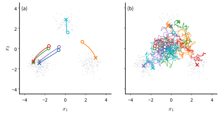
Two stochastic samplers must be kept apart. The ancestral chain of Section 17.2 adds the variance of the forward step, \(\sigma_t^2 - (\alpha_t / \alpha_s)^2 \sigma_s^2\), while \(\eta = 1\) adds the posterior variance, smaller by the factor \(\sigma_s^2 / \sigma_t^2\). On a thousand-step grid the factor is close to one and the two nearly agree; on fifty steps the ancestral sampler adds more noise than the posterior allows.
17.4.2 Fewer Steps
We isolate the error of a stride on the mixture, then turn to second-order solvers and step grids, and measure quality against the number of evaluations on images.
17.4.2.1 Skipping Steps on the Running Example
With the exact predictor, any difference between a ten-step sample and a thousand-step sample from the same start is error of the stride. The cell runs DDIM on the variance-preserving grid with 5 to 1,000 steps and prints the mean distance to the thousand-step samples and the spread (the mean squared distance to the nearest mode).
samples = {n: d2l.ddim_sample(pred_exact, z, vp, n)
           for n in (5, 10, 20, 50, 200, 1000)}
for n, x in samples.items():
    gap = (x - samples[1000]).norm(dim=1).mean()
    print(f'{n:4d} steps: distance to 1,000 steps {gap:.3f}, '
          f'spread {mix.summary(x)["spread"]:.3f}')
d2l.scatter_panels([samples[10][:2000], samples[200][:2000]],
                   ['10 steps', '200 steps'], data=mix.sample(2000));
5 steps: distance to 1,000 steps 0.411, spread 0.309
10 steps: distance to 1,000 steps 0.210, spread 0.380
20 steps: distance to 1,000 steps 0.107, spread 0.420
50 steps: distance to 1,000 steps 0.043, spread 0.451
200 steps: distance to 1,000 steps 0.009, spread 0.469
1000 steps: distance to 1,000 steps 0.000, spread 0.474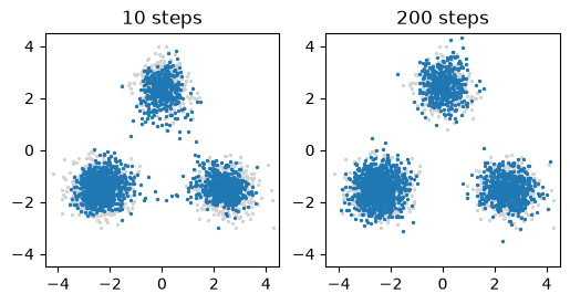
samples = {n: d2l.ddim_sample(pred_exact, z, vp, n)
           for n in (5, 10, 20, 50, 200, 1000)}
for n, x in samples.items():
    gap = jnp.linalg.norm(x - samples[1000], axis=1).mean()
    print(f'{n:4d} steps: distance to 1,000 steps {gap:.3f}, '
          f'spread {mix.summary(x)["spread"]:.3f}')
d2l.scatter_panels([samples[10][:2000], samples[200][:2000]],
                   ['10 steps', '200 steps'],
                   data=mix.sample(jax.random.key(1), 2000));
5 steps: distance to 1,000 steps 0.415, spread 0.309
10 steps: distance to 1,000 steps 0.213, spread 0.381
20 steps: distance to 1,000 steps 0.109, spread 0.422
50 steps: distance to 1,000 steps 0.043, spread 0.452
200 steps: distance to 1,000 steps 0.009, spread 0.469
1000 steps: distance to 1,000 steps 0.000, spread 0.474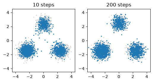
The distance halves each time the number of steps doubles, as for a first-order method: about 0.4 at five steps, 0.2 at ten and 0.04 at fifty, on a scale where the modes are five units apart. The error has a direction: the spread falls from about 0.47 at a thousand steps to 0.38 at ten, and the clouds in the left panel are visibly tighter than the data behind them. A stride holds the noise estimate at its value at the start, which for Gaussian data always removes too much noise (exercise 3), and the modes of the mixture behave like Gaussians. Since the spread rewards contraction, and a stochastic sample has no thousand-step counterpart, we compare \(\eta = 0\) with \(\eta = 1\) on images instead.
17.4.2.2 Second Order and the Step Grid
Euler’s method holds the slope fixed across a step, so its error over the whole run falls only in proportion to the step size. Heun’s method (Section 43.1.3) takes the Euler step as a trial, evaluates the slope again at the trial point, and moves with the average of the two slopes:
\[\bar{\mathbf{x}}' = \bar{\mathbf{x}}_t + (\bar\sigma_s - \bar\sigma_t)\, \hat{\boldsymbol\epsilon}(\bar{\mathbf{x}}_t, \bar\sigma_t), \qquad \bar{\mathbf{x}}_s = \bar{\mathbf{x}}_t + (\bar\sigma_s - \bar\sigma_t)\, \frac{\hat{\boldsymbol\epsilon}(\bar{\mathbf{x}}_t, \bar\sigma_t) + \hat{\boldsymbol\epsilon}(\bar{\mathbf{x}}', \bar\sigma_s)}{2}. \tag{17.4.6}\]
Its error falls with the square of the step size, at two evaluations per step. For standard Gaussian data the noise estimate is \(\hat{\boldsymbol\epsilon} = \bar\sigma \bar{\mathbf{x}} / (1 +
\bar\sigma^2)\), and the exact flow multiplies \(\bar{\mathbf{x}}\) by \(\sqrt{(1 + \bar\sigma_s^2) / (1 + \bar\sigma_t^2)}\). From \(\bar\sigma_t =
1\) to \(\bar\sigma_s = 0.5\) the exact factor is \(0.791\), Euler’s step gives \(0.75\) and Heun’s \(0.80\): errors of \(0.041\) and \(0.009\), a fifth of the error for twice the cost. The last step, to \(\bar\sigma = 0\), is an Euler step, and so is a first step from \(\bar\sigma = \infty\), so heun_sample spends \(2n - 1\) evaluations on \(n\) steps, or \(2n - 2\) from pure noise on the linear path.
Whether the second evaluation pays depends on where the steps are, and the answer depends on the field. On the exact field of a one-dimensional mixture (Section 43.6.4), Heun’s method loses to Euler’s below about forty evaluations when the steps are equal in \(t\), and wins at every budget from ten evaluations when the steps are crowded toward the data: step errors of opposite sign cancel, Euler’s on equal steps and Heun’s on crowded ones. Karras et al. (2022) crowd the steps by spacing \(\bar\sigma^{1/\rho}\) evenly,
\[\bar\sigma_i = \Big(\bar\sigma_{\max}^{1/\rho} + \tfrac{i}{n - 1}\big(\bar\sigma_{\min}^{1/\rho} - \bar\sigma_{\max}^{1/\rho}\big)\Big)^{\rho}, \qquad i = 0, \ldots, n - 1, \tag{17.4.7}\]
followed by a last step to \(\bar\sigma = 0\), with \(\bar\sigma_{\max} = 80\), \(\bar\sigma_{\min} = 0.002\) and \(\rho = 7\) for images in \([-1, 1]\); this is edm_grid. The grid is a choice of the sampler, separate from the training path, since make_pred translates any level to the network’s own time. The cell saves edm_grid and heun_sample, and prints \(\bar\sigma\) on this grid and on the ten-step grids of the variance-preserving and linear paths, even in time.
def edm_grid(steps, sigma_max=80.0, sigma_min=0.002, rho=7):
    """Karras et al.'s levels sigma_bar: even in sigma_bar^(1/rho), then 0."""
    hi, lo = sigma_max ** (1 / rho), sigma_min ** (1 / rho)
    return [(hi + i / (steps - 1) * (lo - hi)) ** rho
            for i in range(steps)] + [0.0]

@torch.no_grad()
def heun_sample(pred, x, sigma_bars):
    """Heun on d x_bar / d sigma_bar = eps: an Euler trial, then the average
    of the two slopes; from x at the first level to data, as ode_sample."""
    r0 = sigma_bars[0]
    xb = x if math.isinf(r0) else x * math.sqrt(1 + r0 ** 2)  # x / alpha
    for r_t, r_s in zip(sigma_bars[:-1], sigma_bars[1:]):
        x0, eps = d2l.pred_bar(pred, xb, r_t)
        x_next = x0 + r_s * eps                       # the Euler step
        if r_s > 0 and not math.isinf(r_t):           # no slope at 0 or inf
            x_next = xb + (r_s - r_t) * (
                eps + d2l.pred_bar(pred, x_next, r_s)[1]) / 2
        xb = x_next
    return xb

for name, levels in (('VP', vp.sigma_bars(10)), ('linear', lin.sigma_bars(10)),
                     ('EDM', d2l.edm_grid(10))):
    print(f'{name:7s}', ' '.join(f'{r:7.3g}' for r in levels))
VP 152 58.8 25.1 11.8 6.1 3.41 2.03 1.23 0.72 0.34 0
linear inf 9 4 2.33 1.5 1 0.667 0.429 0.25 0.111 0
EDM 80 42.4 21.1 9.72 4.07 1.5 0.47 0.117 0.0204 0.002 0def edm_grid(steps, sigma_max=80.0, sigma_min=0.002, rho=7):
"""Karras et al.'s levels sigma_bar: even in sigma_bar^(1/rho), then 0."""
hi, lo = sigma_max ** (1 / rho), sigma_min ** (1 / rho)
return [(hi + i / (steps - 1) * (lo - hi)) ** rho
for i in range(steps)] + [0.0]
def heun_sample(pred, x, sigma_bars):
"""Heun on d x_bar / d sigma_bar = eps: an Euler trial, then the average
of the two slopes; from x at the first level to data, as ode_sample."""
with jax.ensure_compile_time_eval(): # the grid is a constant
r = jnp.asarray(sigma_bars)
from_inf = bool(jnp.isinf(r[0]))
def step(xb, r):
r_t, r_s = r
x0, eps = d2l.pred_bar(pred, xb, r_t)
x_next = x0 + r_s * eps # the Euler step
correct = lambda _: xb + (r_s - r_t) * (
eps + d2l.pred_bar(pred, x_next, r_s)[1]) / 2
heun = jnp.isfinite(r_t) & (r_s > 0) # no slope at inf or 0
return jax.lax.cond(heun, correct, lambda _: x_next, None), None
xb = x if from_inf else x * jnp.sqrt(1 + r[0] ** 2) # x / alpha
return jax.lax.scan(step, xb, (r[:-1], r[1:]))[0]
for name, levels in (('VP', vp.sigma_bars(10)), ('linear', lin.sigma_bars(10)),
('EDM', d2l.edm_grid(10))):
print(f'{name:7s}', ' '.join(f'{float(r):7.3g}' for r in levels))VP 152 58.8 25.1 11.8 6.1 3.41 2.03 1.23 0.72 0.34 0
linear inf 9 4 2.33 1.5 1 0.667 0.429 0.25 0.111 0
EDM 80 42.4 21.1 9.72 4.07 1.5 0.47 0.117 0.0204 0.002 0The variance-preserving grid spends four of its ten steps above \(\bar\sigma = 6\), where all noisy points look alike, and reaches the data from \(0.34\). The linear grid’s finite levels run from \(9\) to \(0.11\). The EDM grid starts at \(80\) but crowds its last levels down to \(0.002\). Exponential integrators such as DPM-Solver (Lu et al. 2022) take steps in \(\log \bar\sigma\) (exercise 6).
17.4.2.3 Quality against Evaluations on Images
On images the field is learned. We train the unconditional version of the model of Section 17.3, the U-Net of about 1.2 million parameters without its label input, on the velocity of the linear path for ten thousand updates, a few minutes on one GPU, and sample from the moving average of its weights.
X, y, X_test, y_test = d2l.load_fashion_mnist_pm1()

def batch_fn():
    return X[torch.randint(0, len(X), (128,), device=X.device)]

torch.manual_seed(0)
net = d2l.UNet(ch=64).to(X.device)
net, ema, _ = d2l.train_regression(net, d2l.regression_loss(lin, 'velocity'),
                                   batch_fn, 10_000)
pred = d2l.make_pred(ema, lin, 'velocity')
X, y, X_test, y_test = d2l.load_fashion_mnist_pm1()
def batch_fn(key):
return X[jax.random.randint(key, (128,), 0, len(X))]
net = d2l.UNet(ch=64, rngs=nnx.Rngs(0))
net, ema, _ = d2l.train_regression(net, d2l.regression_loss(lin, 'velocity'),
batch_fn, 10_000, jax.random.key(0))
pred = d2l.make_pred(ema, lin, 'velocity')We score samples by the Fréchet distance (FD) of Section 17.3 in d2l.FeatureCNN features, 1,000 generated against 1,000 test images, read against the floor of two disjoint sets of 1,000 real images.
cnn = d2l.fashion_feature_cnn(X, y)
features = lambda imgs: d2l.fd_features(cnn, imgs)
f_test = features(X_test[:1000])
floor = d2l.fid_score(features(X_test[1000:2000]), f_test)
print(f'floor, 1,000 real images against 1,000 others: FD {floor:.2f}')
floor, 1,000 real images against 1,000 others: FD 0.82cnn = d2l.fashion_feature_cnn(X, y)
features = lambda imgs: d2l.fd_features(cnn, imgs)
f_test = features(X_test[:1000])
floor = d2l.fid_score(features(X_test[1000:2000]), f_test)
print(f'floor, 1,000 real images against 1,000 others: FD {floor:.2f}')floor, 1,000 real images against 1,000 others: FD 0.84Each sampler draws 1,000 images from the same noise. “VP” and “linear” denote even steps in time on that path, so DDIM with \(\eta = 0\) on “VP” is Euler’s method on the first grid printed above; “EDM” denotes the crowded grid. We count network evaluations, not steps.
families = {  # name: (sampler(pred, noise, n), step counts n)
    'ancestral, VP': (lambda p, z, n: d2l.ancestral_sample(p, z, vp, n),
                      (50, 200, 1000)),
    'DDIM eta=1, VP': (lambda p, z, n: d2l.ddim_sample(p, z, vp, n, 1.0),
                       (10, 20, 50, 100)),
    'DDIM eta=0, VP': (lambda p, z, n: d2l.ddim_sample(p, z, vp, n),
                       (10, 20, 50, 100)),
    'Euler, linear': (lambda p, z, n: d2l.ode_sample(p, z, lin.sigma_bars(n)),
                      (10, 20, 50)),
    'Euler, EDM': (lambda p, z, n: d2l.ode_sample(p, z, d2l.edm_grid(n)),
                   (10, 20, 50)),
    'Heun, linear': (lambda p, z, n: d2l.heun_sample(p, z, lin.sigma_bars(n)),
                     (5, 10, 25)),
    'Heun, EDM': (lambda p, z, n: d2l.heun_sample(p, z, d2l.edm_grid(n)),
                  (5, 10, 25))}

def evaluations(name, n):  # Heun's second slope is skipped at inf and at 0
    return {'Heun, linear': 2 * n - 2, 'Heun, EDM': 2 * n - 1}.get(name, n)

torch.manual_seed(1)
noise = torch.randn(1000, 1, 28, 28, device=X.device)
images = {name: [f(pred, noise, n).clamp(-1, 1) for n in steps]
          for name, (f, steps) in families.items()}
fd = {name: [d2l.fid_score(features(x), f_test) for x in xs]
      for name, xs in images.items()}
for name, (_, steps) in families.items():
    print(f'{name:15s}', '  '.join(f'{evaluations(name, n):4d}: {v:5.2f}'
                                   for n, v in zip(steps, fd[name])))
ancestral, VP 50: 11.86 200: 3.24 1000: 2.25
DDIM eta=1, VP 10: 14.34 20: 6.89 50: 3.89 100: 2.95
DDIM eta=0, VP 10: 9.07 20: 4.59 50: 2.76 100: 2.35
Euler, linear 10: 6.90 20: 3.60 50: 2.52
Euler, EDM 10: 13.13 20: 5.77 50: 3.28
Heun, linear 8: 7.13 18: 2.07 48: 1.93
Heun, EDM 9: 11.69 19: 2.16 49: 2.13families = { # name: (sampler(pred, noise, n, key), step counts n)
'ancestral, VP': (lambda p, z, n, k: d2l.ancestral_sample(p, z, vp, n, k),
(50, 200, 1000)),
'DDIM eta=1, VP': (lambda p, z, n, k: d2l.ddim_sample(p, z, vp, n, 1.0, k),
(10, 20, 50, 100)),
'DDIM eta=0, VP': (lambda p, z, n, k: d2l.ddim_sample(p, z, vp, n),
(10, 20, 50, 100)),
'Euler, linear': (lambda p, z, n, k: d2l.ode_sample(p, z,
lin.sigma_bars(n)),
(10, 20, 50)),
'Euler, EDM': (lambda p, z, n, k: d2l.ode_sample(p, z, d2l.edm_grid(n)),
(10, 20, 50)),
'Heun, linear': (lambda p, z, n, k: d2l.heun_sample(p, z,
lin.sigma_bars(n)),
(5, 10, 25)),
'Heun, EDM': (lambda p, z, n, k: d2l.heun_sample(p, z, d2l.edm_grid(n)),
(5, 10, 25))}
def evaluations(name, n): # Heun's second slope is skipped at inf and at 0
return {'Heun, linear': 2 * n - 2, 'Heun, EDM': 2 * n - 1}.get(name, n)
k_noise, k_run = jax.random.split(jax.random.key(1))
noise = jax.random.normal(k_noise, (1000, 28, 28, 1))
keys = iter(jax.random.split(k_run, 32))
images = {name: [f(pred, noise, n, next(keys)).clip(-1, 1) for n in steps]
for name, (f, steps) in families.items()}
fd = {name: [d2l.fid_score(features(x), f_test) for x in xs]
for name, xs in images.items()}
for name, (_, steps) in families.items():
print(f'{name:15s}', ' '.join(f'{evaluations(name, n):4d}: {v:5.2f}'
for n, v in zip(steps, fd[name])))ancestral, VP 50: 14.76 200: 3.08 1000: 1.87
DDIM eta=1, VP 10: 14.70 20: 6.79 50: 4.60 100: 3.21
DDIM eta=0, VP 10: 9.62 20: 5.02 50: 3.03 100: 2.55
Euler, linear 10: 7.08 20: 3.91 50: 2.78
Euler, EDM 10: 13.02 20: 6.07 50: 3.53
Heun, linear 8: 7.60 18: 2.38 48: 2.06
Heun, EDM 9: 13.36 19: 2.32 49: 2.29The plot shows each FD against the number of evaluations.
evals = [[evaluations(name, n) for n in steps]
         for name, (_, steps) in families.items()]
d2l.plot(evals + [[5, 1000]], list(fd.values()) + [[floor, floor]],
         'network evaluations', 'FD', legend=list(families) + ['floor'],
         xscale='log', yscale='log', figsize=(6, 4),
         fmts=('o-', 's-', '^-', 'v--', 'D--', 'x-.', '+-.', 'k:'))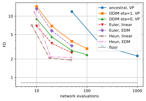
evals = [[evaluations(name, n) for n in steps]
         for name, (_, steps) in families.items()]
d2l.plot(evals + [[5, 1000]], list(fd.values()) + [[floor, floor]],
         'network evaluations', 'FD', legend=list(families) + ['floor'],
         xscale='log', yscale='log', figsize=(6, 4),
         fmts=('o-', 's-', '^-', 'v--', 'D--', 'x-.', '+-.', 'k:'))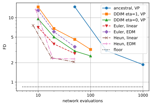
The thousand-step ancestral chain, the reference, scores two to three times the floor. Deterministic DDIM at fifty steps scores about 3, within about 1.5 times the chain’s FD at a twentieth of the evaluations, which reproduces the central result of J. Song et al. (2021) . At equal numbers of steps, \(\eta = 0\) beats \(\eta = 1\) by about a third at 10, 20 and 50 steps, and the gap narrows to about a fifth at a hundred, as the trade-off above predicts. The ancestral sampler at fifty steps scores worse than deterministic DDIM at ten, because it adds more noise than the posterior allows; its images are speckled (exercise 7).
Heun’s method on the crowded grid scores about 2 at nineteen evaluations, better than DDIM at fifty; on the linear grid at forty-eight evaluations it scores about 2, the quality of the thousand-step chain at a twentieth of its evaluations. The grid matters as much as the method: with ten steps, Euler’s method scores about 7 on the linear grid, 9 to 10 on the variance-preserving grid (where it is DDIM), and about 13 on the crowded grid. Crowding the steps toward the data hurts Euler’s method at every budget, and Heun’s at eight and at forty-eight evaluations; only near twenty do the two grids tie. On this model the even grid of the linear path serves both methods best.
The one-dimensional result does not transfer, and the printed grids suggest why. With ten levels the crowded grid spends four steps above \(\bar\sigma = 4\), where all noisy images look alike, and three below \(0.12\), where a \(28 \times 28\) garment barely changes, leaving three steps for the range in which its shape is decided; the linear grid spends seven of its ten steps there. Karras et al. (2022) tuned \(\rho = 7\) for 35 to 79 evaluations on larger images.
Below are eight images from each of four samplers, all from the same eight noise images: the ancestral chain with 1,000 steps, DDIM with 10 and with 50 steps, and Heun’s method on the crowded grid with 19 evaluations.
rows = [images['ancestral, VP'][2], images['DDIM eta=0, VP'][0],
        images['DDIM eta=0, VP'][2], images['Heun, EDM'][1]]
d2l.show_gray(torch.cat([x[:8] for x in rows]), 4, 8);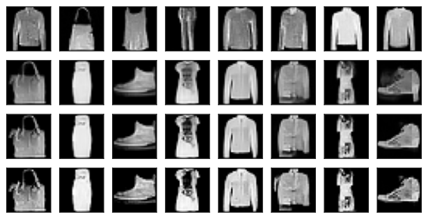
rows = [images['ancestral, VP'][2], images['DDIM eta=0, VP'][0],
        images['DDIM eta=0, VP'][2], images['Heun, EDM'][1]]
d2l.show_gray(jnp.concatenate([x[:8] for x in rows]), 4, 8);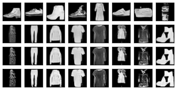
The last three rows match column by column: the deterministic samplers approximate one map from noise to images, and ten steps slightly blur the image that fifty steps and Heun’s method agree on. The first row does not match, because the ancestral chain’s image depends as much on the noise it adds as on its start.
17.4.3 Inversion and Editing
A deterministic sampler integrates a differential equation, which can be run in either direction. Running it backwards assigns each image a noise image, its code, which gives interpolation, editing and inpainting without retraining.
17.4.3.1 The Latent Code
ddim_invert runs the deterministic sampler backwards, from an image at \(t = 0\) toward noise. Each step evaluates the network at the current point but tells it the noise level of the step’s upper end, since the predictor needs \(\sigma > 0\) and the first point has none.
@torch.no_grad()
def ddim_invert(pred, x, path, steps, t_end=1.0):
    """Deterministic DDIM run backwards, from data x at t = 0 to t_end."""
    a, s = path.grid(steps, 0.0, t_end)
    for i in range(steps):
        eps = pred(x, a[i + 1], s[i + 1])[1]    # x read at the next level
        x = a[i + 1] * (x - s[i] * eps) / a[i] + s[i + 1] * eps
    return x
def ddim_invert(pred, x, path, steps, t_end=1.0):
"""Deterministic DDIM run backwards, from data x at t = 0 to t_end."""
a, s = path.grid(steps, 0.0, t_end)
def step(x, inputs):
a_t, s_t, a_s, s_s = inputs
eps = pred(x, a_s, s_s)[1] # x read at the next level
return a_s * (x - s_t * eps) / a_t + s_s * eps, None
return jax.lax.scan(step, x, (a[:-1], s[:-1], a[1:], s[1:]))[0]In the coordinates \((\bar{\mathbf{x}}, \bar\sigma)\) each inverse step is the Euler step \(\bar{\mathbf{x}}_{t'} = \bar{\mathbf{x}}_t + (\bar\sigma_{t'} - \bar\sigma_t)\, \hat{\boldsymbol\epsilon}\) taken upward, from the level \(t\) to the next level \(t' > t\). The decoder evaluates the noise estimate at the upper point, the encoder at the lower one, the only point it has; the two differ by the change of \(\hat{\boldsymbol\epsilon}\) over one step, so the round trip is inexact even with an exact predictor. The cell encodes and decodes 100 test images with 10 to 100 steps on the linear path.
x0 = X_test[:100]
codes = {n: d2l.ddim_invert(pred, x0, lin, n) for n in (10, 20, 50, 100)}
recon = {n: d2l.ddim_sample(pred, code, lin, n) for n, code in codes.items()}
for n in codes:
    print(f'{n:3d} steps: squared error per pixel '
          f'{((recon[n] - x0) ** 2).mean():.4f}, code std {codes[n].std():.2f}')
d2l.show_gray(torch.cat([x0[:8], recon[10][:8], recon[50][:8]]), 3, 8);
10 steps: squared error per pixel 0.0603, code std 0.55
20 steps: squared error per pixel 0.0380, code std 0.61
50 steps: squared error per pixel 0.0174, code std 0.72
100 steps: squared error per pixel 0.0101, code std 0.80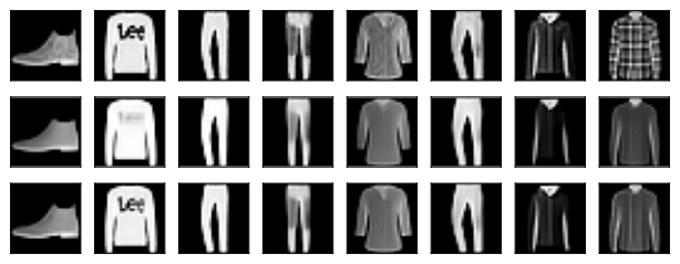
x0 = X_test[:100]
codes = {n: d2l.ddim_invert(pred, x0, lin, n) for n in (10, 20, 50, 100)}
recon = {n: d2l.ddim_sample(pred, code, lin, n) for n, code in codes.items()}
for n in codes:
    print(f'{n:3d} steps: squared error per pixel '
          f'{((recon[n] - x0) ** 2).mean():.4f}, code std {codes[n].std():.2f}')
d2l.show_gray(jnp.concatenate([x0[:8], recon[10][:8], recon[50][:8]]), 3, 8);
10 steps: squared error per pixel 0.0659, code std 0.54
20 steps: squared error per pixel 0.0399, code std 0.60
50 steps: squared error per pixel 0.0174, code std 0.73
100 steps: squared error per pixel 0.0098, code std 0.82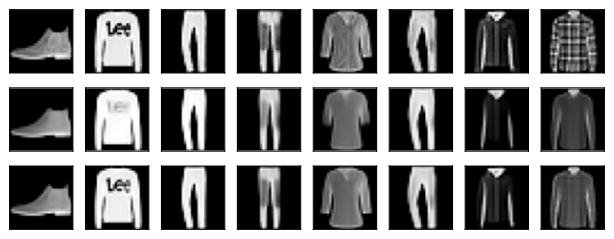
The reconstruction error falls with the number of steps, more slowly than the step size, since the learned field adds errors of its own: at fifty steps (third row) the reconstructions are close to the originals, at ten (second row) they lose fine detail. The codes are not typical noise: their standard deviation lies below one, approaching one only as the steps get shorter.
Because the sampler is a continuous function of its code, we can move between two images by interpolating between their codes. A straight line is the wrong path: the average of two independent noise images has a norm smaller by about \(\sqrt{2}\), which noise images of this dimension almost never have. Spherical interpolation moves along the great circle between the two codes instead,
\[\mathbf{z}_u = \frac{\sin\big((1 - u)\omega\big)\, \mathbf{z}_0 + \sin(u \omega)\, \mathbf{z}_1}{\sin \omega}, \qquad \cos \omega = \frac{\mathbf{z}_0^\top \mathbf{z}_1}{\|\mathbf{z}_0\| \|\mathbf{z}_1\|}, \tag{17.4.8}\]
which keeps the norm close to that of the endpoints. We decode eight points between the 50-step codes of the first two test images.
z0, z1 = codes[50][0], codes[50][1]
omega = torch.arccos(((z0 * z1).sum() / (z0.norm() * z1.norm())).clamp(-1, 1))
u = torch.linspace(0, 1, 8, device=z0.device).reshape(-1, 1, 1, 1)
zs = (torch.sin((1 - u) * omega) * z0 + torch.sin(u * omega) * z1
      ) / torch.sin(omega)
d2l.show_gray(d2l.ddim_sample(pred, zs, lin, 50), 1, 8);
z0, z1 = codes[50][0], codes[50][1]
omega = jnp.arccos(jnp.clip(
    (z0 * z1).sum() / (jnp.linalg.norm(z0) * jnp.linalg.norm(z1)), -1, 1))
u = jnp.linspace(0, 1, 8).reshape(-1, 1, 1, 1)
zs = (jnp.sin((1 - u) * omega) * z0 + jnp.sin(u * omega) * z1
      ) / jnp.sin(omega)
d2l.show_gray(d2l.ddim_sample(pred, zs, lin, 50), 1, 8);
The row moves from a reconstruction of the first test image to one of the second, and every intermediate code decodes to a plausible item.
17.4.3.2 Editing by Partial Noising
Inversion runs an image all the way to noise; stopping part of the way gives an editor. Meng et al. (2022) noise a rough input, such as a sketch or a crude collage, to an intermediate time \(t_0\) with \(\mathbf{x}_{t_0} = \alpha_{t_0} \mathbf{y} + \sigma_{t_0} \boldsymbol\epsilon\), and run the sampler from \(t_0\) back to the data. The noise hides the details of the input that real images do not have, the sampler replaces them by details that real images do have, and the coarse layout survives. The time \(t_0\) sets the balance between fidelity to the input and realism.
Our rough inputs are the ten class-mean images, blurred silhouettes that no real garment looks like, each noised a hundred times to \(t_0 \in \{0.3, 0.5, 0.7, 1\}\) and integrated back with 25 DDIM steps. The cell prints the squared distance per pixel to the input (fidelity) and the FD of the 1,000 outputs (realism); the row \(t_0 = 0\) holds the inputs.
means = torch.stack([X[y == c].mean(0) for c in range(10)])
inputs = means.repeat(100, 1, 1, 1)                  # 1,000 inputs
torch.manual_seed(2)
eps = torch.randn_like(inputs)
edits = {0.0: inputs}
for t0 in (0.3, 0.5, 0.7, 1.0):
    x_t0 = lin.sample(inputs, torch.full((1000,), t0, device=X.device), eps)
    edits[t0] = d2l.ddim_sample(pred, x_t0, lin, 25, t_start=t0).clamp(-1, 1)
for t0, x in edits.items():
    print(f't0 = {t0:.1f}: squared distance to the input '
          f'{((x - inputs) ** 2).mean():.3f}, '
          f'FD {d2l.fid_score(features(x), f_test):.2f}')
d2l.show_gray(torch.cat([x[:10] for x in edits.values()]), 5, 10);
t0 = 0.0: squared distance to the input 0.000, FD 92.29
t0 = 0.3: squared distance to the input 0.019, FD 33.37
t0 = 0.5: squared distance to the input 0.046, FD 13.58
t0 = 0.7: squared distance to the input 0.091, FD 5.38
t0 = 1.0: squared distance to the input 0.435, FD 3.22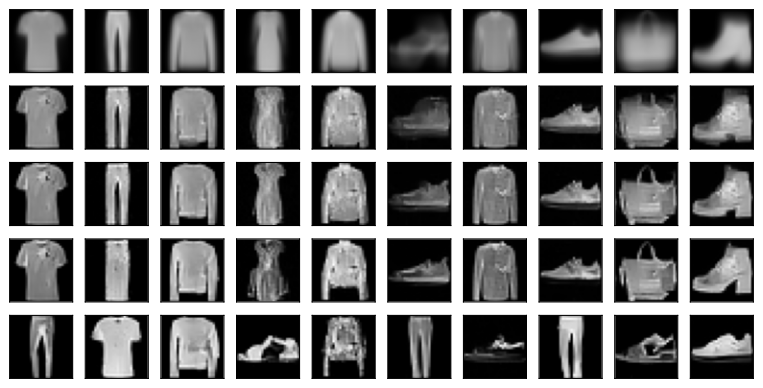
means = jnp.stack([X[y == c].mean(0) for c in range(10)])
inputs = jnp.tile(means, (100, 1, 1, 1))             # 1,000 inputs
eps = jax.random.normal(jax.random.key(2), inputs.shape)
edits = {0.0: inputs}
for t0 in (0.3, 0.5, 0.7, 1.0):
    x_t0 = lin.sample(inputs, jnp.full((1000,), t0), eps)
    edits[t0] = d2l.ddim_sample(pred, x_t0, lin, 25, t_start=t0).clip(-1, 1)
for t0, x in edits.items():
    print(f't0 = {t0:.1f}: squared distance to the input '
          f'{((x - inputs) ** 2).mean():.3f}, '
          f'FD {d2l.fid_score(features(x), f_test):.2f}')
d2l.show_gray(jnp.concatenate([x[:10] for x in edits.values()]), 5, 10);
t0 = 0.0: squared distance to the input 0.000, FD 87.91
t0 = 0.3: squared distance to the input 0.018, FD 30.24
t0 = 0.5: squared distance to the input 0.046, FD 12.11
t0 = 0.7: squared distance to the input 0.092, FD 4.70
t0 = 1.0: squared distance to the input 0.449, FD 3.01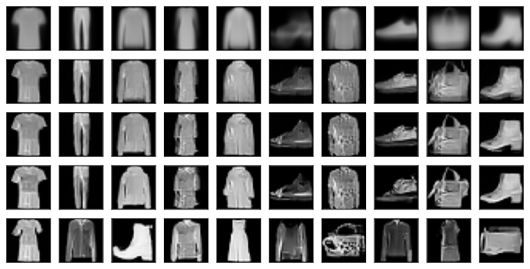
The distance to the input grows with \(t_0\), and the FD falls from far above that of any sampler toward that of fresh samples. At \(t_0 = 0.3\) each output keeps the silhouette of its mean image and gains the seams, prints and edges of a real garment; at \(0.5\) and \(0.7\) class and pose survive while the details vary; at \(t_0 = 1\) the output is an unrelated sample.
17.4.3.3 Inpainting and Posterior Sampling
Suppose that we know part of an image, the upper half, say, and want the model to fill in the rest. Write \(\mathbf{m}\) for the mask that is one on the known pixels and \(\mathbf{y}\) for their values. At every level we know what the known pixels of \(\mathbf{x}_s\) should look like, \(\alpha_s \mathbf{y}\) plus noise of scale \(\sigma_s\), so replacement inpainting (Y. Song et al. 2021; Lugmayr et al. 2022) takes each sampler step as usual and then overwrites the known pixels with a fresh noisy copy of \(\mathbf{y}\) at the new level,
\[\mathbf{x}_s \leftarrow \mathbf{m} \odot \big(\alpha_s \mathbf{y} + \sigma_s \boldsymbol\xi\big) + (\mathbf{1} - \mathbf{m}) \odot \mathbf{x}_s. \tag{17.4.9}\]
inpaint therefore runs the sampler one step at a time.
@torch.no_grad()
def inpaint(pred, known, mask, path, steps):
    """DDIM from noise that resets the known pixels (mask 1) at each level."""
    a, s = path.grid(steps)
    x = torch.randn_like(known)
    for i in range(steps):
        x0, eps = pred(x, a[i], s[i])
        x = a[i + 1] * x0 + s[i + 1] * eps            # one DDIM step, eta = 0
        noised = a[i + 1] * known + s[i + 1] * torch.randn_like(x)
        x = mask * noised + (1 - mask) * x            # keep the known pixels
    return x
def inpaint(pred, known, mask, path, steps, key):
"""DDIM from noise that resets the known pixels (mask 1) at each level."""
a, s = path.grid(steps)
def step(x, inputs):
a_t, s_t, a_s, s_s, key = inputs
x0, eps = pred(x, a_t, s_t)
x = a_s * x0 + s_s * eps # one DDIM step, eta = 0
noised = a_s * known + s_s * jax.random.normal(key, x.shape)
return mask * noised + (1 - mask) * x, None # keep the known pixels
keys = jax.random.split(key, steps + 1)
x = jax.random.normal(keys[0], known.shape)
return jax.lax.scan(step, x, (a[:-1], s[:-1], a[1:], s[1:], keys[1:]))[0]We keep the upper half of eight test images and ask for three completions of each, from different noise. The rows show the known halves, the three completions and the originals.
mask = torch.zeros(1, 1, 28, 28, device=X.device)
mask[..., :14, :] = 1                                # the upper half is known
torch.manual_seed(3)
fills = inpaint(pred, X_test[:8].repeat(3, 1, 1, 1), mask, lin, 50)
d2l.show_gray(torch.cat([X_test[:8] * mask, fills, X_test[:8]]), 5, 8);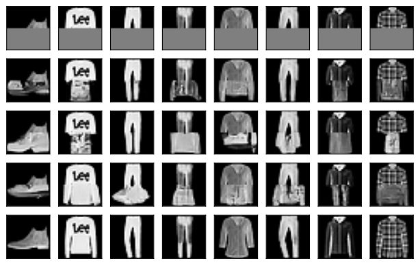
mask = jnp.zeros((1, 28, 28, 1)).at[:, :14].set(1)  # the upper half is known
fills = inpaint(pred, jnp.tile(X_test[:8], (3, 1, 1, 1)), mask, lin, 50,
                jax.random.key(3))
d2l.show_gray(jnp.concatenate([X_test[:8] * mask, fills, X_test[:8]]), 5, 8);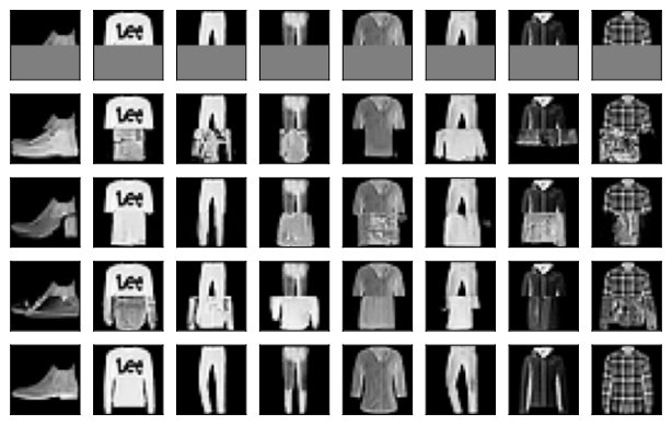
Most completions continue the known half into a plausible garment of the same kind, some are malformed, and the three completions of one image differ. The boundary is not always clean: the network sees the known pixels only through noisy copies, and the halves can disagree along the seam (exercise 9 measures and repairs this).
Most measurements, such as a blurred or low-resolution copy, are not a subset of the pixels; for these, Bayes’ rule adds the gradient of the measurement’s log-likelihood to the score, as guidance did for a class label in Section 17.3, and Chung et al. (2023) evaluate that likelihood at the network’s estimate \(\hat{\mathbf{x}}_0(\mathbf{x}_t)\).
17.4.4 Summary
Training fixes only the distribution of the noisy point at each time, so one network serves a family of samplers, from DDIM, which is Euler’s method for the probability-flow ODE in the coordinates \((\mathbf{x}/\alpha, \sigma/\alpha)\), to a stochastic sampler with the posterior variance. Fresh noise corrects errors but needs short steps, so the deterministic sampler wins at small budgets: on Fashion-MNIST fifty DDIM steps came within about 1.5 times the FD of the thousand-step chain, and Heun’s method matched the chain at about fifty evaluations, with the grid mattering as much as the method. Run backwards, the deterministic sampler gives every image a code, and with it interpolation, editing and inpainting.
We have trained every model so far by an unweighted squared error on a target we picked, without asking why this loss is the right one or how the choices of target, path and weighting compare. Section 17.5 derives the loss from the likelihood and measures the choices.
17.4.5 Exercises
- Admissible noise scales. The family Equation 17.4.2 needs \(\tilde\sigma \leq \sigma_s\).
- Show that a strength \(\eta\) is admissible on a step from \(t\) to \(s\) exactly when \(\eta^2 \leq 1 / (1 - \kappa^2)\), so that \(\eta = 1\) is admissible on every grid. At the largest admissible \(\eta\), what does the step keep of \(\mathbf{x}_t\) beyond \(\hat{\mathbf{x}}_0\)?
- Show that the last step of
ddim_sample, to \(t = 0\), returns \(\hat{\mathbf{x}}_0\) for every \(\eta\). - Evaluate the fraction \(f\) of fresh noise at \(\eta = 1\) on every step of the variance-preserving grids with 10 and with 200 steps. What does the \(\eta = 1\) sampler carry from one level to the next on the ten-step grid?
- The forward step and the Markov member. ● Given \(\mathbf{x}_0\), draw \(\mathbf{x}_t = \alpha_t \mathbf{x}_0 + \sigma_t \boldsymbol\epsilon\) and \(\mathbf{x}_s\) from Equation 17.4.2 with the same \(\boldsymbol\epsilon\).
- Compute the mean and the covariance of \(\mathbf{x}_t\) given \(\mathbf{x}_s\) and \(\mathbf{x}_0\) by conditioning the joint Gaussian.
- Show that the mean depends on \(\mathbf{x}_0\) unless \(\tilde\sigma\) takes its value at \(\eta = 1\), and that the conditional is then the forward step \(\mathbf{x}_t = (\alpha_t / \alpha_s) \mathbf{x}_s + \sqrt{\sigma_t^2 - (\alpha_t / \alpha_s)^2 \sigma_s^2}\, \boldsymbol\nu\) of the noising chain of the previous section. Conclude that this chain is the only member of the family whose forward process is Markov.
- Show that with \(\tilde\sigma = 0\) at every step the forward process is \(\mathbf{x}_t = \alpha_t \mathbf{x}_0 + \sigma_t \boldsymbol\epsilon\) with one \(\boldsymbol\epsilon\) shared by all times. Why can the regression not tell these forward processes apart?
- Gaussian data. Let the data be one-dimensional with distribution \(\mathcal{N}(0, v)\), and work in the coordinates \((\bar x, \bar\sigma)\).
- Show that the exact noise estimate is \(\hat\epsilon = \bar\sigma \bar x / (v + \bar\sigma^2)\), that one deterministic stride from \(\bar\sigma\) to \(\bar\sigma'\) multiplies \(\bar x\) by \((v + \bar\sigma \bar\sigma') / (v + \bar\sigma^2)\), and that the exact flow multiplies it by \(\sqrt{(v + \bar\sigma'^2) / (v + \bar\sigma^2)}\).
- Show that the factor of the stride never exceeds the exact one, with equality only for \(\bar\sigma' = \bar\sigma\). What does this imply for the variance of deterministic samples of Gaussian data on any grid?
- Take \(v = 0.25\), the variance of one coordinate of a mode of
mix. Compute the standard deviation of deterministic samples from \(x_1 \sim \mathcal{N}(0, 1)\) on the variance-preserving grids with 200, 50, 20, 10 and 5 steps, and compare it with \(0.5\) and with the spreads printed in this section.
- [code] The strength \(\eta\) and the code. Use the image model of this section.
- Compute the FD of 1,000 samples of
ddim_samplefor \(\eta \in \{0, 0.25, 0.5, 1\}\) at 10, 20 and 50 steps. - Fix one noise image \(\mathbf{x}_1\) and draw 16 samples from it for each \(\eta\) with different random seeds. Compute the standard deviation of each pixel across the 16 samples and average it over the pixels. How much does the image depend on \(\mathbf{x}_1\) at each \(\eta\)?
- Which \(\eta\) would you use at each budget, and which if you need the sample to be a function of its code?
- Compute the FD of 1,000 samples of
- [code] Inversion on both examples. Encode 20,000 draws of
mixwithddim_invertandpred_exacton the variance-preserving grid with 10, 20, 50, 100 and 200 steps, and decode each set of codes withddim_sampleon the same grid.- How does the mean reconstruction error depend on the number of steps? Does it fall in proportion to the step size?
- Compute the mean and the covariance of the 200-step codes. Are they those of standard Gaussian noise?
- Repeat part (a) for the 100 test images with
predon the linear path, adding 200 steps, and compare the trend with Table 2 of J. Song et al. (2021) .
- [extended] A second-order sampler in log-SNR. ●● DPM-Solver-2 (Lu et al. 2022) takes a step from \(\bar\sigma\) to \(\bar\sigma'\) in two evaluations, the second at the midpoint \(\bar\sigma_m = \sqrt{\bar\sigma \bar\sigma'}\) in \(\log \bar\sigma\): \(\bar{\mathbf{x}}_m = \bar{\mathbf{x}} + (\bar\sigma_m - \bar\sigma)\,
\hat{\boldsymbol\epsilon}(\bar{\mathbf{x}}, \bar\sigma)\) and \(\bar{\mathbf{x}}' = \bar{\mathbf{x}} + (\bar\sigma' - \bar\sigma)\,
\hat{\boldsymbol\epsilon}(\bar{\mathbf{x}}_m, \bar\sigma_m)\).
- Let \(h = \log(\bar\sigma / \bar\sigma')\). Write the exact change of \(\bar{\mathbf{x}}\) over the step as an integral of \(\hat{\boldsymbol\epsilon}\) along the trajectory, and show that the local error of the update is \(O(\bar\sigma h^3)\) while that of the Euler step is \(O(\bar\sigma h^2)\). Assume that \(\hat{\boldsymbol\epsilon}\) is a smooth function of \(\log \bar\sigma\) along the trajectory and Lipschitz in \(\bar{\mathbf{x}}\).
- Implement the update with the interface
pred(x, alpha, sigma), using \(\alpha = 1 / \sqrt{1 + \bar\sigma^2}\) and \(\sigma = \bar\sigma \alpha\), and take the last step to \(\bar\sigma = 0\) with Euler’s method. Compare it withode_sampleandheun_sampleat about 11, 21 and 51 evaluations, on the mixture withpred_exactby the distance to a 1,000-step reference, and on images by the FD. - Repeat with levels evenly spaced in \(\log \bar\sigma\) between 80 and 0.002. Which combination of method and grid is best at each budget?
- [code] Fewer ancestral steps. Run
ancestral_sampleandddim_samplewith \(\eta = 1\) on the mixture withpred_exact, on the variance-preserving grids with 200, 50, 20 and 10 steps, from 20,000 starting points.- Compare the
mix.summarystatistics of the two samplers with those of the data. Where does each sampler break first: in the mode weights, in the spread or in the stray fraction? - Relate the change of the spread to the variance error of one ancestral step (exercise 4) and to the factor \(\sigma_s^2 / \sigma_t^2\) between the two samplers’ variances.
- Show 16 images of each sampler at 50 steps on the image model, and explain the speckle of the ancestral ones.
- Compare the
- The optimal reverse variance. ● A stochastic step from \(t\) to \(s\) moves to the posterior mean \(\alpha_s \hat{\mathbf{x}}_0 + \sigma_s \kappa
\hat{\boldsymbol\epsilon}\) and adds Gaussian noise of variance \(v\) per coordinate. Ho et al. (2020) tried the forward-step variance and the posterior variance; Bao et al. (2022) found the best \(v\) for any data. Assume exact estimates, and let \(\bar e_t =
\mathbb{E}\|\boldsymbol\epsilon - \hat{\boldsymbol\epsilon}\|^2 / d\) be the error per coordinate of the exact noise estimate at time \(t\) in \(d\) dimensions.
- Exercise 5a shows that the true reverse transition \(q(\mathbf{x}_s \mid \mathbf{x}_t)\) has covariance \(\tau^2 \mathbf{I} + c^2 \textrm{Cov}(\mathbf{x}_0 \mid \mathbf{x}_t)\), where \(c\) is the coefficient of \(\mathbf{x}_0\) in the mean of \(q(\mathbf{x}_s \mid \mathbf{x}_t, \mathbf{x}_0)\). Write that mean as \(\alpha_s \mathbf{x}_0 + \sigma_s \kappa \boldsymbol\epsilon\) with \(\boldsymbol\epsilon = (\mathbf{x}_t - \alpha_t \mathbf{x}_0)/\sigma_t\), and conclude that \(\tau^2 = \tilde\sigma^2\), the posterior variance, and \(c = k = \alpha_s - \sigma_s \kappa\, \alpha_t / \sigma_t\). What is the mean of the true reverse transition?
- Show that the \(v\) that minimizes the expected KL divergence from \(q(\mathbf{x}_s \mid \mathbf{x}_t)\) to the Gaussian step is \(v^\star = \tilde\sigma^2 + k^2 \bar\sigma_t^2 \bar e_t\), and that \(\bar e_t = 1 - \sigma_t^2\, \mathbb{E}\|\nabla \log p_t(\mathbf{x}_t)\|^2 / d\), so that \(v^\star\) follows from the score alone.
- Show that \(v^\star\) is the posterior variance when the data are one point, and the forward-step variance when the data are standard Gaussian on the variance-preserving path.
- (Optional, code.) Estimate \(\bar e_t\) on the mixture with
pred_exacton the 50-step variance-preserving grid, and compare the spread of 20,000 samples of the stochastic step with the three variances.
- [code] Inpainting with harmonization. ● The completions of
inpaintcan disagree with the known half along the boundary.- Measure the seam: the mean absolute difference between rows 13 and 14 of the completions, against the same quantity for real test images.
- RePaint (Lugmayr et al. 2022) lets the two halves exchange information: after each step from \(t\) to \(s\), it noises the result back to \(t\) with the forward step and repeats the step, \(r\) times per level. Implement it with \(r \in \{1, 5, 10\}\) at 50 levels and measure the seam again. What does each repetition cost?
- Draw five completions of one test image for each \(r\). How varied are they?
- [code] A rescaled schedule. ● Let \(c_t = 1 + t(1 - t)\) and define a path with \(\alpha'_t = c_t (1 - t)\) and \(\sigma'_t = c_t t\), which has the same endpoints as the linear path.
- Show that the two paths have the same log-SNR at every \(t\), and that the deterministic DDIM steps of Equation 17.4.3 on the two paths produce the same \(\hat{\mathbf{x}}_0\) at every step and states that differ by the factor \(c_t\). Check this with
ddim_sampleandpredon the image model. - Implement Euler’s method on the velocity, \(\mathbf{x} \leftarrow
\mathbf{x} + (s - t)\, (\dot\alpha_t \hat{\mathbf{x}}_0 + \dot\sigma_t
\hat{\boldsymbol\epsilon})\), with the rates from
path.rates, on both paths with 10 steps. Show that the samples differ, and explain why with exercise 7. - Gao et al. (2025) conclude that DDIM is unaffected by such a rescaling. Which of the two choices, the path or the grid of times, can change the samples of DDIM?
- Show that the two paths have the same log-SNR at every \(t\), and that the deterministic DDIM steps of Equation 17.4.3 on the two paths produce the same \(\hat{\mathbf{x}}_0\) at every step and states that differ by the factor \(c_t\). Check this with
- [code] Editing toward another class. Train the class-conditional U-Net of Section 17.3 and steer with
d2l.make_pred(d2l.cfg(ema, c, gamma), lin, 'velocity'), wherecholds one label per image.- Noise 100 test images of trousers to \(t_0 \in \{0.3, 0.5, 0.7, 0.9\}\) and integrate back with 25 DDIM steps toward the label of dresses, at \(\gamma = 1\) and \(\gamma = 2\). Report the fraction of outputs that
cnnclassifies as dresses and the squared distance per pixel to the input, as in the editing cell. - From pure noise, sample with the label of trousers and \(\gamma = 1\) from \(t = 1\) down to \(t^*\), then with the label of dresses and the two scales of (a) down to \(t = 0\) (
ddim_sampletakest_startandt_end), for \(t^* \in \{0.3, 0.5, 0.7, 0.9\}\). Plot the fraction classified as dresses against \(t^*\), next to the curve of (a) against \(t_0\), and compare both with the commitment time of Exercise 6 of the mixture. - Show that with an exact network the two experiments at the same \(\gamma\) and \(t_0 = t^*\) produce outputs with the same distribution. Which differences between the curves remain, and where do they come from?
- Noise 100 test images of trousers to \(t_0 \in \{0.3, 0.5, 0.7, 0.9\}\) and integrate back with 25 DDIM steps toward the label of dresses, at \(\gamma = 1\) and \(\gamma = 2\). Report the fraction of outputs that