import torch
from torch import nn5.4 Custom Layers and Functions
Standard libraries cannot anticipate every normalization, residual block, or gradient rule required by a new model. A custom layer extends the module class from Section 5.1 with a forward computation. When its state is registered correctly, the ordinary module mechanisms provide parameter tracking, serialization, and device movement. We begin with a stateless layer, then implement RMSNorm, add precomputed non-trainable state, and finally define an operation whose backward rule differs from the usual derivative.
import tensorflow as tfimport jax
from jax import numpy as jnp
from flax import nnx
from flax import serialization
from d2l import jax as d2limport os
import tempfile
from mxnet import autograd, gluon, init, np, npx
from mxnet.gluon import nn
npx.set_np()5.4.1 Layers without Parameters
The smallest custom layer has no state at all. CenteredLayer subtracts the mean from its input. To build it, we inherit from the base module class and implement forward; there is nothing to set up, so __init__ only calls the parent constructor.
The smallest custom layer has no state at all. CenteredLayer subtracts the mean from its input. To build it, we inherit from the base layer class and implement call, which Keras invokes through its own __call__; there is nothing to set up, so __init__ only calls the parent constructor.
The smallest custom layer has no state at all. CenteredLayer subtracts the mean from its input. To build it, we inherit from the base module class and implement __call__. This layer owns no variables and needs no constructor.
The smallest custom layer has no state at all. CenteredLayer subtracts the mean from its input. To build it, we inherit from the base block class and implement forward; there is nothing to set up, so __init__ only calls the parent constructor.
class CenteredLayer(nn.Module):
    def __init__(self):
        super().__init__()

    def forward(self, X):
        return X - X.mean()
class CenteredLayer(tf.keras.layers.Layer):
def __init__(self):
super().__init__()
def call(self, X):
return X - tf.reduce_mean(X)class CenteredLayer(nnx.Module):
def __call__(self, X):
return X - X.mean()class CenteredLayer(nn.Block):
def __init__(self):
super().__init__()
def forward(self, X):
return X - X.mean()Feeding data through confirms that it does what it says.
NNX modules are ordinary Python objects: calling the object invokes __call__ directly. Since CenteredLayer owns no variables, construction needs neither an input shape nor an RNG stream.
layer = CenteredLayer()
layer(torch.tensor([1.0, 2, 3, 4, 5]))
tensor([-2., -1., 0., 1., 2.])layer = CenteredLayer()
layer(tf.constant([1.0, 2, 3, 4, 5]))<tf.Tensor: shape=(5,), dtype=float32, numpy=array([-2., -1., 0., 1., 2.], dtype=float32)>layer = CenteredLayer()
layer(jnp.array([1.0, 2, 3, 4, 5]))Array([-2., -1., 0., 1., 2.], dtype=float32)layer = CenteredLayer()
layer(np.array([1.0, 2, 3, 4, 5]))array([-2., -1., 0., 1., 2.])The class follows the same module interface as a built-in layer. It can be placed inside a Sequential, which invokes it through that shared interface. The output mean should be zero; because we are adding up floating-point numbers, we may see a very small nonzero value instead, which is roundoff, not a bug.
NNX creates the Linear parameters in its constructor, so we specify both feature dimensions there. CenteredLayer contributes no parameters.
One gluon-specific step: parameter arrays are allocated lazily, so a network must run initialize() before its first call. Our layer contributes nothing to initialize, but the Dense beside it does.
net = nn.Sequential(nn.LazyLinear(128), CenteredLayer())
Y = net(torch.rand(4, 8))
Y.mean()
tensor(1.1642e-09, grad_fn=<MeanBackward0>)net = tf.keras.Sequential([tf.keras.layers.Dense(128), CenteredLayer()])
Y = net(tf.random.uniform((4, 8)))
tf.reduce_mean(Y)<tf.Tensor: shape=(), dtype=float32, numpy=-1.862645149230957e-09>net = nnx.Sequential(nnx.Linear(8, 128, rngs=nnx.Rngs(0)), CenteredLayer())
Y = net(jax.random.uniform(d2l.get_key(), (4, 8)))
Y.mean()Array(-2.3283064e-09, dtype=float32)net = nn.Sequential()
net.add(nn.Dense(128), CenteredLayer())
net.initialize()
Y = net(np.random.uniform(size=(4, 8)))
Y.mean()array(6.073151e-10)5.4.2 Layers with Parameters: RMSNorm
A layer with something to learn must create its own parameters, and wrapping a tensor in nn.Parameter is what registers them (Section 5.2). To demonstrate parameter registration beyond another affine layer, we implement RMSNorm (Zhang and Sennrich 2019), a normalization used in many language models.
A layer with something to learn must create its own parameters, and add_weight is what registers them (Section 5.2). Keras splits creation off into a build method that runs on the first call, once the input shape is known, so the layer need not be told its width in advance. To demonstrate parameter registration beyond another affine layer, we implement RMSNorm (Zhang and Sennrich 2019), a normalization used in many language models.
A layer with something to learn must create its own parameters, and nnx.Param is what registers them in the object graph (Section 5.2). To demonstrate parameter registration beyond another affine layer, we implement RMSNorm (Zhang and Sennrich 2019), a normalization used in many language models.
A layer with something to learn must create its own parameters, and assigning a gluon.Parameter to an attribute is what registers it (Section 5.2). The parameter is declared with a name, a shape, and an initializer; its array is allocated only when initialize() runs, and the forward pass fetches the copy on the input’s device with .data(X.device). To demonstrate parameter registration beyond another affine layer, we implement RMSNorm (Zhang and Sennrich 2019), a normalization used in many language models.
Layer normalization standardizes each input vector: subtract the mean, divide by the standard deviation, then apply a learned scale and shift. Zhang and Sennrich observed that the re-centering contributes little and dropped it, along with the shift. What remains is a division by the root mean square and a multiplication by a learned gain \(\mathbf{g}\):
\[ \textrm{RMSNorm}(\mathbf{x}) = \frac{\mathbf{x}}{\sqrt{\frac{1}{d} \sum_{i=1}^{d} x_i^2 + \epsilon}} \odot \mathbf{g}, \]
where \(d\) is the width of \(\mathbf{x}\) and \(\epsilon\) guards against division by zero. One parameter vector, one reduction, no shift. Why dropping the mean costs so little in practice is a question for the normalization discussion in later chapters; here it is our stateful worked example.
class RMSNorm(nn.Module):
    def __init__(self, d, eps=1e-6):
        super().__init__()
        self.gain = nn.Parameter(torch.ones(d))
        self.eps = eps

    def forward(self, X):
        rms = X.pow(2).mean(-1, keepdim=True).add(self.eps).rsqrt()
        return self.gain * X * rms
class RMSNorm(tf.keras.layers.Layer):
def __init__(self, eps=1e-6):
super().__init__()
self.eps = eps
def build(self, X_shape):
self.gain = self.add_weight(name='gain', shape=[X_shape[-1]],
initializer='ones')
def call(self, X):
rms = tf.math.rsqrt(
tf.reduce_mean(X ** 2, axis=-1, keepdims=True) + self.eps)
return self.gain * X * rmsclass RMSNorm(nnx.Module):
def __init__(self, d, eps=1e-6):
self.gain = nnx.Param(jnp.ones(d))
self.eps = eps
def __call__(self, X):
rms = jnp.sqrt((X ** 2).mean(-1, keepdims=True) + self.eps)
return self.gain * X / rmsclass RMSNorm(nn.Block):
def __init__(self, d, eps=1e-6):
super().__init__()
self.gain = gluon.Parameter('gain', shape=(d,), init=init.One())
self.eps = eps
def forward(self, X):
rms = np.sqrt((X ** 2).mean(-1, keepdims=True) + self.eps)
return self.gain.data(X.device) * X / rmsLet \(m_2\) denote an input row’s mean square. With gain one, the output mean square is \(m_2/(m_2 + \epsilon)\). It is therefore close to one when \(m_2 \gg \epsilon\), as the badly scaled inputs below verify.
norm = RMSNorm(8)
X = 100 * torch.randn(4, 8)
norm(X).pow(2).mean(-1)
tensor([1.0000, 1.0000, 1.0000, 1.0000], grad_fn=<MeanBackward1>)norm = RMSNorm()
X = 100 * tf.random.normal((4, 8))
tf.reduce_mean(norm(X) ** 2, axis=-1).numpy()array([0.9999999 , 0.9999999 , 0.9999997 , 0.99999976], dtype=float32)norm = RMSNorm(8)
X = 100 * jax.random.normal(d2l.get_key(), (4, 8))
(norm(X) ** 2).mean(-1)Array([1. , 0.9999998, 1.0000001, 1.0000001], dtype=float32)norm = RMSNorm(8)
norm.initialize()
X = 100 * np.random.randn(4, 8)
(norm(X) ** 2).mean(-1)array([1. , 1.0000002, 0.9999999, 1.0000001])5.4.2.1 Registration and Module Composition
We write RMSNorm as a module, not as a function with a gain tensor floating around beside it, because of what registration buys. A correctly written custom layer is indistinguishable from a built-in one along four axes: its parameters are tracked, it composes inside containers, its state serializes, and it moves across devices. We check each once.
First, the gain registered itself the moment we assigned an nn.Parameter in __init__. Any optimizer handed norm.parameters() will find and update it.
First, the gain registered itself the moment add_weight ran inside build. Any optimizer handed norm.trainable_variables will find and update it.
First, assigning nnx.Param registered the gain in the NNX object graph. nnx.state(norm, nnx.Param) selects it, and an nnx.Optimizer configured with wrt=nnx.Param will update it.
First, the gain registered itself the moment we assigned it to an attribute: the block files every gluon.Parameter it is handed. A Trainer given norm.collect_params() will find and update it.
list(norm.named_parameters())[('gain',
Parameter containing:
tensor([1., 1., 1., 1., 1., 1., 1., 1.], requires_grad=True))]norm.trainable_variables[<Variable path=rms_norm/gain, shape=(8,), dtype=float32, value=[1. 1. 1. 1. 1. 1. 1. 1.]>]nnx.state(norm, nnx.Param)State({
'gain': Param( # 8 (32 B)
value=Array([1., 1., 1., 1., 1., 1., 1., 1.], dtype=float32)
)
})norm.collect_params(){'gain': Parameter (shape=(8,), dtype=<class 'numpy.float32'>)}Second, the layer drops into a Sequential next to built-ins.
net = nn.Sequential(nn.LazyLinear(8), RMSNorm(8), nn.LazyLinear(2))
net(torch.randn(4, 20)).shape
torch.Size([4, 2])net = tf.keras.Sequential([tf.keras.layers.Dense(8), RMSNorm(),
tf.keras.layers.Dense(2)])
net(tf.random.normal((4, 20))).shapeTensorShape([4, 2])net = nnx.Sequential(nnx.Linear(20, 8, rngs=nnx.Rngs(0)), RMSNorm(8),
nnx.Linear(8, 2, rngs=nnx.Rngs(1)))
Y = net(jax.random.normal(d2l.get_key(), (4, 20)))
Y.shape(4, 2)net = nn.Sequential()
net.add(nn.Dense(8), RMSNorm(8), nn.Dense(2))
net.initialize()
net(np.random.randn(4, 20)).shape(4, 2)Third, its state serializes with everything else. A state dict written by one instance loads into a fresh one, after which the two agree exactly (saving to disk works the same way; see Section 5.6).
Third, its state serializes with everything else. get_weights returns the model’s weights, gain included, as a list of arrays, and set_weights loads that list into a clone once a first call has built it; after the copy the two models agree exactly (saving to disk works the same way; see Section 5.6).
Third, its state serializes with everything else. flax.serialization turns the pure dictionary view of NNX state into bytes and back; restoring those values into the state of a fresh model makes the two models agree exactly (saving to disk works the same way; see Section 5.6).
Third, its state serializes with everything else. save_parameters writes every parameter, the gain included, to a file keyed by position in the block tree, and load_parameters reads that file into a fresh clone, filling in the deferred shapes as it goes; after the load the two models agree exactly (Section 5.6 covers the file formats).
clone = nn.Sequential(nn.LazyLinear(8), RMSNorm(8), nn.LazyLinear(2))
clone.load_state_dict(net.state_dict())
X = torch.randn(4, 20)
torch.equal(net(X), clone(X))Trueclone = tf.keras.Sequential([tf.keras.layers.Dense(8), RMSNorm(),
tf.keras.layers.Dense(2)])
X = tf.random.normal((4, 20))
clone(X) # A first call builds the clone so its weights exist
clone.set_weights(net.get_weights())
bool(tf.reduce_all(net(X) == clone(X)))Truegraph, state = nnx.split(net)
raw = serialization.to_bytes(nnx.to_pure_dict(state))
X = jax.random.normal(d2l.get_key(), (4, 20))
clone = nnx.Sequential(nnx.Linear(20, 8, rngs=nnx.Rngs(2)), RMSNorm(8),
nnx.Linear(8, 2, rngs=nnx.Rngs(3)))
clone_graph, clone_state = nnx.split(clone)
restored = serialization.from_bytes(nnx.to_pure_dict(clone_state), raw)
nnx.replace_by_pure_dict(clone_state, restored)
clone = nnx.merge(clone_graph, clone_state)
bool(jnp.array_equal(net(X), clone(X)))Truewith tempfile.NamedTemporaryFile(suffix='.params', delete=False) as f:
path = f.name
net.save_parameters(path)
clone = nn.Sequential()
clone.add(nn.Dense(8), RMSNorm(8), nn.Dense(2))
clone.load_parameters(path)
os.remove(path)
X = np.random.randn(4, 20)
bool((net(X) == clone(X)).all())TrueFourth, it moves. .to(device) walks the module tree and carries every registered tensor along, the gain included. On a machine with a GPU the cell below reports cuda:0 twice; on a CPU-only machine it reports cpu and runs just the same.
Fourth, it moves, though TensorFlow settles this axis at creation rather than on demand. There is no move-the-model call: add_weight places the gain on the best available device the moment it runs (the GPU if one is visible), and operations execute where their inputs live; a tf.device scope at construction time overrides the default (Section 5.7). So there is nothing to run here. The guarantee is the same: because the gain went through the proper channel, placement is handled for it, custom layer or built-in alike.
Fourth, it moves. NNX state is a pytree of Variable objects whose array values can be placed on a chosen device and written back with nnx.update. On a machine with a GPU (JAX’s default device there) the cell below reports a GPU device twice; on a CPU-only machine it reports cpu and runs just the same.
Fourth, it moves. Gluon settles device placement at initialization: initialize(device=...) puts every registered parameter, the gain included, on the device you name, and reset_device moves an initialized block later. The forward pass then fetches the copy living where the input does, which is what self.gain.data(X.device) was for. Section 5.7 exercises these moves on real hardware, so we leave this axis as prose here. The guarantee is the same: because the gain went through the proper channel, every placement and move includes it, custom layer or built-in alike.
device = torch.device('cuda' if torch.cuda.is_available() else 'cpu')
net.to(device)
net[1].gain.device, net(torch.randn(4, 20, device=device)).device
(device(type='cuda', index=0), device(type='cuda', index=0))device = jax.devices()[0]
nnx.update(net, jax.device_put(nnx.state(net), device))
net.layers[1].gain.device, net(X).device(CudaDevice(id=0), CudaDevice(id=0))The base class and registered state provide the integration demonstrated above: containers, optimizers, checkpoints, and device-placement utilities process the custom layer through the standard module interface.
5.4.2.2 Comparison with Framework Implementations
These frameworks provide an RMSNorm implementation. We assign the same nondefault gain to the custom and framework implementations, then compare their outputs.
These frameworks provide an RMSNorm implementation. We assign the same nondefault gain to the custom and framework implementations, then compare their outputs.
These frameworks provide an RMSNorm implementation. We assign the same nondefault gain to the custom and framework implementations, then compare their outputs.
Gluon provides nn.LayerNorm but no RMSNorm implementation, so this tab cannot compare against a framework equivalent. Use a framework implementation when it meets the required behavior; otherwise retain and test the custom layer.
ours, native = RMSNorm(8), nn.RMSNorm(8, eps=1e-6)
with torch.no_grad():
    ours.gain.copy_(torch.linspace(0.5, 1.5, 8))
    native.weight.copy_(ours.gain)
X = torch.randn(16, 8)
torch.allclose(ours(X), native(X))Trueours, native = RMSNorm(), tf.keras.layers.RMSNormalization(epsilon=1e-6)
X = tf.random.normal((16, 8))
ours(X) # Build both so the weights exist
native.build(X.shape)
ours.gain.assign(tf.linspace(0.5, 1.5, 8))
native.set_weights(ours.get_weights())
bool(tf.experimental.numpy.allclose(ours(X), native(X)))Trueours = RMSNorm(8)
native = nnx.RMSNorm(8, epsilon=1e-6, rngs=nnx.Rngs(0))
gain = jnp.linspace(0.5, 1.5, 8)
X = jax.random.normal(d2l.get_key(), (16, 8))
ours.gain[...] = gain
native.scale[...] = gain
bool(jnp.allclose(ours(X), native(X)))TrueThey match to floating-point precision. Prefer a native implementation when its semantics match because it may use fused kernels and receive library maintenance. A custom layer remains appropriate for new semantics, research modifications, or missing kernels, provided its values, gradients, serialization, export, and performance are tested against the intended contract.
They match to floating-point precision. Prefer a native implementation when its semantics match because it may use fused kernels and receive library maintenance. A custom layer remains appropriate for new semantics, research modifications, or missing kernels, provided its values, gradients, serialization, export, and performance are tested against the intended contract.
They match to floating-point precision. Prefer a native implementation when its semantics match because it may use fused kernels and receive library maintenance. A custom layer remains appropriate for new semantics, research modifications, or missing kernels, provided its values, gradients, serialization, export, and performance are tested against the intended contract.
5.4.3 Precomputed State: Buffers
Some layer state is neither a parameter nor a passing activation: a causal mask, a fixed positional table, running statistics. Such values must persist, serialize, and move to the device together with the model — yet no optimizer may ever touch them. Frameworks give this third kind of state its own channel, and custom layers are where you create it.
Section 5.2 introduced buffers as the third kind of module state: tensors that persist and travel with the model but receive no gradient. Custom layers are where you create them. A common case is a layer built around a precomputed table, for instance the causal mask that keeps attention scores from looking at future positions. The mask is fixed, so a parameter is wrong (the optimizer would update it) and a plain attribute is wrong too (.to(device) would skip it and the state dict would omit it). register_buffer is the correct channel.
Section 5.2 introduced state that persists and travels with the model but receives no gradient. In Keras the channel is the trainable flag: add_weight(trainable=False) creates a variable no optimizer will touch that still counts among the layer’s weights, so it serializes through get_weights and gets its device placement like any parameter. A common case is a layer built around a precomputed table, for instance the causal mask that keeps attention scores from looking at future positions. The mask is fixed, so a trainable weight is wrong (the optimizer would update it) and a plain tensor attribute is wrong too (the weights list would omit it). BatchNorm’s moving statistics are non-trainable weights by exactly this mechanism.
Section 5.2 introduced state that persists and travels with the model but receives no gradient. NNX distinguishes kinds of state through Variable subclasses. nnx.Param marks trainable state; a custom subclass can mark a buffer that an optimizer must skip. A common example is the causal mask that keeps attention scores from looking at future positions. The mask is fixed, so a parameter is wrong. Storing it in Buffer keeps it out of the gradient computation while it still serializes and moves with the model. BatchNorm uses the same idea for its running statistics through nnx.BatchStat.
Section 5.2 introduced state that persists and travels with the model but receives no gradient. Gluon’s channel is gluon.Constant, a Parameter subclass whose grad_req is fixed to 'null': autograd ignores it and no Trainer will update it, yet it initializes, saves, and moves with the rest of the block’s parameters. A common case is a layer built around a precomputed table, for instance the causal mask that keeps attention scores from looking at future positions. The mask is fixed, so an ordinary parameter is wrong (the optimizer would update it) and a plain array attribute is wrong too (save_parameters would omit it and reset_device would skip it).
One caveat before the code: the compact mask below accepts square self-attention score matrices. Cached decoding, where query and key lengths differ, needs an offset mask rather than this \(T \times T\) slice.
class CausalMask(nn.Module):
    def __init__(self, max_len):
        super().__init__()
        # Precompute once for the longest sequence; slice per call
        mask = torch.triu(torch.ones(max_len, max_len, dtype=torch.bool), 1)
        self.register_buffer('mask', mask)

    def forward(self, scores):
        T = scores.shape[-1]
        return scores.masked_fill(self.mask[:T, :T], float('-inf'))
class CausalMask(tf.keras.layers.Layer):
def __init__(self, max_len):
super().__init__()
# Precompute once for the longest sequence; slice per call
self.mask = self.add_weight(name='mask', shape=(max_len, max_len),
dtype=tf.bool, trainable=False,
initializer='zeros')
self.mask.assign(
tf.range(max_len)[None, :] > tf.range(max_len)[:, None])
def call(self, scores):
T = scores.shape[-1]
return tf.where(self.mask[:T, :T], float('-inf'), scores)class Buffer(nnx.Variable):
pass
class CausalMask(nnx.Module):
def __init__(self, max_len):
self.mask = Buffer(jnp.triu(
jnp.ones((max_len, max_len), dtype=bool), 1))
def __call__(self, scores):
T = scores.shape[-1]
return jnp.where(self.mask[:T, :T], -jnp.inf, scores)class CausalMask(nn.Block):
def __init__(self, max_len):
super().__init__()
# Precompute once for the longest sequence; slice per call
self.mask = gluon.Constant(np.triu(np.ones((max_len, max_len)), 1))
def forward(self, scores):
T = scores.shape[-1]
return np.where(self.mask.data(scores.device)[:T, :T].astype(bool),
-np.inf, scores)The layer masks the strict upper triangle, has no parameters for an optimizer to touch, and still lists the mask in its state dict.
The layer masks the strict upper triangle, has an empty trainable-weights list for an optimizer to consult, and still carries the mask among its weights.
The layer masks the strict upper triangle, has no nnx.Param variables for the optimizer, and still carries the mask as Buffer state.
The layer masks the strict upper triangle, and its one entry in collect_params is a Constant with grad_req 'null', so a Trainer skips it while serialization and device moves still carry it.
mask = CausalMask(max_len=8)
print(mask(torch.zeros(3, 3)))
print(list(mask.parameters()), list(mask.state_dict()))
tensor([[0., -inf, -inf],
[0., 0., -inf],
[0., 0., 0.]])
[] ['mask']mask = CausalMask(max_len=8)
print(mask(tf.zeros((3, 3))))
print(mask.trainable_weights, [w.name for w in mask.weights])tf.Tensor(
[[ 0. -inf -inf]
[ 0. 0. -inf]
[ 0. 0. 0.]], shape=(3, 3), dtype=float32)
[] ['mask']mask = CausalMask(max_len=8)
print(mask(jnp.zeros((3, 3))))
print(nnx.state(mask, nnx.Param), nnx.state(mask, Buffer))[[ 0. -inf -inf]
[ 0. 0. -inf]
[ 0. 0. 0.]]
State({}) State({
'mask': Buffer( # 64 (64 B)
value=Array([[False, True, True, True, True, True, True, True],
[False, False, True, True, True, True, True, True],
[False, False, False, True, True, True, True, True],
[False, False, False, False, True, True, True, True],
[False, False, False, False, False, True, True, True],
[False, False, False, False, False, False, True, True],
[False, False, False, False, False, False, False, True],
[False, False, False, False, False, False, False, False]], dtype=bool)
)
})mask = CausalMask(max_len=8)
mask.initialize()
print(mask(np.zeros((3, 3))))
print(mask.collect_params())[[ 0. -inf -inf]
[ 0. 0. -inf]
[ 0. 0. 0.]]
{'mask': Constant (shape=(8, 8), dtype=float32)}5.4.4 Custom Gradients
So far we customized the forward computation and let automatic differentiation derive the backward pass. That derivation is literal: it differentiates exactly the operations you ran. Occasionally literalness is the problem. Quantization rounds values to a grid, and rounding is flat almost everywhere, so its true derivative is zero. Any parameter sitting behind a rounding operation stops learning:
w = torch.tensor([0.9, 1.4, 2.6], requires_grad=True)
w.round().sum().backward()
w.grad
tensor([0., 0., 0.])w = tf.Variable([0.9, 1.4, 2.6])
with tf.GradientTape() as tape:
y = tf.reduce_sum(tf.round(w))
tape.gradient(y, w, unconnected_gradients=tf.UnconnectedGradients.ZERO)<tf.Tensor: shape=(3,), dtype=float32, numpy=array([0., 0., 0.], dtype=float32)>w = jnp.array([0.9, 1.4, 2.6])
jax.grad(lambda w: jnp.round(w).sum())(w)Array([0., 0., 0.], dtype=float32)w = np.array([0.9, 1.4, 2.6])
w.attach_grad()
with autograd.record():
y = np.round(w).sum()
y.backward()
w.gradarray([0., 0., 0.])TensorFlow declares rounding non-differentiable outright, so without the unconnected_gradients flag the tape reports the disconnection as None; the flag asks for the zeros that calculus prescribes.
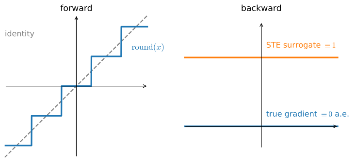
Zero gradient, exactly as calculus demands, and useless for training. The straight-through estimator (Bengio et al. 2013) resolves this with a controlled lie: keep the rounding in the forward pass, but pretend in the backward pass that it was the identity.
No automatic system can derive a lie for us, so we override the chain rule with torch.autograd.Function, supplying both directions ourselves as static methods. Figure 5.4.1 draws that split explicitly.
No automatic system can derive a lie for us, so we override the chain rule with @tf.custom_gradient, a decorator under which the function returns its backward rule alongside its output. Figure 5.4.1 draws that split explicitly.
No automatic system can derive a lie for us, so we override the chain rule with jax.custom_vjp, attaching a hand-written backward rule (a vector-Jacobian product) to an ordinary function. Figure 5.4.1 draws that split explicitly.
No automatic system can derive a lie for us, so we override the chain rule with autograd.Function, supplying both directions ourselves as methods of a class. Figure 5.4.1 draws that split explicitly.
class RoundSTE(torch.autograd.Function):
    @staticmethod
    def forward(ctx, X):
        return X.round()

    @staticmethod
    def backward(ctx, grad_output):
        # Pretend forward was the identity: pass the gradient straight through
        return grad_output
@tf.custom_gradient
def round_ste(X):
def grad(upstream):
# Pretend forward was the identity: pass the gradient straight through
return upstream
return tf.round(X), grad@jax.custom_vjp
def round_ste(X):
return jnp.round(X)
def round_ste_fwd(X):
return jnp.round(X), None # (output, residuals); we need no residuals
def round_ste_bwd(residuals, grad_output):
# Pretend forward was the identity: pass the gradient straight through
return (grad_output,)
round_ste.defvjp(round_ste_fwd, round_ste_bwd)class RoundSTE(autograd.Function):
def forward(self, X):
return np.round(X)
def backward(self, grad_output):
# Pretend forward was the identity: pass the gradient straight through
return grad_outputTwo rules govern the class. First, invoke it through RoundSTE.apply(X), never by calling forward directly: apply is what inserts the operation into the autograd graph, while a direct call computes the same values with no bookkeeping, and backward then never runs. Calling forward directly therefore omits the custom backward rule without raising an error. Second, backward receives the loss gradient with respect to the output and must return the gradient with respect to each input. Ours ignores the input values entirely; a backward that needs them must stash them in forward with ctx.save_for_backward and retrieve them from ctx.
Two rules govern the decorator. First, the decorated function returns a pair: the output and the gradient function. Because the gradient function is a closure defined inside the forward pass, it captures values such as the inputs that the backward computation needs. There is no separate residual mechanism, and the decorated function is invoked like any other function; the decorator handles the tape bookkeeping. Second, grad receives the loss gradient with respect to the output and must return one gradient per argument of the decorated function. State requires an additional interface: if the wrapped computation reads a tf.Variable, the gradient function must accept a variables keyword argument and return the variables’ gradients as a second result; TensorFlow raises a TypeError naming this requirement if it is missing.
Two rules govern the definition. First, the forward rule must return a pair: the output plus whatever residuals the backward rule will need. Ours needs nothing and returns None; returning the output alone instead produces a structure-mismatch error because the residual is missing. Second, the backward rule receives those residuals and the loss gradient with respect to the output, and must return a tuple holding one gradient per argument of the original function, hence (grad_output,) rather than grad_output. An argument that is not differentiable data, say a configuration flag, must be declared through nondiff_argnums so it is routed past the gradient machinery.
Two rules govern the class. First, a Function instance is single-use: the library asserts that each instance is called exactly once, so create a fresh RoundSTE() at every application rather than reusing one, or the second call fails with an assertion naming this rule. Second, backward receives the loss gradient with respect to each output of forward and must return the gradient with respect to each input. Ours ignores the input values entirely; a backward that needs them must stash them in forward with self.save_for_backward and read them back from self.saved_tensors.
A small example verifies that the gradient now flows. We multiply the rounded values by known weights, so we know what gradient to expect at w.
w.grad = None
y = (RoundSTE.apply(w) * torch.tensor([1.0, 2.0, 3.0])).sum()
y.backward()
w.grad
tensor([1., 2., 3.])with tf.GradientTape() as tape:
y = tf.reduce_sum(round_ste(w) * tf.constant([1.0, 2.0, 3.0]))
tape.gradient(y, w)<tf.Tensor: shape=(3,), dtype=float32, numpy=array([1., 2., 3.], dtype=float32)>jax.grad(lambda w: (round_ste(w) * jnp.array([1.0, 2.0, 3.0])).sum())(w)Array([1., 2., 3.], dtype=float32)with autograd.record():
y = (RoundSTE()(w) * np.array([1.0, 2.0, 3.0])).sum()
y.backward()
w.gradarray([1., 2., 3.])The downstream gradient arrives at w untouched, as if the rounding were the identity, while the forward pass still computed with rounded values. Some estimators instead zero the gradient where a saved input had saturated, while ordinary gradient clipping bounds a large upstream gradient independently of the quantizer. These are different approximations. Neither is a universal default; the surrogate backward rule must match the training objective it is meant to approximate.
JAX offers a shortcut for this particular lie. jax.lax.stop_gradient is an identity whose gradient is zero, so X + stop_gradient(round(X) - X) computes round(X) in the forward pass while the backward pass sees only the leading X. Three lines, no custom_vjp; the general mechanism earns its keep when the surrogate is not the identity, an input-dependent saturation rule for instance. The two definitions agree in value and in gradient:
def round_ste2(X):
    return X + jax.lax.stop_gradient(jnp.round(X) - X)

def loss(f, w):
    return (f(w) * jnp.array([1.0, 2.0, 3.0])).sum()

(bool(jnp.allclose(round_ste(w), round_ste2(w))),
 bool(jnp.allclose(jax.grad(loss, 1)(round_ste, w),
                   jax.grad(loss, 1)(round_ste2, w))))
(True, True)A scope note to close. A custom gradient redefines the gradient of a computation assembled from existing tensor operations; it does not create new ones. Writing new kernels, code that runs on the accelerator itself, is a separate craft that we do not cover in this book; Chapter 13 discusses how to get performance out of the operations you already have.
5.4.5 Summary
A custom layer is a module subclass: forward defines the computation, nn.Parameter registers learnable state, and register_buffer registers persistent state that no optimizer should touch. Registration provides parameter tracking, container compatibility, serialization, and device movement, as we verified on RMSNorm axis by axis. When the chain rule itself must be overridden, as in the straight-through estimator, torch.autograd.Function lets you supply forward and backward as a pair, invoked through apply. Custom implementations expose these mechanisms; framework-provided operations are preferable when they meet production requirements.
A custom layer is a layer subclass: call defines the computation, add_weight registers learnable state, and add_weight(trainable=False) registers persistent state that no optimizer should touch. Registration provides parameter tracking, container compatibility, and serialization, with device placement settled at creation, as the RMSNorm examples verified. When the chain rule itself must be overridden, as in the straight-through estimator, @tf.custom_gradient lets the forward function return its own backward rule. Custom implementations expose these mechanisms; framework-provided operations are preferable when they meet production requirements.
A custom layer is a module subclass: __call__ defines the computation, nnx.Param registers learnable state, and another nnx.Variable subclass registers persistent state that the optimizer does not touch. Registration provides parameter tracking, container compatibility, serialization, and device movement, as we verified on RMSNorm axis by axis. When the chain rule itself must be overridden, as in the straight-through estimator, jax.custom_vjp attaches a forward and a backward rule to a function, and jax.lax.stop_gradient covers the identity-surrogate case in a single expression. Custom implementations expose these mechanisms; framework-provided operations are preferable when they meet production requirements.
A custom layer is a block subclass: forward defines the computation, assigning a gluon.Parameter registers learnable state, and gluon.Constant registers persistent state that autograd and the Trainer ignore. Registration provides parameter tracking, container compatibility, serialization, and device movement, as the RMSNorm examples verified. When the chain rule itself must be overridden, as in the straight-through estimator, autograd.Function lets you supply forward and backward as a pair, one fresh instance per call. Custom implementations expose these mechanisms. Use framework-provided operations when they meet production requirements; where Gluon provides none, as with RMSNorm, maintain the custom implementation.
5.4.6 Exercises
- [code] RMSNorm bias. Add an optional learned bias \(\mathbf{b}\) to
RMSNorm(a shift applied after the scale, restoring part of what LayerNorm had), and verify that the state dict of a model containing it grows by the expected entry. Then place the layer directly before a linear layer with weight \(\mathbf{W}\) and bias \(\mathbf{c}\), and show that \(\mathbf{b}\) can be folded into \(\mathbf{c}\) without changing the outputs. What is the folded bias? - [code] Dropout from scratch. Implement
Dropoutas a custom layer that zeroes each entry with probability \(p\) and rescales the survivors during training, but is the identity during evaluation. Where does thetrainingflag yourforwardconsults live, and how does calling.eval()on an enclosingSequentialreach your layer? - [code] Custom gradients.
- Implement a clamp with a custom gradient: an
autograd.Functionwhose forward isX.clamp(lo, hi)and whose backward passes the gradient only where the input lay strictly inside the clamp range. Compare its gradients with those of the nativetorch.clampfor inputs inside, outside, and exactly on the boundary. Which convention does the native operation use at the boundary? - Implement a second custom operation, GELU or Softplus, with a hand-derived backward. Check it numerically against the automatic derivative of the equivalent built-in expression and report the largest discrepancy.
- Implement a clamp with a custom gradient: an
- [code] Offset causal mask. During cached decoding, the score matrix has shape \(T_q \times T_k\) with \(T_q \le T_k\), and the \(T_q\) queries occupy the last \(T_q\) of the \(T_k\) key positions. Generalize
CausalMaskto such score matrices while it still slices its single precomputedmax_len\(\times\)max_lentable. Check that the result agrees with the original layer when \(T_q = T_k\), state which entries it masks when \(T_q = 1\), and state what happens when \(T_k\) exceedsmax_len. - [extended] Bucketing with a straight-through estimator. ● Figure 5.4.1 passes a surrogate gradient through
round(x). Extend the idea to a layer whose forward pass maps a score \(s\) to the bucket index \(\lfloor K\sigma(s) \rfloor\) and whose backward pass treats the floor as the identity. Return the index as a floating-point tensor so that gradients can reach \(s\). Place the layer with \(K = 4\) between two linear layers of output width one, and train the network on inputs \(\mathbf{x} \in \mathbb{R}^{10}\) with targets \(y = \lfloor 4\sigma(\mathbf{w}^\top \mathbf{x}) \rfloor\) for a fixed random \(\mathbf{w}\). Compare the final training loss with that of the same network in which the floor keeps its true gradient, and explain which parameters learn in each case.
- [code] RMSNorm bias. Add an optional learned bias \(\mathbf{b}\) to
RMSNorm(a shift applied after the scale, restoring part of what LayerNorm had), and verify thatget_weightson a model containing it grows by the expected entry. Then place the layer directly before a linear layer with weight \(\mathbf{W}\) and bias \(\mathbf{c}\), and show that \(\mathbf{b}\) can be folded into \(\mathbf{c}\) without changing the outputs. What is the folded bias? - [code] Dropout from scratch. Implement
Dropoutas a custom layer that zeroes each entry with probability \(p\) and rescales the survivors during training, but is the identity during evaluation. Keras passes atrainingargument tocall; how does calling an enclosingSequentialwithtraining=Falsereach your layer? - [code] Custom gradients.
- Implement a clamp with a custom gradient: a
@tf.custom_gradientfunction whose forward istf.clip_by_value(X, lo, hi)and whose backward passes the gradient only where the input lay strictly inside the clamp range; the gradient closure must captureX. Compare its gradients with those of the nativetf.clip_by_valuefor inputs inside, outside, and exactly on the boundary. Which convention does the native operation use at the boundary? - Implement a second custom operation, GELU or Softplus, with a hand-derived backward. Check it numerically against the automatic derivative of the equivalent built-in expression and report the largest discrepancy.
- Implement a clamp with a custom gradient: a
- [code] Offset causal mask. During cached decoding, the score matrix has shape \(T_q \times T_k\) with \(T_q \le T_k\), and the \(T_q\) queries occupy the last \(T_q\) of the \(T_k\) key positions. Generalize
CausalMaskto such score matrices while it still slices its single precomputedmax_len\(\times\)max_lentable. Check that the result agrees with the original layer when \(T_q = T_k\), state which entries it masks when \(T_q = 1\), and state what happens when \(T_k\) exceedsmax_len. - [extended] Bucketing with a straight-through estimator. ● Figure 5.4.1 passes a surrogate gradient through
round(x). Extend the idea to a layer whose forward pass maps a score \(s\) to the bucket index \(\lfloor K\sigma(s) \rfloor\) and whose backward pass treats the floor as the identity. Return the index as a floating-point tensor so that gradients can reach \(s\). Place the layer with \(K = 4\) between two linear layers of output width one, and train the network on inputs \(\mathbf{x} \in \mathbb{R}^{10}\) with targets \(y = \lfloor 4\sigma(\mathbf{w}^\top \mathbf{x}) \rfloor\) for a fixed random \(\mathbf{w}\). Compare the final training loss with that of the same network in which the floor keeps its true gradient, and explain which parameters learn in each case.
- [code] RMSNorm bias. Add an optional learned bias \(\mathbf{b}\) to
RMSNorm(a shift applied after the scale, restoring part of what LayerNorm had), and verify that the parameter state of a model containing it grows by the expected entry. Then place the layer directly before a linear layer with weight \(\mathbf{W}\) and bias \(\mathbf{c}\), and show that \(\mathbf{b}\) can be folded into \(\mathbf{c}\) without changing the outputs. What is the folded bias? - [code] Dropout from scratch. Implement
Dropoutas a custom layer that zeroes each entry with probability \(p\) and rescales the survivors during training, but is the identity during evaluation. Give it thedeterministicflag, the RNG stream, and theset_viewmethod ofDropoutMLPScratch(Section 4.6). How does callingnnx.viewwithdeterministic=Trueon an enclosingnnx.Sequentialreach your layer? - [code] Custom gradients.
- Implement a clamp with a custom gradient: a
custom_vjpfunction whose forward isjnp.clip(X, lo, hi)and whose backward passes the gradient only where the input lay strictly inside the clamp range; the forward rule must saveXas a residual. Compare its gradients with those of the nativejnp.clipfor inputs inside, outside, and exactly on the boundary. Which convention does the native operation use at the boundary? - Implement a second custom operation, GELU or Softplus, with a hand-derived backward. Check it numerically against the automatic derivative of the equivalent built-in expression and report the largest discrepancy.
- Implement a clamp with a custom gradient: a
- [code] Offset causal mask. During cached decoding, the score matrix has shape \(T_q \times T_k\) with \(T_q \le T_k\), and the \(T_q\) queries occupy the last \(T_q\) of the \(T_k\) key positions. Generalize
CausalMaskto such score matrices while it still slices its single precomputedmax_len\(\times\)max_lentable. Check that the result agrees with the original layer when \(T_q = T_k\), state which entries it masks when \(T_q = 1\), and state what happens when \(T_k\) exceedsmax_len. - [extended] Bucketing with a straight-through estimator. ● Figure 5.4.1 passes a surrogate gradient through
round(x). Extend the idea to a layer whose forward pass maps a score \(s\) to the bucket index \(\lfloor K\sigma(s) \rfloor\) and whose backward pass treats the floor as the identity. Return the index as a floating-point tensor so that gradients can reach \(s\). Place the layer with \(K = 4\) between two linear layers of output width one, and train the network on inputs \(\mathbf{x} \in \mathbb{R}^{10}\) with targets \(y = \lfloor 4\sigma(\mathbf{w}^\top \mathbf{x}) \rfloor\) for a fixed random \(\mathbf{w}\). Compare the final training loss with that of the same network in which the floor keeps its true gradient, and explain which parameters learn in each case.
- [code] RMSNorm bias. Add an optional learned bias \(\mathbf{b}\) to
RMSNorm(a shift applied after the scale, restoring part of what LayerNorm had), and verify that the file written bysave_parametersfor a model containing it grows by the expected entry. Then place the layer directly before a linear layer with weight \(\mathbf{W}\) and bias \(\mathbf{c}\), and show that \(\mathbf{b}\) can be folded into \(\mathbf{c}\) without changing the outputs. What is the folded bias? - [code] Dropout from scratch. Implement
Dropoutas a custom layer that zeroes each entry with probability \(p\) and rescales the survivors during training, but is the identity during evaluation. Itsforwardconsultsautograd.is_training(), whichautograd.record()switches on together with recording (Section 5.2). Run the layer under all four combinations of recording and training mode, usingautograd.record(train_mode=False)andautograd.train_mode()for the mixed cases. For each combination, report whether entries are dropped and whether a gradient reaches the input. - [code] Custom gradients.
- Implement a clamp with a custom gradient: an
autograd.Functionwhose forward isnp.clip(X, lo, hi)and whose backward passes the gradient only where the input lay strictly inside the clamp range;forwardmust stashXwithsave_for_backward. Compare its gradients with those of the nativenp.clipfor inputs inside, outside, and exactly on the boundary. Which convention does the native operation use at the boundary? - Implement a second custom operation, GELU or Softplus, with a hand-derived backward. Check it numerically against the automatic derivative of the equivalent built-in expression and report the largest discrepancy.
- Implement a clamp with a custom gradient: an
- [code] Offset causal mask. During cached decoding, the score matrix has shape \(T_q \times T_k\) with \(T_q \le T_k\), and the \(T_q\) queries occupy the last \(T_q\) of the \(T_k\) key positions. Generalize
CausalMaskto such score matrices while it still slices its single precomputedmax_len\(\times\)max_lentable. Check that the result agrees with the original layer when \(T_q = T_k\), state which entries it masks when \(T_q = 1\), and state what happens when \(T_k\) exceedsmax_len. - [extended] Bucketing with a straight-through estimator. ● Figure 5.4.1 passes a surrogate gradient through
round(x). Extend the idea to a layer whose forward pass maps a score \(s\) to the bucket index \(\lfloor K\sigma(s) \rfloor\) and whose backward pass treats the floor as the identity. Return the index as a floating-point tensor so that gradients can reach \(s\). Place the layer with \(K = 4\) between two linear layers of output width one, and train the network on inputs \(\mathbf{x} \in \mathbb{R}^{10}\) with targets \(y = \lfloor 4\sigma(\mathbf{w}^\top \mathbf{x}) \rfloor\) for a fixed random \(\mathbf{w}\). Compare the final training loss with that of the same network in which the floor keeps its true gradient, and explain which parameters learn in each case.