1.4 Calculus

For a long time, how to calculate the area of a circle remained a mystery. Then, in Ancient Greece, the mathematician Archimedes came up with the clever idea to inscribe a series of polygons with increasing numbers of vertices on the inside of a circle (Figure 1.4.1). For a polygon with $n$ vertices, we obtain $n$ triangles. The height of each triangle approaches the radius $r$ as we partition the circle more finely. At the same time, its base approaches $2 \pi r/n$, since the ratio between arc and secant approaches 1 for a large number of vertices. Thus, the area of the polygon approaches $n \cdot r \cdot \frac{1}{2} (2 \pi r/n) = \pi r^2$.

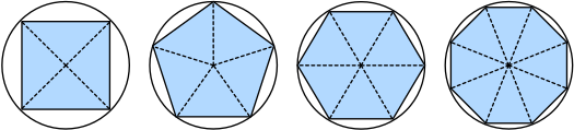
Figure 1.4.1: Finding the area of a circle as a limit procedure.

This limiting procedure is at the root of both differential calculus and integral calculus. The former can tell us how to increase or decrease a function’s value by manipulating its arguments. This comes in handy for the optimization problems that we face in deep learning, where we repeatedly update our parameters in order to decrease the loss function. Optimization addresses how to fit our models to training data, and calculus is its key prerequisite. However, do not forget that our ultimate goal is to perform well on previously unseen data. That problem is called generalization and will be a key focus of other chapters.

%matplotlib inline
from d2l import torch as d2l
from matplotlib_inline import backend_inline
import numpy as np

%matplotlib inline
from d2l import tensorflow as d2l
from matplotlib_inline import backend_inline
import numpy as np

%matplotlib inline
from d2l import jax as d2l
from matplotlib_inline import backend_inline
import numpy as np

%matplotlib inline
from d2l import mxnet as d2l
from matplotlib_inline import backend_inline
from mxnet import np, npx
npx.set_np()

1.4.1 Derivatives and Differentiation

Put simply, a derivative is the rate of change in a function with respect to changes in its arguments. Derivatives can tell us how rapidly a loss function would increase or decrease were we to increase or decrease each parameter by an infinitesimally small amount. Formally, for functions $f: \mathbb{R} \rightarrow \mathbb{R}$, that map from scalars to scalars, the derivative of $f$ at a point $x$ is defined as

\[f'(x) = \lim_{h \rightarrow 0} \frac{f(x+h) - f(x)}{h}. \tag{1.4.1}\]

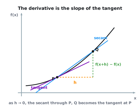
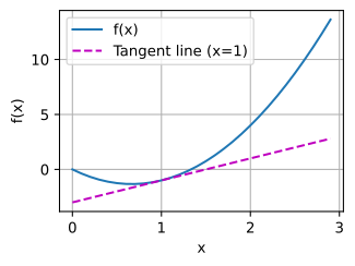
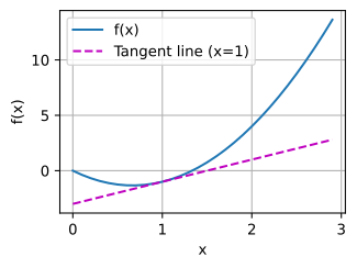
This term on the right hand side is called a limit and it tells us what happens to the value of an expression as a specified variable approaches a particular value. This limit tells us what the ratio between the change in the function value $f(x + h) - f(x)$ and the perturbation $h$ converges to as we shrink $h$ to zero. Geometrically, the difference quotient is the slope of the secant line through the points $(x, f(x))$ and $(x+h, f(x+h))$; as $h \rightarrow 0$, the secant pivots into the tangent line at $x$, whose slope is the derivative (Figure 1.4.2).

Figure 1.4.2: As $h \to 0$, the secant line through $P$ and $Q$ pivots into the tangent line at $P$: the derivative is the slope of the tangent.

When $f'(x)$ exists, $f$ is said to be differentiable at $x$; and when $f'(x)$ exists for all $x$ on a set, e.g., the interval $[a,b]$, we say that $f$ is differentiable on this set. Not all functions are differentiable, including many that we wish to optimize, such as classification accuracy. However, because nearly every algorithm for training deep neural networks must compute the derivative of the loss, we often optimize a differentiable surrogate instead.

We can interpret the derivative $f'(x)$ as the instantaneous rate of change of $f(x)$ with respect to $x$. Let’s develop some intuition with an example. Define $u = f(x) = 3x^2-4x$.

def f(x):
    return 3 * x ** 2 - 4 * x

def f(x):
    return 3 * x ** 2 - 4 * x

def f(x):
    return 3 * x ** 2 - 4 * x

def f(x):
    return 3 * x ** 2 - 4 * x

Setting $x=1$, we see that $\frac{f(x+h) - f(x)}{h}$ approaches $2$ as $h$ approaches $0$. While this experiment lacks the rigor of a mathematical proof, we can quickly see that indeed $f'(1) = 2$.

for h in 10.0**np.arange(-1, -6, -1):
    print(f'h={h:.5f}, numerical limit={(f(1+h)-f(1))/h:.5f}')

h=0.10000, numerical limit=2.30000
h=0.01000, numerical limit=2.03000
h=0.00100, numerical limit=2.00300
h=0.00010, numerical limit=2.00030
h=0.00001, numerical limit=2.00003

h=0.10000, numerical limit=2.30000
h=0.01000, numerical limit=2.03000
h=0.00100, numerical limit=2.00300
h=0.00010, numerical limit=2.00030
h=0.00001, numerical limit=2.00003

h=0.10000, numerical limit=2.30000
h=0.01000, numerical limit=2.03000
h=0.00100, numerical limit=2.00300
h=0.00010, numerical limit=2.00030
h=0.00001, numerical limit=2.00003

h=0.10000, numerical limit=2.30000
h=0.01000, numerical limit=2.02999
h=0.00100, numerical limit=2.00295
h=0.00010, numerical limit=2.00033
h=0.00001, numerical limit=2.00272

It is tempting to conclude that smaller $h$ is always better. Not so: in floating-point arithmetic, $f(x+h)$ and $f(x)$ become nearly equal numbers as $h$ shrinks, so their difference loses most of its significant digits to cancellation, and dividing by the tiny $h$ amplifies whatever rounding noise remains. Continuing the sweep to much smaller $h$ shows the approximation degrading and then failing outright: the error creeps into ever-higher digits, and once $h$ is so small that $1 + h$ rounds to exactly $1$, the quotient collapses to zero.

for exp in range(-6, -17, -1):
    h = 10.0 ** exp
    print(f'h={h:.0e}, numerical limit={(f(1+h)-f(1))/h:.5f}')

h=1e-06, numerical limit=2.00000
h=1e-07, numerical limit=2.00000
h=1e-08, numerical limit=2.00000
h=1e-09, numerical limit=2.00000
h=1e-10, numerical limit=2.00000
h=1e-11, numerical limit=2.00000
h=1e-12, numerical limit=2.00018
h=1e-13, numerical limit=1.99840
h=1e-14, numerical limit=1.99840
h=1e-15, numerical limit=2.22045
h=1e-16, numerical limit=0.00000

The numerical limit is thus caught between two error sources: truncation error (from $h$ being too large) and cancellation (from $h$ being too small). This is one important reason why the automatic differentiation introduced in Section 1.5 computes derivatives analytically, by applying differentiation rules, rather than by finite differences.

There are several equivalent notational conventions for derivatives. Given $y = f(x)$, the following expressions are equivalent:

\[f'(x) = y' = \frac{dy}{dx} = \frac{df}{dx} = \frac{d}{dx} f(x) = Df(x) = D_x f(x),\]

where the symbols $\frac{d}{dx}$ and $D$ are differentiation operators. Below, we present the derivatives of some common functions:

\[\begin{aligned} \frac{d}{dx} C & = 0 && \textrm{for any constant $C$} \\ \frac{d}{dx} x^n & = n x^{n-1} && \textrm{for } x > 0 \textrm{ if } n \textrm{ is not an integer} \\ \frac{d}{dx} e^x & = e^x \\ \frac{d}{dx} \ln x & = x^{-1}. \end{aligned} \tag{1.4.2}\]

Functions composed from differentiable functions are often themselves differentiable. The following rules cover compositions of any differentiable functions $f$ and $g$, and constant $C$.

\[\begin{aligned} \frac{d}{dx} [C f(x)] & = C \frac{d}{dx} f(x) && \textrm{Constant multiple rule} \\ \frac{d}{dx} [f(x) + g(x)] & = \frac{d}{dx} f(x) + \frac{d}{dx} g(x) && \textrm{Sum rule} \\ \frac{d}{dx} [f(x) g(x)] & = f(x) \frac{d}{dx} g(x) + g(x) \frac{d}{dx} f(x) && \textrm{Product rule} \\ \frac{d}{dx} \frac{f(x)}{g(x)} & = \frac{g(x) \frac{d}{dx} f(x) - f(x) \frac{d}{dx} g(x)}{g^2(x)} && \textrm{Quotient rule} \end{aligned} \tag{1.4.3}\]

Using this, we can apply the rules to find the derivative of $3 x^2 - 4x$ via

\[\frac{d}{dx} [3 x^2 - 4x] = 3 \frac{d}{dx} x^2 - 4 \frac{d}{dx} x = 6x - 4. \tag{1.4.4}\]

Plugging in $x = 1$ shows that, indeed, the derivative equals $2$ at this location. We state these derivatives and rules without proof for now; each follows from the limit definition, as shown in Section 24.1, which also collects a longer table of common derivatives. Note that derivatives tell us the slope of a function at a particular location.

We can make that slope visible by plotting the function $u = f(x)$ together with its tangent line $y = 2x - 3$ at $x=1$, where the coefficient $2$ is the slope of the tangent line. We use d2l.plot, one of a handful of matplotlib helpers that we define at the end of this section and reuse throughout the book.

x = np.arange(0, 3, 0.1)
d2l.plot(x, [f(x), 2 * x - 3], 'x', 'f(x)', legend=['f(x)', 'Tangent line (x=1)'])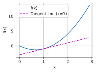

1.4.2 Partial Derivatives and Gradients

Thus far, we have been differentiating functions of just one variable. In deep learning, we also need to work with functions of many variables, typically functions that take the vectors and matrices from Section 1.3 as their inputs. We briefly introduce notions of the derivative that apply to such multivariate functions.

Let $y = f(x_1, x_2, \ldots, x_n)$ be a function with $n$ variables. The partial derivative of $y$ with respect to its $i^\textrm{th}$ parameter $x_i$ is

\[ \frac{\partial y}{\partial x_i} = \lim_{h \rightarrow 0} \frac{f(x_1, \ldots, x_{i-1}, x_i+h, x_{i+1}, \ldots, x_n) - f(x_1, \ldots, x_i, \ldots, x_n)}{h}. \tag{1.4.5}\]

To calculate $\frac{\partial y}{\partial x_i}$, we can treat $x_1, \ldots, x_{i-1}, x_{i+1}, \ldots, x_n$ as constants and calculate the derivative of $y$ with respect to $x_i$. The following notational conventions for partial derivatives are all common and all mean the same thing:

\[\frac{\partial y}{\partial x_i} = \frac{\partial f}{\partial x_i} = \partial_{x_i} f = \partial_i f = f_{x_i} = f_i = D_i f = D_{x_i} f. \tag{1.4.6}\]

We can concatenate partial derivatives of a multivariate function with respect to all its variables to obtain a vector that is called the gradient of the function. Suppose that the input of function $f: \mathbb{R}^n \rightarrow \mathbb{R}$ is an $n$-dimensional vector $\mathbf{x} = [x_1, x_2, \ldots, x_n]^\top$ and the output is a scalar. The gradient of the function $f$ with respect to $\mathbf{x}$ is a vector of $n$ partial derivatives:

\[\nabla_{\mathbf{x}} f(\mathbf{x}) = \left[\partial_{x_1} f(\mathbf{x}), \partial_{x_2} f(\mathbf{x}), \ldots, \partial_{x_n} f(\mathbf{x})\right]^\top. \tag{1.4.7}\]

When there is no ambiguity, $\nabla_{\mathbf{x}} f(\mathbf{x})$ is typically replaced by $\nabla f(\mathbf{x})$.

What if we move away from $\mathbf{x}$ in an arbitrary unit direction $\mathbf{u}$, rather than along a coordinate axis? The rate of change of $f$ along $\mathbf{u}$ is called the directional derivative; for differentiable $f$ it equals the dot product $\nabla f(\mathbf{x})^\top \mathbf{u}$, an identity shown in Section 24.2. By the cosine formula for dot products from Section 1.3, this is largest when $\mathbf{u}$ aligns with the gradient.

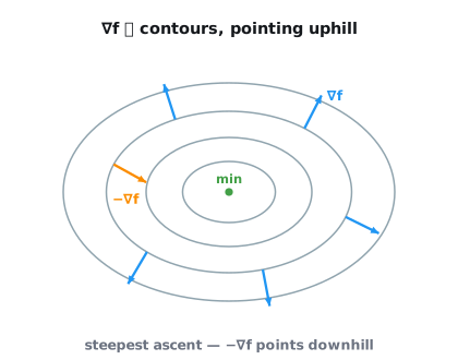
Hence the gradient has a geometric interpretation: it points in the direction of steepest ascent of $f$, i.e., the direction in which the function grows fastest (a claim proved via the Cauchy–Schwarz inequality in Section 24.2). To decrease $f$ as quickly as possible we therefore take a small step in the opposite direction, along the negative gradient $-\nabla f(\mathbf{x})$. This is the idea behind gradient descent, which takes a small step along $-\nabla f$. Later optimizers modify this direction using momentum, coordinatewise scaling, or curvature information, but the gradient remains the local signal from which their updates are constructed. Figure 1.4.3 shows the picture to keep in mind: gradients are perpendicular to the level sets of $f$ (the curves along which $f$ is constant) and point uphill, so $-\nabla f$ points downhill.

Figure 1.4.3: Level sets of a function with its gradient field: $\nabla f$ is perpendicular to the contours and points uphill, so $-\nabla f$ is the direction of steepest descent.

The following rules for differentiating multivariate functions recur throughout the book. The first involves a vector-valued function $\mathbf{u} = \mathbf{A}\mathbf{x}$: here we collect the partial derivatives $\partial u_j / \partial x_i$ into a matrix, and by convention we write $\nabla_{\mathbf{x}} \mathbf{A} \mathbf{x} = \mathbf{A}^\top$ (the transpose of the Jacobian, developed in Section 24.3).

For $\mathbf{A} \in \mathbb{R}^{m \times n}$ we have $\nabla_{\mathbf{x}} \mathbf{A} \mathbf{x} = \mathbf{A}^\top$; for $\mathbf{A} \in \mathbb{R}^{n \times m}$ we have $\nabla_{\mathbf{x}} \mathbf{x}^\top \mathbf{A} = \mathbf{A}$.
For square matrices $\mathbf{A} \in \mathbb{R}^{n \times n}$ we have that $\nabla_{\mathbf{x}} \mathbf{x}^\top \mathbf{A} \mathbf{x} = (\mathbf{A} + \mathbf{A}^\top)\mathbf{x}$ and in particular $\nabla_{\mathbf{x}} \|\mathbf{x} \|^2 = \nabla_{\mathbf{x}} \mathbf{x}^\top \mathbf{x} = 2\mathbf{x}$.

Similarly, for any matrix $\mathbf{X}$, we have $\nabla_{\mathbf{X}} \|\mathbf{X} \|_\textrm{F}^2 = 2\mathbf{X}$. These identities (and many more) are derived in Section 24.3.

1.4.3 Chain Rule

In deep learning, the gradients of concern are often difficult to calculate because we are working with deeply nested functions (of functions (of functions…)). Fortunately, the chain rule takes care of this. Returning to functions of a single variable, suppose that $y = f(g(x))$ and that the underlying functions $y=f(u)$ and $u=g(x)$ are both differentiable. The chain rule states that

\[\frac{dy}{dx} = \frac{dy}{du} \frac{du}{dx}. \tag{1.4.8}\]

Turning back to multivariate functions, suppose that $y = f(\mathbf{u})$ has variables $u_1, u_2, \ldots, u_m$, where each $u_i = g_i(\mathbf{x})$ has variables $x_1, x_2, \ldots, x_n$, i.e., $\mathbf{u} = g(\mathbf{x})$. Then the chain rule states that

\[\frac{\partial y}{\partial x_{i}} = \frac{\partial y}{\partial u_{1}} \frac{\partial u_{1}}{\partial x_{i}} + \frac{\partial y}{\partial u_{2}} \frac{\partial u_{2}}{\partial x_{i}} + \ldots + \frac{\partial y}{\partial u_{m}} \frac{\partial u_{m}}{\partial x_{i}} \ \textrm{ and so } \ \nabla_{\mathbf{x}} y = \mathbf{A} \nabla_{\mathbf{u}} y, \tag{1.4.9}\]

where $\mathbf{A} \in \mathbb{R}^{n \times m}$ is the matrix whose entry $A_{ij} = \partial u_j / \partial x_i$ collects the derivatives of the components of $\mathbf{u}$ with respect to those of $\mathbf{x}$. Reading off the sum on the left, $(\nabla_{\mathbf{x}} y)_i = \sum_{j} A_{ij} (\nabla_{\mathbf{u}} y)_j$, which is exactly the matrix–vector product on the right. Thus, evaluating the gradient requires computing a matrix–vector product. This is one reason why linear algebra is a prerequisite for deep learning.

1.4.3.1 Plotting Utilities for This Book

Earlier we plotted a function and its tangent line with d2l.plot. Here is the small set of matplotlib helpers behind it, which the book reuses whenever it draws a curve. The #@save comment is a special modifier that stores a function, class, or code block in the d2l package, so that later sections can invoke it (e.g., as d2l.plot) without repeating the code. use_svg_display requests crisp SVG output, set_figsize sets the figure size, and set_axes configures labels, ranges, and scales. You do not need to study these; skim and move on.

def use_svg_display():
    """Use the svg format to display a plot in Jupyter."""
    backend_inline.set_matplotlib_formats('svg')

def set_figsize(figsize=(3.5, 2.5)):
    """Set the figure size for matplotlib."""
    use_svg_display()
    d2l.plt.rcParams['figure.figsize'] = figsize

def set_axes(axes, xlabel, ylabel, xlim, ylim, xscale, yscale, legend):
    """Set the axes for matplotlib."""
    axes.set_xlabel(xlabel), axes.set_ylabel(ylabel)
    axes.set_xscale(xscale), axes.set_yscale(yscale)
    axes.set_xlim(xlim),     axes.set_ylim(ylim)
    if legend:
        axes.legend(legend)
    axes.grid()

Finally, plot overlays multiple curves; most of its body just aligns the shapes of its inputs.

def plot(X, Y=None, xlabel=None, ylabel=None, legend=None, xlim=None,
         ylim=None, xscale='linear', yscale='linear',
         fmts=('-', 'm--', 'g-.', 'r:'), figsize=(3.5, 2.5), axes=None):
    """Plot data points."""
    legend = [] if legend is None else legend

    def has_one_axis(X):  # True if X (tensor or list) has 1 axis
        return (hasattr(X, "ndim") and X.ndim == 1 or isinstance(X, list)
                and not hasattr(X[0], "__len__"))
    
    if has_one_axis(X): X = [X]
    if Y is None:
        X, Y = [[]] * len(X), X
    elif has_one_axis(Y):
        Y = [Y]
    if len(X) != len(Y):
        X = X * len(Y)
        
    set_figsize(figsize)
    if axes is None:
        axes = d2l.plt.gca()
    axes.cla()
    for x, y, fmt in zip(X, Y, fmts):
        axes.plot(x,y,fmt) if len(x) else axes.plot(y,fmt)
    set_axes(axes, xlabel, ylabel, xlim, ylim, xscale, yscale, legend)

1.4.4 Discussion

Three ideas from this section recur throughout the book. First, and most important for what follows: from the viewpoint of optimization, the gradient tells us how to move the parameters of a model in order to lower the loss. Because $-\nabla f$ points in the direction of steepest descent, each step of the optimization algorithms used throughout this book amounts to evaluating the gradient and taking a short step along $-\nabla f$. Second, the composition rules for differentiation can be applied routinely, enabling us to compute gradients automatically; this task requires no creativity, so we can focus our cognitive powers elsewhere. Third, computing the derivatives of vector-valued functions requires us to multiply matrices as we trace the dependency graph of variables from output to input. Applying the chain rule backward through that graph is backpropagation, automated in Section 1.5 and developed in Section 4.3.

This section deliberately previews only the calculus we need to train models. For a thorough development (single- and multivariable calculus, the integral, and the matrix calculus behind automatic differentiation), see Chapter 24; Deisenroth et al. (2020) give a complementary treatment aimed at machine learning.

1.4.5 Exercises

So far we took the rules for derivatives for granted. Using the definition and limits prove the properties for (i) $f(x) = c$, (ii) $f(x) = x^n$, (iii) $f(x) = e^x$ and (iv) $f(x) = \log x$.
In the same vein, prove the product, sum, and quotient rule from first principles.
Prove that the constant multiple rule follows as a special case of the product rule.
Calculate the derivative of $f(x) = x^x$.
What does it mean that $f'(x) = 0$ for some $x$? Give an example of a function $f$ and a location $x$ for which this might hold.
Plot the function $y = f(x) = x^3 - \frac{1}{x}$ and plot its tangent line at $x = 1$.
Find the gradient of the function $f(\mathbf{x}) = 3x_1^2 + 5e^{x_2}$.
What is the gradient of the function $f(\mathbf{x}) = \|\mathbf{x}\|_2$? What happens for $\mathbf{x} = \mathbf{0}$?
Can you write out the chain rule for the case where $u = f(x, y, z)$ and $x = x(a, b)$, $y = y(a, b)$, and $z = z(a, b)$?
Given a function $f(x)$ that is invertible, compute the derivative of its inverse $f^{-1}(x)$. Here we have that $f^{-1}(f(x)) = x$ and conversely $f(f^{-1}(y)) = y$. Hint: use these properties in your derivation.
Consider the function $f(\mathbf{x}) = \|\mathbf{x}\|_2^2$. Starting from $\mathbf{x} = [1, 1]^\top$, take a single gradient-descent step $\mathbf{x} \leftarrow \mathbf{x} - \eta \nabla f(\mathbf{x})$ with learning rate $\eta = 0.1$ and verify that $f$ decreases. What happens if you instead pick $\eta = 1$? And $\eta = 2$? What does this tell you about the role of the learning rate?

Discussions