%matplotlib inline
from d2l import torch as d2l
import math
import torch
from torch import nn
from torch.nn import functional as F10.4 Positional Information
Without positional information, attention is permutation equivariant: reordering the input only reorders the output. This is unsuitable for sequences in which order changes meaning. This section proves the equivariance property and then studies four ways to represent position: sinusoidal and learned absolute embeddings, rotary position embeddings (RoPE), linear attention biases (ALiBi), and causal attention without explicit position embeddings (NoPE). We compare the methods both within the training context length and beyond it using a small character-level language model whose only cross-position operation is attention.
%matplotlib inline
from d2l import jax as d2l
from flax import nnx
import jax
from jax import numpy as jnp
import math
import optax
10.4.1 Attention Ignores Order
Let \(\mathbf{X} \in \mathbb{R}^{n \times d}\) hold a sequence of \(n\) token representations. At evaluation time, with dropout disabled and with no mask or position-dependent bias, let \(f\) be the self-attention layer
\[ f(\mathbf{X}) = \mathrm{softmax}\!\left(\frac{\mathbf{X}\mathbf{W}_q (\mathbf{X}\mathbf{W}_k)^\top}{\sqrt{d}}\right) \mathbf{X}\mathbf{W}_v. \tag{10.4.1}\]
Proposition (permutation equivariance). For every permutation matrix \(\boldsymbol{\Pi}\), \(\;f(\boldsymbol{\Pi} \mathbf{X}) = \boldsymbol{\Pi} f(\mathbf{X})\).
Proof. The projections act on each row separately, so \((\boldsymbol{\Pi}\mathbf{X})\mathbf{W} = \boldsymbol{\Pi}(\mathbf{X}\mathbf{W})\) for each of \(\mathbf{W}_q, \mathbf{W}_k, \mathbf{W}_v\). The score matrix becomes \(\boldsymbol{\Pi} \mathbf{S} \boldsymbol{\Pi}^\top\), and since softmax normalizes each row by itself, it commutes with row and column permutations: \(\mathrm{softmax}(\boldsymbol{\Pi} \mathbf{S} \boldsymbol{\Pi}^\top) = \boldsymbol{\Pi}\, \mathrm{softmax}(\mathbf{S})\, \boldsymbol{\Pi}^\top\). Multiplying by the permuted values, \(\boldsymbol{\Pi}\, \mathrm{softmax}(\mathbf{S})\, \boldsymbol{\Pi}^\top \boldsymbol{\Pi} \mathbf{X}\mathbf{W}_v = \boldsymbol{\Pi} f(\mathbf{X})\) because \(\boldsymbol{\Pi}^\top \boldsymbol{\Pi} = \mathbf{I}\). Concatenating heads and applying \(\mathbf{W}_o\) row-wise preserves the property, so it holds for multi-head attention too. \(\blacksquare\)
Permuting the input applies the same permutation to the output: each token’s output is unchanged except for its row index. Thus the layer does not use a token’s position in the sequence. We can verify this property on the multi-head layer of Section 10.3:
torch.manual_seed(0)
attention = d2l.MultiHeadAttention(num_hiddens=64, num_heads=4, dropout=0)
X = torch.randn(1, 8, 64)
perm = torch.randperm(8)
Y, Y_perm = attention(X, X, X, None), attention(X[:, perm], X[:, perm],
                                                X[:, perm], None)
print(f'max |Y[perm] - Y_perm|: {(Y[:, perm] - Y_perm).abs().max():.2e}')
max |Y[perm] - Y_perm|: 6.33e-08attention = d2l.MultiHeadAttention(num_hiddens=64, num_heads=4, dropout=0)
X = jax.random.normal(jax.random.key(0), (1, 8, 64))
perm = jax.random.permutation(jax.random.key(1), 8)
Y = attention(X, X, X, None)[0]
Y_perm = attention(X[:, perm], X[:, perm], X[:, perm], None)[0]
print(f'max |Y[perm] - Y_perm|: {jnp.abs(Y[:, perm] - Y_perm).max():.2e}')max |Y[perm] - Y_perm|: 0.00e+00Two caveats qualify this result. First, equivariance is a property of the layer; stacking equivariant layers and reading out per token leaves the model equivariant, so depth does not help. Second, the proposition is about unmasked attention: a causal mask singles out each position by how many predecessors it may see, which breaks the symmetry. NoPE uses this asymmetry, as discussed near the end of the section. The other methods provide each token with explicit positional information.
10.4.2 Absolute Position Embeddings
The original transformer attaches a position vector \(\mathbf{p}_i \in \mathbb{R}^d\) to each position \(i\) and feeds \(\mathbf{x}_i + \mathbf{p}_i\) into the first layer (Vaswani et al. 2017). Two tokens with identical embeddings at different positions now enter attention as different vectors, and the equivariance proof fails at its first step. The two classic choices of \(\mathbf{P}\) differ in whether the table is designed or learned.
10.4.2.1 Sinusoidal Encodings
The designed choice fills row \(i\) of \(\mathbf{P} \in \mathbb{R}^{n \times d}\) with sines and cosines of geometrically spaced frequencies,
\[ p_{i, 2j} = \sin\left(\frac{i}{10000^{2j/d}}\right), \qquad p_{i, 2j+1} = \cos\left(\frac{i}{10000^{2j/d}}\right). \tag{10.4.2}\]
The design looks arbitrary until you plot it. We implement the table as a small function and look at four adjacent columns:
def sinusoidal_encoding(max_len, num_hiddens):
    theta = torch.arange(max_len)[:, None] / 10000 ** (
        torch.arange(0, num_hiddens, 2) / num_hiddens)
    return torch.stack([torch.sin(theta), torch.cos(theta)],
                       -1).reshape(max_len, num_hiddens)

P = sinusoidal_encoding(60, 32)
d2l.plot(torch.arange(60), P[:, 6:10].T, xlabel='position',
         figsize=(6, 2.5), legend=[f'column {d}' for d in range(6, 10)])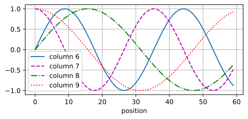
def sinusoidal_encoding(max_len, num_hiddens):
    theta = jnp.arange(max_len)[:, None] / 10000 ** (
        jnp.arange(0, num_hiddens, 2) / num_hiddens)
    return jnp.stack([jnp.sin(theta), jnp.cos(theta)],
                     -1).reshape(max_len, num_hiddens)

P = sinusoidal_encoding(60, 32)
d2l.plot(jnp.arange(60), P[:, 6:10].T, xlabel='position',
         figsize=(6, 2.5), legend=[f'column {d}' for d in range(6, 10)])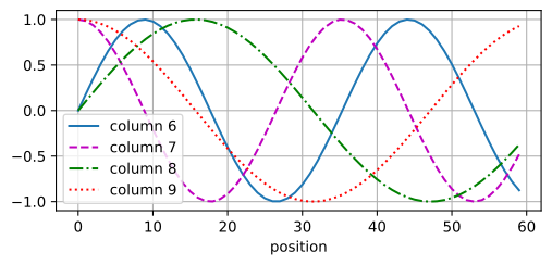
Adjacent column pairs share a frequency (one sine, one cosine), and the frequency falls as the column index grows. This is a continuous version of something familiar: binary counting. In the binary representations below, the lowest bit flips every number, the next every two numbers, the next every four. Fast dimensions distinguish neighboring positions, whereas slow dimensions distinguish broader regions:
for i in range(8):
    print(f'{i} in binary is {i:>03b}')
0 in binary is 000
1 in binary is 001
2 in binary is 010
3 in binary is 011
4 in binary is 100
5 in binary is 101
6 in binary is 110
7 in binary is 111The heatmap of the whole table shows the same structure in continuous form: each row is a unique multi-frequency fingerprint of its position, and unlike bits, the values vary smoothly, so nearby positions get nearby encodings.
d2l.show_heatmaps(P[None, None], xlabel='column (encoding dimension)',
                  ylabel='row (position)', figsize=(3.5, 4), cmap='Blues')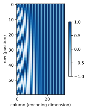
d2l.show_heatmaps(P[None, None], xlabel='column (encoding dimension)',
                  ylabel='row (position)', figsize=(3.5, 4), cmap='Blues')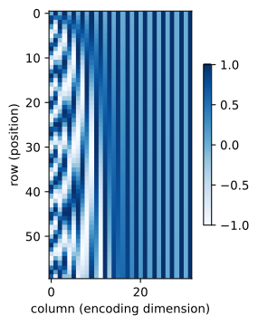
10.4.2.2 Learned Positions
The empirical choice is to make \(\mathbf{P}\) a trainable embedding table, one free vector per position, as in BERT and GPT-2 (Devlin et al. 2018; Radford et al. 2019). It concedes that we do not know the right encoding and lets gradient descent find one. The limitation is apparent before training: the table has exactly as many rows as the training context, and a row that no training example ever used is still whatever initialization left there. Position 500 is not “a bit beyond position 128”; it is undefined.
10.4.2.3 Sinusoidal Encodings as Rotations
Designed sinusoids have a relative-position structure absent from a learned table. The original paper observed that “for any fixed offset \(\delta\), \(\mathbf{p}_{i+\delta}\) is a linear function of \(\mathbf{p}_i\)”. The linear map can be written explicitly. Write \(\omega_j = 1/10000^{2j/d}\) for the frequency shared by columns \(2j\) and \(2j{+}1\). Then
\[ \begin{bmatrix} \cos(\delta \omega_j) & \sin(\delta \omega_j) \\ -\sin(\delta \omega_j) & \cos(\delta \omega_j) \\ \end{bmatrix} \begin{bmatrix} p_{i, 2j} \\ p_{i, 2j+1} \\ \end{bmatrix} = \begin{bmatrix} \sin\left((i+\delta) \omega_j\right) \\ \cos\left((i+\delta) \omega_j\right) \\ \end{bmatrix} = \begin{bmatrix} p_{i+\delta, 2j} \\ p_{i+\delta, 2j+1} \\ \end{bmatrix}, \tag{10.4.3}\]
by the angle-addition identities. The map from position \(i\) to position \(i + \delta\) is a rotation of each two-column pair, by an angle \(\delta \omega_j\) that depends only on the offset \(\delta\), never on \(i\). Thus the encoding contains relative-position structure, but only implicitly. The model receives \(\mathbf{x}_i + \mathbf{p}_i\) and must learn projections that exploit the rotations. Moreover, a query–key product of two such sums expands into four terms, and only the position–position term retains the rotation directly. RoPE instead applies relative rotations directly to the query–key comparison.
10.4.3 Rotary Position Embeddings
This construction is used by many current open-weights language models, including Llama, Qwen, and DeepSeek. Rotary position embeddings (RoPE) (Su et al. 2024) skip the addition and instead act on queries and keys at the point where they meet: the score. We want a transformation \(\mathbf{R}_i\), applied to the query at position \(i\) and the key at position \(j\), such that the score depends only on the content vectors and the offset \(j - i\):
\[ (\mathbf{R}_i \mathbf{q})^\top (\mathbf{R}_j \mathbf{k}) = \mathbf{q}^\top \mathbf{R}_i^\top \mathbf{R}_j \mathbf{k} \overset{!}{=} \mathbf{q}^\top \mathbf{R}_{j-i} \mathbf{k}. \tag{10.4.4}\]
The requirement \(\mathbf{R}_i^\top \mathbf{R}_j = \mathbf{R}_{j-i}\) says that the \(\mathbf{R}_i\) form a one-parameter group of orthogonal maps. Planar rotations satisfy this condition, so RoPE reuses the sinusoidal frequencies \(\omega_m\), but multiplicatively: split the \(d\) query dimensions into \(d/2\) pairs, and rotate pair \(m\) of the position-\(i\) query by the angle \(i\,\omega_m\) (and likewise for keys),
\[ \mathbf{R}_i = \begin{bmatrix} R(i\omega_0) & & \\ & \ddots & \\ & & R(i\omega_{d/2-1}) \end{bmatrix}, \qquad R(\alpha) = \begin{bmatrix} \cos\alpha & -\sin\alpha \\ \sin\alpha & \cos\alpha \end{bmatrix}. \tag{10.4.5}\]
Figure 10.4.1 shows one pair plane: shifting both positions by the same amount rotates query and key together, preserving their angle and dot product. The score therefore depends on position only through the offset. The construction has two additional properties: rotations preserve norms, so RoPE never inflates or shrinks a token’s content, and the geometric frequency ladder means low-frequency pairs rotate only slightly across a sentence while high-frequency pairs discriminate neighboring positions sharply. Every pair still carries content; the frequency ladder only controls how quickly position rotates it. Only queries and keys are rotated; values pass through untouched. (Learned relative-position embeddings (Shaw et al. 2018; Huang et al. 2018) pursued the same goal by adding trained offset vectors into the score; RoPE achieves relative scoring without additional learned parameters.)
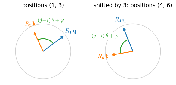
The implementation rotates the even/odd feature pairs with precomputed sines and cosines; offset shifts every position by the same amount, which we will use to test the invariance:
def rope(x, offset=0):
    """Rotate feature pairs of x (..., num_steps, d) by position angles."""
    d = x.shape[-1]
    pos = torch.arange(x.shape[-2], dtype=torch.float32,
                       device=x.device) + offset
    inv_freq = 10000.0 ** (-torch.arange(0, d, 2, device=x.device) / d)
    theta = pos[:, None] * inv_freq[None, :]
    cos, sin = torch.cos(theta), torch.sin(theta)
    x1, x2 = x[..., 0::2], x[..., 1::2]
    return torch.stack([x1 * cos - x2 * sin,
                        x1 * sin + x2 * cos], -1).flatten(-2)
def rope(x, offset=0):
"""Rotate feature pairs of x (..., num_steps, d) by position angles."""
d = x.shape[-1]
pos = jnp.arange(x.shape[-2], dtype=jnp.float32) + offset
inv_freq = 10000.0 ** (-jnp.arange(0, d, 2) / d)
theta = pos[:, None] * inv_freq[None, :]
cos, sin = jnp.cos(theta), jnp.sin(theta)
x1, x2 = x[..., 0::2], x[..., 1::2]
return jnp.stack([x1 * cos - x2 * sin,
x1 * sin + x2 * cos], -1).reshape(x.shape)A numerical check of Equation 10.4.4 shifts all positions jointly. The full RoPE score matrix should remain unchanged. For contrast, we run the same test on the additive sinusoidal encoding, where the four-term expansion leaves absolute position in the score:
torch.manual_seed(0)
T, d = 32, 64
q, k = torch.randn(T, d), torch.randn(T, d)

scores = lambda off: rope(q, off) @ rope(k, off).T / math.sqrt(d)
for off in (1, 17, 480):
    print(f'RoPE, all positions shifted by {off:>3}: max score change '
          f'{(scores(off) - scores(0)).abs().max():.1e}')

P = sinusoidal_encoding(600, d)
added = lambda off: (q + P[off:off+T]) @ (k + P[off:off+T]).T / math.sqrt(d)
print(f'additive sinusoidal, shifted by  17: max score change '
      f'{(added(17) - added(0)).abs().max():.1e}')
RoPE, all positions shifted by 1: max score change 1.7e-06
RoPE, all positions shifted by 17: max score change 1.5e-06
RoPE, all positions shifted by 480: max score change 1.4e-05
additive sinusoidal, shifted by 17: max score change 2.8e+00T, d = 32, 64
key1, key2 = jax.random.split(jax.random.key(0))
q, k = jax.random.normal(key1, (T, d)), jax.random.normal(key2, (T, d))
scores = lambda off: rope(q, off) @ rope(k, off).T / math.sqrt(d)
for off in (1, 17, 480):
print(f'RoPE, all positions shifted by {off:>3}: max score change '
f'{jnp.abs(scores(off) - scores(0)).max():.1e}')
P = sinusoidal_encoding(600, d)
added = lambda off: (q + P[off:off+T]) @ (k + P[off:off+T]).T / math.sqrt(d)
print(f'additive sinusoidal, shifted by 17: max score change '
f'{jnp.abs(added(17) - added(0)).max():.1e}')RoPE, all positions shifted by 1: max score change 1.5e-03
RoPE, all positions shifted by 17: max score change 1.7e-03
RoPE, all positions shifted by 480: max score change 1.8e-03
additive sinusoidal, shifted by 17: max score change 3.3e+00RoPE’s scores are unchanged up to floating-point round-off (three or more orders of magnitude below the score scale in these runs) at every shift, including one far beyond where any additive table would end; the additive encoding moves the scores by an amount comparable to the scores themselves. Relative position is therefore encoded by the architecture rather than learned from data. This property does not guarantee accurate predictions at offsets absent from the training data, which the next experiment tests.
10.4.4 Extrapolation Beyond the Training Length
Every scheme above fixes permutation blindness at the training length. They differ when evaluated outside the training range. A length-extrapolation test trains at context \(L\) and compares perplexity at \(L\) with perplexity at, for example, \(4L\). Two more schemes were designed for this setting.
10.4.4.1 ALiBi and NoPE
ALiBi (attention with linear biases) (Press et al. 2022) encodes no positions at all. It instead subtracts a distance penalty from every attention score: for query position \(i\) and key position \(j \leq i\) in head \(h\) of \(H\),
\[ \mathrm{score}_{ij} = \frac{\mathbf{q}_i^\top \mathbf{k}_j}{\sqrt{d}} - m_h\,(i - j), \qquad m_h = 2^{-8h/H}. \tag{10.4.6}\]
Each head discounts distant tokens at its own geometric rate. Head 1 uses a steep penalty and head \(H\) a much smaller one; the slope formula \(2^{-8h/H}\) is the paper’s choice for head counts that are powers of two, with other \(H\) interpolating the same geometric sequence. The bias depends only on distance, so it is defined for every context length, and a distance of 400 remains a valid input to the bias rather than an unallocated table index. The cost is a fixed recency prior the model cannot fully unlearn.
NoPE (no positional encoding) uses the asymmetry omitted from the proposition (Kazemnejad et al. 2023): a causal model can omit explicit position representations. The mask already breaks the symmetry — position 0 attends over one token, position 100 over a hundred and one — so the number of tokens competing in each softmax is itself positional information, and a decoder can in principle recover relative order from it. Because it uses neither a table nor a rotation, NoPE has no explicit position range. Its effectiveness depends on how much usable positional signal the mask supplies.
10.4.4.2 An Attention-Only Language Model
We compare extrapolation by training a deliberately minimal model that is also analyzed later in the chapter: a token embedding, a stack of residual causal attention blocks, and an output head tied to the embedding (Press and Wolf 2017). There is no feed-forward network and no normalization layer, and the attention projections carry no bias terms by default (a bias switch restores them; Section 10.6 has one use for it). Besides the embedding table, which doubles as the output head, attention is the only trainable cross-position operation. All mixing across positions therefore passes through attention, which makes the model easier to analyze in Section 10.6. It is the attention-only cousin of the TinyLM of Section 9.6.2, and the positional scheme is a constructor argument taking 'learned', 'sinusoidal', 'rope', 'alibi', or 'none', implemented exactly as in the equations above.
class TinyCharLM(nn.Module):
    """Attention-only character-level language model."""
    def __init__(self, vocab_size, num_hiddens=128, num_heads=4, num_blks=2,
                 pos='rope', max_len=512, bias=False):
        super().__init__()
        self.num_heads, self.pos = num_heads, pos
        self.token_emb = nn.Embedding(vocab_size, num_hiddens)
        nn.init.normal_(self.token_emb.weight, std=0.02)
        if pos == 'learned':
            self.pos_emb = nn.Embedding(max_len, num_hiddens)
            nn.init.normal_(self.pos_emb.weight, std=0.02)
        if pos == 'sinusoidal':
            theta = torch.arange(max_len)[:, None] / 10000 ** (
                torch.arange(0, num_hiddens, 2) / num_hiddens)
            P = torch.stack([torch.sin(theta), torch.cos(theta)], -1)
            self.register_buffer('P', P.reshape(max_len, num_hiddens))
        self.blks = nn.ModuleList([nn.ModuleDict(dict(
            qkv=nn.Linear(num_hiddens, 3 * num_hiddens, bias=bias),
            proj=nn.Linear(num_hiddens, num_hiddens, bias=bias)))
            for _ in range(num_blks)])

    def _rope(self, x):
        d = x.shape[-1]
        pos = torch.arange(x.shape[-2], dtype=torch.float32, device=x.device)
        inv_freq = 10000.0 ** (-torch.arange(0, d, 2, device=x.device) / d)
        theta = pos[:, None] * inv_freq[None, :]
        cos, sin = torch.cos(theta), torch.sin(theta)
        x1, x2 = x[..., 0::2], x[..., 1::2]
        return torch.stack([x1 * cos - x2 * sin,
                            x1 * sin + x2 * cos], -1).flatten(-2)

    def _alibi(self, T, device):
        h = torch.arange(1, self.num_heads + 1, device=device)
        slopes = 2.0 ** (-8.0 * h / self.num_heads)
        pos = torch.arange(T, device=device, dtype=torch.float32)
        return slopes[:, None, None] * (pos[None, :] - pos[:, None])

    def _attend(self, blk, H):
        B, T, D = H.shape
        q, k, v = blk['qkv'](H).chunk(3, -1)
        q, k, v = (u.reshape(B, T, self.num_heads, -1).transpose(1, 2)
                   for u in (q, k, v))
        if self.pos == 'rope':
            q, k = self._rope(q), self._rope(k)
        scores = q @ k.transpose(-2, -1) / math.sqrt(q.shape[-1])
        if self.pos == 'alibi':
            scores = scores + self._alibi(T, H.device)
        mask = torch.triu(torch.ones(T, T, dtype=torch.bool,
                                     device=H.device), 1)
        scores = scores.masked_fill(mask, torch.finfo(scores.dtype).min)
        weights = F.softmax(scores, dim=-1)
        out = (weights @ v).transpose(1, 2).reshape(B, T, D)
        return blk['proj'](out), weights

    def _embed(self, X):
        H = self.token_emb(X)
        if self.pos == 'learned':
            H = H + self.pos_emb(torch.arange(X.shape[1], device=X.device))
        if self.pos == 'sinusoidal':
            H = H + self.P[:X.shape[1]]
        return H

    def forward(self, X):
        H = self._embed(X)
        for blk in self.blks:
            out, _ = self._attend(blk, H)
            H = H + out
        return F.linear(H, self.token_emb.weight)  # Tied output head

    def attention_weights(self, X):
        """Per-block attention maps, each (batch, num_heads, T, T)."""
        H, maps = self._embed(X), []
        for blk in self.blks:
            out, weights = self._attend(blk, H)
            maps.append(weights)
            H = H + out
        return maps
class TinyCharLM(nnx.Module):
"""Attention-only character-level language model."""
def __init__(self, vocab_size, num_hiddens=128, num_heads=4, num_blks=2,
pos='rope', max_len=512, bias=False, rngs=None):
rngs = nnx.Rngs(0) if rngs is None else rngs
self.num_heads, self.pos = num_heads, pos
init = nnx.initializers.normal(0.02)
self.token_emb = nnx.Embed(vocab_size, num_hiddens,
embedding_init=init, rngs=rngs)
if pos == 'learned':
self.pos_emb = nnx.Embed(max_len, num_hiddens,
embedding_init=init, rngs=rngs)
if pos == 'sinusoidal':
theta = jnp.arange(max_len)[:, None] / 10000 ** (
jnp.arange(0, num_hiddens, 2) / num_hiddens)
P = jnp.stack([jnp.sin(theta), jnp.cos(theta)], -1)
self.P = nnx.Cache(P.reshape(max_len, num_hiddens))
self.blks = nnx.List([nnx.Dict(
qkv=nnx.Linear(num_hiddens, 3 * num_hiddens, use_bias=bias,
rngs=rngs),
proj=nnx.Linear(num_hiddens, num_hiddens, use_bias=bias,
rngs=rngs))
for _ in range(num_blks)])
def _rope(self, x):
d = x.shape[-1]
pos = jnp.arange(x.shape[-2], dtype=jnp.float32)
inv_freq = 10000.0 ** (-jnp.arange(0, d, 2) / d)
theta = pos[:, None] * inv_freq[None, :]
cos, sin = jnp.cos(theta), jnp.sin(theta)
x1, x2 = x[..., 0::2], x[..., 1::2]
return jnp.stack([x1 * cos - x2 * sin,
x1 * sin + x2 * cos], -1).reshape(x.shape)
def _alibi(self, T):
h = jnp.arange(1, self.num_heads + 1)
slopes = 2.0 ** (-8.0 * h / self.num_heads)
pos = jnp.arange(T, dtype=jnp.float32)
return slopes[:, None, None] * (pos[None, :] - pos[:, None])
def _attend(self, blk, H):
B, T, D = H.shape
q, k, v = jnp.split(blk['qkv'](H), 3, axis=-1)
q, k, v = (u.reshape(B, T, self.num_heads, -1).swapaxes(1, 2)
for u in (q, k, v))
if self.pos == 'rope':
q, k = self._rope(q), self._rope(k)
scores = q @ k.swapaxes(-2, -1) / math.sqrt(q.shape[-1])
if self.pos == 'alibi':
scores = scores + self._alibi(T)
mask = jnp.triu(jnp.ones((T, T), dtype=bool), 1)
scores = jnp.where(mask, jnp.finfo(scores.dtype).min, scores)
weights = jax.nn.softmax(scores, axis=-1)
out = (weights @ v).swapaxes(1, 2).reshape(B, T, D)
return blk['proj'](out), weights
def _embed(self, X):
H = self.token_emb(X)
if self.pos == 'learned':
H = H + self.pos_emb(jnp.arange(X.shape[1]))
if self.pos == 'sinusoidal':
H = H + self.P[:X.shape[1]]
return H
def __call__(self, X):
H = self._embed(X)
for blk in self.blks:
out, _ = self._attend(blk, H)
H = H + out
return self.token_emb.attend(H) # Tied output head
def attention_weights(self, X):
"""Per-block attention maps, each (batch, num_heads, T, T)."""
H, maps = self._embed(X), []
for blk in self.blks:
out, weights = self._attend(blk, H)
maps.append(weights)
H = H + out
return maps10.4.4.3 The Experiment
We train one fixed-seed copy per scheme on the character-level Time Machine corpus of Section 8.2 at context length 128, using the same fixed-step training loop as Section 9.6. Each run takes well under a minute on one GPU. The learned and sinusoidal tables are allocated out to max_len positions to permit longer evaluation. Only the first 128 rows of the learned table receive gradients during training.
data = d2l.TimeMachine(batch_size=64, num_steps=128, tokenization='char',
                       num_train=100000, num_val=3000)
schemes = ('learned', 'sinusoidal', 'rope', 'alibi', 'none')
models = {}
for pos in schemes:
    torch.manual_seed(0)
    model = TinyCharLM(len(data.vocab), pos=pos)
    losses = d2l.train_lm(model, data,
                          torch.optim.AdamW(model.parameters(), lr=1e-3,
                                            weight_decay=0.0), 3000)
    models[pos] = model
    print(f'{pos:>10}: final training loss {sum(losses[-100:]) / 100:.2f}')
learned: final training loss 1.81
sinusoidal: final training loss 1.96
rope: final training loss 1.54
alibi: final training loss 2.01
none: final training loss 2.24data = d2l.TimeMachine(batch_size=64, num_steps=128, tokenization='char',
num_train=100000, num_val=3000)
schemes = ('learned', 'sinusoidal', 'rope', 'alibi', 'none')
models = {}
for pos in schemes:
model = TinyCharLM(len(data.vocab), pos=pos, rngs=nnx.Rngs(0))
optimizer = nnx.Optimizer(model, optax.adamw(1e-3, weight_decay=0.0),
wrt=nnx.Param)
losses = d2l.train_lm(model, data, optimizer, 3000)
models[pos] = model
print(f'{pos:>10}: final training loss {sum(losses[-100:]) / 100:.2f}') learned: final training loss 1.84
sinusoidal: final training loss 2.09
rope: final training loss 1.56
alibi: final training loss 1.96
none: final training loss 2.25Every model above was trained on length-\(128\) sequences. We evaluate validation perplexity at that training context, \(n = 128\), and at two and four times this length (\(n = 256\) and \(512\)). The first point is in range, while the other two measure extrapolation on the same held-out text:
def eval_ppl(model, data):
    device = d2l.try_gpu()
    model.to(device).eval()
    losses = []
    with torch.no_grad():
        for X, Y in data.val_dataloader():
            logits = model(X.to(device))
            losses.append(F.cross_entropy(
                logits.reshape(-1, logits.shape[-1]),
                Y.to(device).reshape(-1)).item())
    model.train()
    return math.exp(sum(losses) / len(losses))

contexts = (128, 256, 512)
ppls = {pos: [] for pos in schemes}
for ctx in contexts:
    eval_data = d2l.TimeMachine(batch_size=16, num_steps=ctx,
                                tokenization='char', num_train=100000,
                                num_val=3000)
    for pos in schemes:
        ppls[pos].append(eval_ppl(models[pos], eval_data))
for pos in schemes:
    print(f'{pos:>10}: ' + '  '.join(f'{p:7.1f}' for p in ppls[pos]))
d2l.plot(list(contexts), [ppls[pos] for pos in schemes],
         'evaluation context length', 'validation perplexity',
         legend=list(schemes), yscale='log',
         fmts=('-', 'm--', 'g-.', 'r:', 'c-'))
learned: 6.0 15.9 26.1
sinusoidal: 6.9 19.8 35.1
rope: 5.1 14.9 69.5
alibi: 7.3 7.3 7.2
none: 9.2 9.4 9.5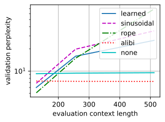
def eval_ppl(model, data):
    @nnx.jit
    def batch_loss(model, X, Y):
        logits = model(X)
        return optax.softmax_cross_entropy_with_integer_labels(
            logits.reshape(-1, logits.shape[-1]), Y.reshape(-1)).mean()
    losses = [float(batch_loss(model, jnp.asarray(X), jnp.asarray(Y)))
              for X, Y in data.val_dataloader()]
    return math.exp(sum(losses) / len(losses))

contexts = (128, 256, 512)
ppls = {pos: [] for pos in schemes}
for ctx in contexts:
    eval_data = d2l.TimeMachine(batch_size=16, num_steps=ctx,
                                tokenization='char', num_train=100000,
                                num_val=3000)
    for pos in schemes:
        ppls[pos].append(eval_ppl(models[pos], eval_data))
for pos in schemes:
    print(f'{pos:>10}: ' + '  '.join(f'{p:7.1f}' for p in ppls[pos]))
d2l.plot(list(contexts), [ppls[pos] for pos in schemes],
         'evaluation context length', 'validation perplexity',
         legend=list(schemes), yscale='log',
         fmts=('-', 'm--', 'g-.', 'r:', 'c-'))
learned: 6.2 18.0 31.1
sinusoidal: 7.8 17.4 38.3
rope: 5.1 10.3 37.0
alibi: 7.1 7.1 7.1
none: 9.2 9.4 9.5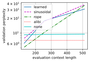
For this fixed seed and training protocol, explicit position information improves perplexity at the training length: RoPE is lowest, followed by the learned table, while sinusoidal embeddings and ALiBi are similar and NoPE is higher. This comparison does not isolate the cause of the differences; for example, describing ALiBi’s result as a consequence of its recency bias would require a separate intervention.
At contexts longer than those seen during training, the learned and sinusoidal absolute schemes deteriorate. The learned table has untrained rows beyond position 128, whereas the sinusoidal table supplies vectors outside the training distribution. RoPE also deteriorates in this run. Although its score depends on relative offset, offsets beyond 127 did not occur during training, so relative parameterization alone does not guarantee length extrapolation. ALiBi and NoPE remain approximately flat in this experiment. Since each curve comes from one seed in each framework, these observations illustrate the possible behavior of the schemes; they do not establish a stable ranking or an estimate of run-to-run variation.
10.4.4.4 Extending a Trained Model’s Context
At an unseen offset such as 400, RoPE rotates the high-frequency pairs through angles absent from the training data. Because these angles vary continuously, they can be rescaled so that the deployed range maps into the trained range. Evaluating at length \(4L\) with every angle multiplied by \(1/4\) makes position \(4\delta\) look like the familiar \(\delta\): interpolation instead of extrapolation. This is position interpolation (Chen et al. 2023), which (with a brief fine-tune) extended Llama from 2k to 32k context; YaRN (Peng et al. 2024) refines it by rescaling the fast, position-discriminating frequencies differently from the slow, content-carrying ones. Many long-context RoPE models use schemes from this family. Note that the recipe has two halves: rescaling and a brief fine-tune at the scaled angles. Exercise 13 walks through both halves on our character model; in our runs, rescaling alone increases perplexity because compressing the angle range makes neighboring characters less distinguishable in the high-frequency pairs. Rescaling followed by a few hundred fine-tuning steps recovers most of the lost performance.
10.4.5 Summary
Unmasked attention is permutation equivariant. Absolute position embeddings break this symmetry by adding a position-dependent vector to each token; sinusoidal embeddings define the vectors analytically, while learned tables are learned only at positions used during training. RoPE rotates query and key feature pairs so their inner product depends on relative offset. ALiBi adds a per-head linear distance penalty, and NoPE uses only the positional asymmetry supplied by the causal mask. In the fixed-seed character-model experiment, RoPE has the lowest perplexity at the training length, while both absolute encodings and RoPE degrade at four times that length. ALiBi and NoPE are approximately stable in that run. Position interpolation and YaRN rescale RoPE frequencies to map longer contexts into the trained range.
10.4.6 Exercises
[code] Causal masks and symmetry. The proposition of Section 10.4.1 assumes that no mask is present. Repeat its numerical check on
d2l.MultiHeadAttentionwith the per-query valid lengths \((1, 2, \ldots, 8)\), which implement the causal mask of Section 10.2.- Measure the maximum output difference as in the unmasked check.
- Identify the step of the proof that fails. Which matrix is not conjugated by \(\boldsymbol{\Pi}\) once the mask is present?
- Show that the output at position \(t\) is unchanged by any permutation that fixes \(t\) and only rearranges the positions before it. What is then the only positional information that the first layer of a NoPE model can carry?
Biases that keep the symmetry. ● Suppose that a fixed matrix \(\mathbf{B} \in \mathbb{R}^{n \times n}\) is added to the score matrix \(\mathbf{S}\) of the proof before the softmax, so that the layer Equation 10.4.1 computes \(\mathrm{softmax}(\mathbf{S} + \mathbf{B})\, \mathbf{X}\mathbf{W}_v\).
- Show that the proposition still holds for every permutation matrix \(\boldsymbol{\Pi}\) with \(\boldsymbol{\Pi}^\top \mathbf{B} \boldsymbol{\Pi} = \mathbf{B}\).
- Find all matrices \(\mathbf{B}\) that satisfy this condition for every permutation, and describe how each of them changes the attention weights.
- Without the causal mask, the ALiBi bias of Equation 10.4.6 extends symmetrically to \(B_{ij} = -m_h\,|i - j|\). Determine the permutations that preserve this matrix, and state what the result implies for an unmasked layer that receives this bias and no other positional signal. Explain why the causal ALiBi of Equation 10.4.6 does not share this symmetry.
Distinct positions, distinct codes. Let \(\mathbf{p}_i\) be row \(i\) of the sinusoidal table Equation 10.4.2 of width \(d\), with the frequencies \(\omega_j = 1/10000^{2j/d}\) of
- Show that \[\mathbf{p}_i^\top \mathbf{p}_{i+\delta} = \sum_{j=0}^{d/2-1} \cos(\delta\,\omega_j),\] derive \(\|\mathbf{p}_i - \mathbf{p}_{i+\delta}\|^2\) from it, and conclude that both quantities depend on the offset \(\delta\) alone.
- Conclude that \(\mathbf{p}_i = \mathbf{p}_{i'}\) only if \((i - i')\,\omega_j\) is a multiple of \(2\pi\) for every \(j\), and that no two distinct integer positions share a row, whatever the value of
max_len. - The fastest pair has period \(2\pi\), so it nearly repeats at integer offsets close to multiples of \(2\pi\). Find the offset \(\delta < 512\) at which its angle comes closest to a multiple of \(2\pi\), and give the residual angle.
- For \(d = 32\), evaluate \(\|\mathbf{p}_i - \mathbf{p}_{i+\delta}\|\) at this offset and at \(\delta = 1\), and find the offset between \(1\) and \(511\) at which the distance is smallest. Which pairs keep the two positions of the near repeat apart? Relate the answer to the binary counting of Section 10.4.2.1.
[code] Untrained rows. The table
pos_embofmodels['learned']hasmax_len = 512rows, of which training at context 128 used only the first 128.- Explain why rows 128 to 511 of the trained table are bitwise equal to those of a freshly constructed
TinyCharLMwithpos='learned'and the seed of Section 10.4.4.3, and check the claim. By what factor would decoupled weight decay with coefficient \(0.1\) at the learning rate \(10^{-3}\) have shrunk these rows over the 3000 training steps? - Compute the cosine similarities between all 512 rows of the trained table and display them with
d2l.show_heatmaps. Describe the three blocks of the result: trained rows against trained rows, untrained against untrained, and trained against untrained. - By problem 3, the dot products of the sinusoidal rows depend only on \(i - j\), so the sinusoidal similarity matrix is constant along each diagonal \(i - j = \textrm{const}\). For the trained rows 0 to 127, compute the standard deviation of the cosine similarities along each diagonal and average it over the diagonals. Compare the average with the standard deviation of the diagonal means across diagonals, and decide whether training produced a code whose similarities are approximately invariant to shifts.
- Explain why rows 128 to 511 of the trained table are bitwise equal to those of a freshly constructed
[code] Amplitude of the sinusoidal table.
TinyCharLMadds the sinusoidal table at full amplitude, while the token embeddings are initialized with standard deviation \(0.02\).- Compute the root-mean-square entry of the table over the first 128 positions and its ratio to \(0.02\). Which of the two signals dominates the input of the first block at initialization?
- Two outcomes are possible when the table is scaled by \(0.02\) instead. The model may use position as well as before, because the projections can amplify a small but structured signal, or it may behave like the
'none'model. State which perplexity pattern at 128 and at 512 distinguishes the two outcomes. - Retrain the
'sinusoidal'variant with the scaled table, evaluate at all three context lengths, and decide.
Additive codes in the score. With the additive encoding of Section 10.4.2.1, a first-layer head of Equation 10.4.1 scores the inputs at positions \(i\) and \(j\) as
\[\mathrm{score}_{ij} = (\mathbf{x}_i + \mathbf{p}_i)^\top \mathbf{A}\, (\mathbf{x}_j + \mathbf{p}_j), \qquad \mathbf{A} = \mathbf{W}_q \mathbf{W}_k^\top / \sqrt{d}. \tag{10.4.7}\]
- Expand the score into its four terms, and state which of them depend on \(i\), which on \(j\), and which on both.
- Let \(\mathbf{J}\) be the rotation of the plane by \(\pi/2\). Using Equation 10.4.3, show that the position–position term \(\mathbf{p}_i^\top \mathbf{A}\, \mathbf{p}_j\) depends only on \(j - i\) when \(\mathbf{A}\) is block diagonal with \(2 \times 2\) blocks \(a_m \mathbf{I} + b_m \mathbf{J}\), one per frequency pair. Problem 3 treats \(\mathbf{A} = \mathbf{I}\). Then show that a single nonzero entry of \(\mathbf{A}\) that couples two different frequency pairs destroys this property.
- Determine when the content–position term \(\mathbf{x}_i^\top \mathbf{A}\, \mathbf{p}_j\) is unchanged for every shift of \(j\). Use the answer to explain the score change of the additive encoding in the shift test of Section 10.4.3, and why RoPE has no content–position term.
Offset preference in RoPE. ● Split a query \(\mathbf{q}\) and a key \(\mathbf{k}\) into the \(d/2\) two-dimensional pairs \(\mathbf{q}^{(m)}, \mathbf{k}^{(m)} \in \mathbb{R}^2\) on which Equation 10.4.5 acts, and let \(\delta = j - i\) be the offset of the key position \(j\) from the query position \(i\).
- Show that the RoPE score Equation 10.4.4 equals \[\sum_{m=0}^{d/2-1} \|\mathbf{q}^{(m)}\|\, \|\mathbf{k}^{(m)}\| \cos(\delta\,\omega_m - \varphi_m), \tag{10.4.8}\] where \(\varphi_m\) is the angle from \(\mathbf{k}^{(m)}\) to \(\mathbf{q}^{(m)}\).
- Choose the angles \(\varphi_m\) so that every pair contributes its maximum at the offset \(\delta = -1\), the previous token. With all products \(\|\mathbf{q}^{(m)}\|\, \|\mathbf{k}^{(m)}\|\) equal to \(c\), show that the score, as a function of \(\delta\), is \(c\) times a shifted copy of the dot product \(\mathbf{p}_i^\top \mathbf{p}_{i+\delta}\) of problem 3 for a sinusoidal table of width \(d\).
- Take \(d = 32\) and the query at position 127, which attends to the offsets \(\delta = -127, \ldots, 0\). Let the attention logits equal these scores, with the factor \(1/\sqrt{d}\) absorbed into \(c\). Find the \(c\) at which the offset \(-1\) receives half of the softmax weight, and identify the offsets that compete most with it. Which pairs set the gap between the score at \(-1\) and the scores at its neighbors?
[code] RoPE at explicit positions.
ropeassumes that the rows of its input sit at consecutive positions starting atoffset. Re-implement it as a class that is constructed with the frequency basebase, the query widthd_k, andmax_seq_len, precomputes the cosine and sine tables once, and applies the rotation at the integer positions given by atoken_positionsarray of arbitrary leading batch shape.- Verify that the class reproduces
rope(x)on the positions \(0, \ldots, T-1\) andrope(x, offset)on the positions \(\textrm{offset}, \ldots, \textrm{offset} + T - 1\). - A packed row of Section 10.2 concatenates several documents and masks attention between them. Explain why restarting the positions at \(0\) for each document leaves every unmasked RoPE score unchanged.
- A row instead holds a shared prefix of 8 tokens followed by two alternative continuations A and B of 4 tokens each, as when several candidate continuations are scored in one pass. Give the tokens of both A and B the positions 8 to 11, and mask attention between A and B. Verify that the scores of the queries of B against the prefix and against B equal those of the row formed by the prefix and B alone, and explain why the consecutive positions \(0, \ldots, 15\), which are all that one call of
ropeon the 16-token row can express, do not give this result.
Adapted from Stanford CS336, Assignment 1, Problem (rope).
- Verify that the class reproduces
[code] Attention by distance. For one head of
TinyCharLM, the distance profile is the average attention weight on the key at distance \(r = i - j\) from the query, taken over queries and validation sequences.TinyCharLM.attention_weightsreturns the maps from which it is computed.- At context 128, compute the profiles of the eight heads of
models['rope']and ofmodels['none']over the queries at positions 64 to 127. Summarize each head by its mass on \(r \leq 3\) and by its mean row entropy. Which heads of the RoPE model attend locally, and what do the heads of the NoPE model do instead? - Relate the difference to the perplexity gap between the two models at the training length. What does a character model gain from heads that attend to the immediately preceding positions?
- At context 128, compute the profiles of the eight heads of
[code] Position through the mask. ● NoPE receives positional information only through the causal mask. Measure how much of it reaches the representation.
- Collect the final residual vector \(\mathbf{h}_i\) that
TinyCharLMpasses to its output head, at every position of the length-128 validation sequences, formodels['none']and formodels['rope']; the loop inattention_weightsshows where to read it. - Train a linear probe that predicts the position index \(i\) from \(\mathbf{h}_i\) as a 128-way classification, and report its held-out accuracy for both models against the chance level \(1/128\). Which positions are predicted best?
- Repeat the probe on an untrained
TinyCharLMwithpos='none'. Which positions can it identify, and how does the variance of an average of \(i + 1\) random vectors explain the result?
- Collect the final residual vector \(\mathbf{h}_i\) that
[code] Where extrapolation fails. The perplexities of Section 10.4.4.3 at context 512 average the loss over all positions of each sequence.
- Show that in each of the five models the logits at positions 0 to 127 of a length-512 sequence agree, up to floating-point round-off, with those computed from its first 128 tokens alone. What does this imply about the positions at which the perplexity changes between context 128 and context 512?
- Compute the validation loss at every position of the length-512 sequences for the five models, average it over windows of 16 positions, and plot it against position. For each scheme, where does the curve leave the level it holds below position 128, and does the loss jump at position 128 or grow gradually?
- Restrict every query of
models['rope']to the 128 most recent keys, itself included, by adding a band constraint to the causal mask in_attend, and repeat the measurement. Compare the windowed curve beyond position 128 with the unwindowed curve below it. Do offsets beyond 127 account for the degradation of RoPE at context 512? - ALiBi stays approximately flat at context 512. For the query at position 511 and equal content scores for all keys, compute the fraction of the weight that each of the slopes of Equation 10.4.6 with \(H = 4\) leaves on the distances \(i - j \geq 128\), none of which occurred in training. Measure the same fraction for the eight heads of
models['alibi']at context 512, and decide whether the stability of ALiBi at that length comes from never attending beyond the training range.
[code] The RoPE base. ● In Equation 10.4.5 the frequencies are \(\omega_m = 10000^{-2m/d}\), and the constant \(10000\) is a choice.
- For the per-head width 32 of
TinyCharLM, compute the periods \(2\pi/\omega_m\) of the 16 pairs for the bases \(100\), \(10^4\), and \(10^6\), and count the pairs that complete at least one full rotation within 128 positions. Which period does not depend on the base? - Add a constructor argument
rope_base, with default \(10^4\), toTinyCharLM, use it in_rope, and retrain the'rope'variant with bases \(100\) and \(10^6\). Use two seeds for each base and one further seed for base \(10^4\), so that differences between bases can be compared with the variation across seeds. Compare perplexity at 128, 256, and 512. - Explain from the counts why the base is expected to matter more at length 512 than at 128, and check the expectation against your results.
- For the per-head width 32 of
[extended] Position interpolation. ● Section 10.4.4.4 describes the effect of rescaling the RoPE angles by \(128/512\) on
models['rope']at context 512, alone and followed by a brief fine-tune, without giving numbers. Fill them in.- Show that a pair that completes a full rotation within the training offsets 0 to 127 has already met, to within \(\omega_m/2\) modulo \(2\pi\), every angle that a longer offset produces. Using the counts of problem 12 for base \(10^4\), determine which pairs a uniform rescaling by \(128/512\) compresses although they did not need it. Compute the gap of problem 7 between the score at offset \(-1\) and the scores at its neighbors for \(d = 32\), before and after the rescaling, and for the rescaling of only the pairs whose period exceeds 128 positions.
- Redefine the method
TinyCharLM._ropeso that it multiplies the angle of each pair by the entry of a model attributerope_scale(all ones when the attribute is absent). Set every entry to \(128/512\) on the trainedmodels['rope'], evaluate it at context 512, and compare with its unscaled perplexity at 512 and with the ALiBi result of Section 10.4.4.3. - Rescale only the pairs whose period exceeds 128 positions and evaluate again without fine-tuning. This is a simplified form of the selective rescaling of YaRN (Peng et al. 2024).
- Fine-tune for a few hundred steps at context 512 with each of the two rescalings, re-evaluate at 128, 256, and 512, and compare with the ALiBi result.