%matplotlib inline
from d2l import torch as d2l
import math
import torch
from torch import nn17.11 Discrete Diffusion
Every diffusion model in this chapter has corrupted continuous data with Gaussian noise. The choice is natural for images and meaningless for text: a token is one element of a finite vocabulary, and adding a real number to its index produces nothing. The same holds for code, for molecules written as strings, and for images once their pixel values are read as categories. This section carries the diffusion construction to such data. What a diffusion model offers for tokens parallels what it offers for continuous data: a likelihood bound to train and evaluate, generation that fills in many positions in parallel and conditions on context on both sides of a gap, and a controllable trade-off between the number of steps and the quality of the samples. The forward process becomes a Markov chain on a finite state space, with transitions given by matrices instead of Gaussian kernels. The variational bound of Section 17.7 goes through unchanged, because its derivation never used the form of the noise. For the corruption that has proved most useful, replacing tokens by a mask symbol, the bound collapses to a cross-entropy on the masked positions with a step-dependent weight. The result is the masked diffusion model behind the diffusion language models of recent years. As before, the running example, quantized to a grid, provides a test with a known answer, and Fashion-MNIST, binarized, provides images.
%matplotlib inline
from d2l import jax as d2l
import math
import jax
from jax import numpy as jnp
from jax.scipy.special import xlogy
from jax.scipy.stats import norm
from flax import nnx
import optax
17.11.1 Corrupting Tokens
17.11.1.1 Transition Matrices
Let a token take one of \(K\) values, written as a one-hot row vector \(\mathbf{x} \in \{0, 1\}^K\). A Markov chain on this space is specified by transition matrices \(Q_t \in [0, 1]^{K \times K}\) whose rows sum to one: \([Q_t]_{ij}\) is the probability of moving from value \(i\) to value \(j\) at step \(t\), so that
\[ q(\mathbf{x}_t \mid \mathbf{x}_{t-1}) = \mathrm{Cat}(\mathbf{x}_t;\ \mathbf{x}_{t-1} Q_t), \tag{17.11.1}\]
where \(\mathrm{Cat}(\mathbf{x}; \mathbf{p})\) denotes the categorical distribution with probability vector \(\mathbf{p}\), and the row vector \(\mathbf{x}_{t-1} Q_t\) is the row of \(Q_t\) selected by the current value. This is the framework of Austin et al. (2021); the binary case appears already in Sohl-Dickstein et al. (2015) and the uniform kernel below in Hoogeboom et al. (2021) . A sequence of \(L\) tokens is corrupted by applying the chain to every position independently. The two properties of the Gaussian chain that Section 17.7 relied on both hold here. The marginal after \(t\) steps is given by a product of matrices,
\[ q(\mathbf{x}_t \mid \mathbf{x}_0) = \mathrm{Cat}(\mathbf{x}_t;\ \mathbf{x}_0 \bar{Q}_t), \qquad \bar{Q}_t = Q_1 Q_2 \cdots Q_t, \tag{17.11.2}\]
by induction on \(t\), since composing two Markov transitions multiplies their matrices. The posterior of one step given both endpoints follows from Bayes’ rule and the Markov property,
\[ q(\mathbf{x}_{t-1} \mid \mathbf{x}_t, \mathbf{x}_0) = \frac{q(\mathbf{x}_t \mid \mathbf{x}_{t-1})\, q(\mathbf{x}_{t-1} \mid \mathbf{x}_0)}{q(\mathbf{x}_t \mid \mathbf{x}_0)} = \mathrm{Cat}\!\left(\mathbf{x}_{t-1};\ \frac{\mathbf{x}_t Q_t^\top \odot \mathbf{x}_0 \bar{Q}_{t-1}}{\mathbf{x}_0 \bar{Q}_t \mathbf{x}_t^\top}\right), \tag{17.11.3}\]
where \(\odot\) is the elementwise product. The vector \(\mathbf{x}_t Q_t^\top\) lists, for every possible predecessor, the probability of reaching the observed \(\mathbf{x}_t\) from it; \(\mathbf{x}_0 \bar{Q}_{t-1}\) lists the probability of each predecessor given the start; and the denominator normalizes. Both formulas hold for any sequence of matrices, and the second is what the variational bound requires.
17.11.1.2 Two Kernels
The matrices are chosen so that the products in Equation 17.11.2 have a closed form and the chain forgets its start. The uniform kernel resamples a token uniformly from the vocabulary with probability \(\beta_t\) and keeps it otherwise,
\[ Q_t = (1 - \beta_t)\, I + \beta_t\, \tfrac{1}{K} \mathbf{1}\mathbf{1}^\top, \]
where \(\mathbf{1}\) is the all-ones vector; its stationary distribution is uniform over the vocabulary, the counterpart of the standard Gaussian. The absorbing kernel enlarges the vocabulary by one value, the mask \([\textrm{M}]\), and moves each token there with probability \(\beta_t\); a masked token stays masked:
\[ Q_t = (1 - \beta_t)\, I + \beta_t\, \mathbf{1} \mathbf{e}_{\textrm{M}}^\top, \tag{17.11.4}\]
with \(\mathbf{e}_{\textrm{M}}\) the one-hot vector of the mask. For both kernels the products collapse. Write \(\bar{\alpha}_t = \prod_{s \leq t} (1 - \beta_s)\) as in Section 17.7, and let \(P\) stand for \(\tfrac{1}{K}\mathbf{1}\mathbf{1}^\top\) or for \(\mathbf{1}\mathbf{e}_{\textrm{M}}^\top\); in both cases \(P^2 = P\), so \((aI + bP)(cI + dP) = ac\, I + (ad + bc + bd)\, P\), and when \(a + b = c + d = 1\) the second coefficient equals \(1 - ac\). The coefficient of \(I\) therefore multiplies along the chain and
\[ \bar{Q}_t = \bar{\alpha}_t\, I + (1 - \bar{\alpha}_t)\, \tfrac{1}{K}\mathbf{1}\mathbf{1}^\top \quad\textrm{(uniform)}, \qquad \bar{Q}_t = \bar{\alpha}_t\, I + (1 - \bar{\alpha}_t)\, \mathbf{1}\mathbf{e}_{\textrm{M}}^\top \quad\textrm{(absorbing)}. \tag{17.11.5}\]
In words, after \(t\) steps of the absorbing chain a token still carries its original value with probability \(\bar{\alpha}_t\) and has been replaced by the mask with probability \(1 - \bar{\alpha}_t\), independently across positions. The chain never confuses one token with another; it only erases. A schedule with \(\bar{\alpha}_T = 0\) ends at the fully masked sequence, a state that carries no information about the data, as the Gaussian chain ended at pure noise. Figure 17.11.1 shows the two directions.
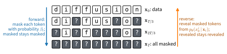
The rest of the section uses the absorbing kernel. It is the choice behind the diffusion language models cited below; Austin et al. (2021) already found that it gave the best likelihoods on text among the kernels they compared, and its posterior is the simplest, as the next subsection shows.
17.11.2 The Variational Bound for Masked Tokens
17.11.2.1 The Same Bound, a Different Target
The reverse model is again a Markov chain \(p_{\boldsymbol{\theta}}(\mathbf{x}_{t-1} \mid \mathbf{x}_t)\), started from the all-mask sequence, and the derivation of Equation 17.7.6 applies verbatim, because it used only the Markov property and Bayes’ rule:
\[ L_{\textrm{VLB}} = \mathrm{KL}\big(q(\mathbf{x}_T \mid \mathbf{x}_0)\, \|\, p(\mathbf{x}_T)\big) + \sum_{t=2}^{T} \mathbb{E}_q\Big[\mathrm{KL}\big(q(\mathbf{x}_{t-1} \mid \mathbf{x}_t, \mathbf{x}_0)\, \|\, p_{\boldsymbol{\theta}}(\mathbf{x}_{t-1} \mid \mathbf{x}_t)\big)\Big] + \mathbb{E}_q\big[-\log p_{\boldsymbol{\theta}}(\mathbf{x}_0 \mid \mathbf{x}_1)\big]. \]
Every divergence is now between categorical distributions and is a finite sum. What changes is the parameterization. In the Gaussian case the network predicted the noise; here the natural target is the clean token itself. Following Austin et al. (2021), the network outputs, for each position \(i\), a distribution \(p_{\boldsymbol{\theta}}(\mathbf{x}_0^i \mid \mathbf{x}_t)\) over the \(K\) clean values given the whole corrupted sequence, and the reverse transition averages the true posterior over this prediction,
\[ p_{\boldsymbol{\theta}}(\mathbf{x}_{t-1} \mid \mathbf{x}_t) = \sum_{\hat{\mathbf{x}}_0} q(\mathbf{x}_{t-1} \mid \mathbf{x}_t, \hat{\mathbf{x}}_0)\, p_{\boldsymbol{\theta}}(\hat{\mathbf{x}}_0 \mid \mathbf{x}_t), \tag{17.11.6}\]
position by position, with the prediction at an unmasked position taken to be the observed token. This is the discrete counterpart of predicting the clean point and inserting it into the Gaussian posterior Equation 17.7.7. Austin et al. (2021) write the average over the joint \(q(\mathbf{x}_{t-1}, \mathbf{x}_t \mid \hat{\mathbf{x}}_0)\) and renormalize, which reweights the candidates by \(q(\mathbf{x}_t \mid \hat{\mathbf{x}}_0)\); for the absorbing kernel that weight is the same for every candidate at a masked position, so the two forms agree, whereas for the uniform kernel they differ (Exercise 1).
17.11.2.2 The Posterior of the Absorbing Chain
Proposition (posterior of the absorbing chain). Under the absorbing kernel with \(\beta_1 > 0\), so that \(\bar{\alpha}_t < 1\) for every \(t \geq 1\), consider one position with clean value \(\mathbf{x}_0 \neq [\textrm{M}]\). If \(\mathbf{x}_t = \mathbf{x}_0\), then \(\mathbf{x}_{t-1} = \mathbf{x}_0\) with probability one. If \(\mathbf{x}_t = [\textrm{M}]\), then
\[ q(\mathbf{x}_{t-1} = \mathbf{x}_0 \mid \mathbf{x}_t = [\textrm{M}], \mathbf{x}_0) = \frac{\bar{\alpha}_{t-1} - \bar{\alpha}_t}{1 - \bar{\alpha}_t}, \qquad q(\mathbf{x}_{t-1} = [\textrm{M}] \mid \mathbf{x}_t = [\textrm{M}], \mathbf{x}_0) = \frac{1 - \bar{\alpha}_{t-1}}{1 - \bar{\alpha}_t}, \tag{17.11.7}\]
and no other value has positive probability.
Proof. Evaluate Equation 17.11.3 with Equation 17.11.4 and 1. The vector \(\mathbf{x}_0 \bar{Q}_{t-1}\) puts mass \(\bar{\alpha}_{t-1}\) on \(\mathbf{x}_0\) and \(1 - \bar{\alpha}_{t-1}\) on the mask, so only these two predecessors are possible. If \(\mathbf{x}_t = \mathbf{x}_0\), the vector \(\mathbf{x}_t Q_t^\top\) has the entry \(1 - \beta_t\) at \(\mathbf{x}_0\) and the entry \(0\) at the mask, because a mask never returns to a token, and the posterior is a point mass. If \(\mathbf{x}_t = [\textrm{M}]\), the entries are \(\beta_t\) at \(\mathbf{x}_0\) and \(1\) at the mask, so the unnormalized posterior is \(\bar{\alpha}_{t-1}\beta_t\) on \(\mathbf{x}_0\) and \(1 - \bar{\alpha}_{t-1}\) on the mask. Their sum, \(1 - \bar{\alpha}_{t-1}(1 - \beta_t) = 1 - \bar{\alpha}_t\), is the denominator \(q(\mathbf{x}_t = [\textrm{M}] \mid \mathbf{x}_0)\), and \(\bar{\alpha}_{t-1}\beta_t = \bar{\alpha}_{t-1} - \bar{\alpha}_t\). \(\blacksquare\)
One step back, a masked token either stays masked or reverts to its clean value, and an unmasked token is left alone. The reverse model Equation 17.11.6 therefore takes a concrete form. It keeps every unmasked position, and at each masked position it independently either keeps the mask, with probability \((1 - \bar{\alpha}_{t-1}) / (1 - \bar{\alpha}_t)\), or replaces it by a draw from \(p_{\boldsymbol{\theta}}(\mathbf{x}_0^i \mid \mathbf{x}_t)\).
17.11.2.3 A Weighted Cross-Entropy
Proposition (masked diffusion bound). For the absorbing kernel with \(\bar{\alpha}_0 = 1\), \(\bar{\alpha}_t < 1\) for \(t \geq 1\), and \(\bar{\alpha}_T = 0\), and the reverse model just described,
\[ L_{\textrm{VLB}} = \sum_{t=1}^{T} \frac{\bar{\alpha}_{t-1} - \bar{\alpha}_t}{1 - \bar{\alpha}_t}\; \mathbb{E}_{q(\mathbf{x}_t \mid \mathbf{x}_0)}\Big[ \sum_{i \,:\, \mathbf{x}_t^i = [\textrm{M}]} -\log p_{\boldsymbol{\theta}}(\mathbf{x}_0^i \mid \mathbf{x}_t) \Big]. \tag{17.11.8}\]
Proof. The prior term vanishes: \(\bar{\alpha}_T = 0\) makes \(q(\mathbf{x}_T \mid \mathbf{x}_0)\) the point mass on the all-mask sequence, which is also \(p(\mathbf{x}_T)\). Both \(q(\mathbf{x}_{t-1} \mid \mathbf{x}_t, \mathbf{x}_0)\) and \(p_{\boldsymbol{\theta}}(\mathbf{x}_{t-1} \mid \mathbf{x}_t)\) factorize over positions, so each divergence is a sum of per-position divergences. At an unmasked position both distributions are the same point mass and the divergence is zero. At a masked position write \(w_t = (\bar{\alpha}_{t-1} - \bar{\alpha}_t) / (1 - \bar{\alpha}_t)\). The true posterior puts \(1 - w_t\) on the mask and \(w_t\) on \(\mathbf{x}_0^i\); the model puts \(1 - w_t\) on the mask and \(w_t\, p_{\boldsymbol{\theta}}(\cdot \mid \mathbf{x}_t)\) on the tokens; hence
\[ \mathrm{KL} = (1 - w_t) \log \frac{1 - w_t}{1 - w_t} + w_t \log \frac{w_t}{w_t\, p_{\boldsymbol{\theta}}(\mathbf{x}_0^i \mid \mathbf{x}_t)} = -w_t \log p_{\boldsymbol{\theta}}(\mathbf{x}_0^i \mid \mathbf{x}_t). \]
This accounts for \(t = 2, \ldots, T\). The reconstruction term is \(\mathbb{E}[-\log p_{\boldsymbol{\theta}}(\mathbf{x}_0 \mid \mathbf{x}_1)]\); since \(w_1 = (1 - \bar{\alpha}_1)/(1 - \bar{\alpha}_1) = 1\), the model replaces every position masked at step \(1\) by a draw from \(p_{\boldsymbol{\theta}}(\cdot \mid \mathbf{x}_1)\) and copies the rest, so this term equals the sum of \(-\log p_{\boldsymbol{\theta}}(\mathbf{x}_0^i \mid \mathbf{x}_1)\) over the masked positions, which is the \(t = 1\) term of the sum. \(\blacksquare\)
The bound Equation 17.11.8 is a cross-entropy on the masked positions of a partially masked sequence, weighted by a factor that depends on the step, and it is an upper bound on the negative log-likelihood \(-\log p_{\boldsymbol{\theta}}(\mathbf{x}_0)\): unlike the adversarial models of Chapter 16, the model assigns every sequence a probability that can be bounded and compared. Austin et al. (2021) already noted that the bound of the absorbing chain reduces to a reweighted masked-language-model loss, but trained the general bound with an added cross-entropy term; the masked diffusion language models of Sahoo et al. (2024) and Shi et al. (2024) take Equation 17.11.8 itself, and its continuous-time limit, as the objective. Under the linear schedule \(\bar{\alpha}_t = 1 - t/T\), a fraction \(t/T\) of the tokens is masked at step \(t\) and the weight is \(w_t = (1/T)/(t/T) = 1/t\): an error at a heavily masked sequence is charged less than the same error at a lightly masked one. Since the number of masked positions grows in proportion to \(t\), every step carries the same expected weighted count of masked positions, \(L/T\) for a sequence of \(L\) tokens; the steps differ only in how hard their masked tokens are to predict. The sum is also a Riemann sum. Letting \(T \to \infty\) with \(\bar{\alpha}_t = \bar{\alpha}(t/T)\) for a decreasing function \(\bar{\alpha}\) on \([0, 1]\), the bound tends to \(\int_0^1 \frac{-\bar{\alpha}'(\tau)}{1 - \bar{\alpha}(\tau)}\, \mathbb{E}\big[\sum_{\textrm{masked}} -\log p_{\boldsymbol{\theta}}\big]\, d\tau\), and the substitution \(u = 1 - \bar{\alpha}(\tau)\), the masking probability, turns this into \(\int_0^1 \frac{1}{u}\, \mathbb{E}_u[\cdots]\, du\), where \(\mathbb{E}_u\) masks each token with probability \(u\). If the network is told the masking probability rather than the raw step, the limiting bound does not depend on the schedule at all, only on how well the network predicts masked tokens at every masking level. This is the discrete analogue of the schedule invariance that Kingma et al. (2021) established for Gaussian diffusion, and both papers above note it.
17.11.3 Sampling by Unmasking
Generation runs the reverse model from the all-mask sequence. At step \(t\), one forward pass yields \(p_{\boldsymbol{\theta}}(\cdot \mid \mathbf{x}_t)\) at every masked position; each masked position draws a candidate token and accepts it with probability \(w_t\), and accepted tokens are never revised. Under the linear schedule \(w_t = 1/t\), so about a fraction \(1/t\) of the tokens still masked at step \(t\) is revealed; since about \(t/T\) of the \(L\) tokens are still masked, roughly \(L/T\) tokens are revealed per step, a constant rate. Fewer steps are available as they were for DDIM in Section 17.9: choose levels \(T = t_0 > t_1 > \cdots > t_S = 0\). The coarser chain has the same marginals 1, the computation of the proposition applies to it unchanged, and a jump from \(t_k\) to \(t_{k+1}\) reveals each masked token with probability \((\bar{\alpha}_{t_{k+1}} - \bar{\alpha}_{t_k}) / (1 - \bar{\alpha}_{t_k})\). With \(S = 1\) everything is revealed at once from the prediction at the all-mask input.
Fewer steps have a specific cost. The tokens revealed in the same step are drawn independently from their own predicted distributions, because the network’s prediction is a product over positions; tokens revealed in different steps are drawn one after another, each conditioned on the ones already revealed. A pair of tokens revealed together therefore follows the product of two marginals rather than their joint distribution. The running example, quantized to a pair of tokens as the experiments below describe, makes this exact. It has two tokens, and under the linear schedule the pattern of masks at level \(t_k\) has each token masked independently with probability \(t_k / T\), while the jump to \(t_{k+1}\) reveals a masked token with probability \((t_k - t_{k+1}) / t_k\); both tokens are revealed in that jump with probability \((t_k / T)^2 \cdot ((t_k - t_{k+1}) / t_k)^2 = 1/S^2\) for equally spaced levels, and summing over the \(S\) jumps gives \(1/S\). With an exact network, one whose prediction at each masked position is the true conditional distribution of that token given the unmasked ones, the sampler thus produces the mixture \((1 - 1/S)\, p + (1/S)\, p^1 \otimes p^2\) of the true joint and the product of its marginals, whose total variation distance from \(p\) is \(\mathrm{TV}(p^1 \otimes p^2, p) / S\). The experiments below measure this.
The sampler also places masked diffusion among older models. Trained at a single masking level, Equation 17.11.8 is the masked language modeling objective of BERT (Devlin et al. 2018), up to BERT’s replacement of some masks by random or unchanged tokens, so a masked language model is a one-step discrete diffusion model, as Austin et al. (2021) point out. Reveal exactly one token per step in a random order and the sampler is an order-agnostic autoregressive model (Uria et al. 2014); fix the order to left-to-right and it is an ordinary autoregressive language model, whose conditionals are the network’s predictions \(p_{\boldsymbol{\theta}}(\mathbf{x}_0^i \mid \mathbf{x}_t)\) at inputs in which a prefix is unmasked and the remainder is masked, a correspondence that Austin et al. (2021) also draw. Between these extremes, the number of steps trades sequential computation for the independence error above. The framework has a continuous-time formulation (Campbell et al. 2022) and a score-based one: Lou et al. (2024) learn ratios \(p_t(\mathbf{y}) / p_t(\mathbf{x})\) between neighboring sequences, the discrete counterpart of the score, and train them with a loss that plays the role of score matching. Nie et al. (2025) have since trained a masked diffusion language model with eight billion parameters and report that it is competitive with an autoregressive model of the same size, LLaMA 3 8B, in in-context learning.
17.11.4 Experiments on the Running Example
Quantizing the mixture onto a \(32 \times 32\) grid over \([-5, 5]^2\), with points outside the square assigned to the edge cell nearest to them, turns each sample into a pair of tokens, its row and column indices: a sequence of length two over a vocabulary of \(K = 32\) values. The probability of each cell is the integral of the mixture density over it, the edge cells extending to infinity, and the integral factorizes per component into a product of two one-dimensional Gaussian integrals, so the true table is available exactly, and so is its entropy, the negative log-likelihood that a perfect model attains. Little mass lies outside the square in any case: the nearest mode is five standard deviations from its edge. The cell also prints the bound that an exact network would attain, the entropy plus \(I(X^1; X^2) / T\) with \(I\) the mutual information of the two coordinates, because pairs masked together are predicted independently; Exercise 3 derives it, and the training experiment below uses it as the reference. Two reference quantities accompany the table: the total variation distance between a histogram of \(20{,}000\) true samples and the table, the floor that finite samples impose on every comparison below, and the distance between the product of the two marginals and the table, the error of a model that draws the coordinates independently.
torch.manual_seed(0)
mix = d2l.GaussianMixture(means=[[-2.5, -1.5], [2.5, -1.5], [0.0, 2.5]],
                          weights=[0.5, 0.3, 0.2], std=0.5)
K, T, MASK = 32, 32, 32  # vocabulary size, number of steps, index of the mask
edges = torch.linspace(-5, 5, K + 1)

def quantize(x):  # continuous points to pairs of tokens in {0, ..., K - 1}
    return ((x + 5) / 10 * K).floor().long().clamp(0, K - 1)

data, test = quantize(mix.sample(20000)), quantize(mix.sample(20000))
cdf = torch.distributions.Normal(0.0, 1.0).cdf(
    (edges[None, None, :] - mix.means[:, :, None]) / mix.std)  # (3, 2, K + 1)
cdf[:, :, 0], cdf[:, :, -1] = 0.0, 1.0  # edge cells extend to infinity, as in quantize
per_axis = cdf[:, :, 1:] - cdf[:, :, :-1]  # cell masses of each component, per axis
table = (mix.weights[:, None, None] * per_axis[:, 0, :, None]
         * per_axis[:, 1, None, :]).sum(0)
entropy = -torch.special.xlogy(table, table).sum()

def histogram(z):
    counts = torch.bincount(z[:, 0] * K + z[:, 1], minlength=K * K)
    return counts.reshape(K, K).float() / len(z)

def tv(p, q):  # total variation distance between two tables
    return 0.5 * (p - q).abs().sum()

product = table.sum(1)[:, None] * table.sum(0)[None, :]
marginals = table.sum(1), table.sum(0)
mutual = -sum(torch.special.xlogy(m, m).sum() for m in marginals) - entropy
print(f'entropy of the table: {entropy:.3f} nats; '
      f'bound of an exact network with T = {T}: {entropy + mutual / T:.3f} nats')
print(f'TV(histogram of 20000 true samples, table): {tv(histogram(test), table):.3f}')
print(f'TV(product of the marginals, table): {tv(product, table):.3f}')
entropy of the table: 4.840 nats; bound of an exact network with T = 32: 4.855 nats
TV(histogram of 20000 true samples, table): 0.036
TV(product of the marginals, table): 0.314key = jax.random.PRNGKey(0)
mix = d2l.GaussianMixture(means=[[-2.5, -1.5], [2.5, -1.5], [0.0, 2.5]],
weights=[0.5, 0.3, 0.2], std=0.5)
K, T, MASK = 32, 32, 32 # vocabulary size, number of steps, index of the mask
edges = jnp.linspace(-5, 5, K + 1)
def quantize(x): # continuous points to pairs of tokens in {0, ..., K - 1}
return jnp.clip(jnp.floor((x + 5) / 10 * K), 0, K - 1).astype(jnp.int32)
key, k1, k2 = jax.random.split(key, 3)
data, test = quantize(mix.sample(k1, 20000)), quantize(mix.sample(k2, 20000))
cdf = norm.cdf((edges[None, None, :] - mix.means[:, :, None]) / mix.std) # (3, 2, K + 1)
cdf = cdf.at[:, :, 0].set(0.0).at[:, :, -1].set(1.0) # edge cells extend to infinity
per_axis = cdf[:, :, 1:] - cdf[:, :, :-1] # cell masses of each component, per axis
table = (mix.weights[:, None, None] * per_axis[:, 0, :, None]
* per_axis[:, 1, None, :]).sum(0)
entropy = -xlogy(table, table).sum()
def histogram(z):
counts = jnp.bincount(z[:, 0] * K + z[:, 1], length=K * K)
return counts.reshape(K, K) / len(z)
def tv(p, q): # total variation distance between two tables
return 0.5 * jnp.abs(p - q).sum()
product = table.sum(1)[:, None] * table.sum(0)[None, :]
marginals = table.sum(1), table.sum(0)
mutual = -sum(xlogy(m, m).sum() for m in marginals) - entropy
print(f'entropy of the table: {entropy:.3f} nats; '
f'bound of an exact network with T = {T}: {entropy + mutual / T:.3f} nats')
print(f'TV(histogram of 20000 true samples, table): {tv(histogram(test), table):.3f}')
print(f'TV(product of the marginals, table): {tv(product, table):.3f}')entropy of the table: 4.840 nats; bound of an exact network with T = 32: 4.855 nats
TV(histogram of 20000 true samples, table): 0.041
TV(product of the marginals, table): 0.314The network takes the one-hot encoding of both tokens, with the mask as a thirty-third value, together with the step, and outputs logits over the thirty-two clean values at each position. The training loop draws one step per sequence; the loss function masks each token with probability \(1 - \bar{\alpha}_t\) and evaluates the summand of Equation 17.11.8 at the masked positions, and multiplying by \(T\) makes the single draw of the step an unbiased estimate of the whole sum.
class MaskedMLP(nn.Module):
    """Logits of the clean tokens given a partially masked pair and the step."""
    def __init__(self, hidden=256):
        super().__init__()
        self.net = nn.Sequential(nn.Linear(2 * (K + 1) + 1, hidden), nn.SiLU(),
                                 nn.Linear(hidden, hidden), nn.SiLU(),
                                 nn.Linear(hidden, 2 * K))

    def forward(self, z, t):
        h = torch.cat([nn.functional.one_hot(z, K + 1).float().flatten(1),
                       (t / T)[:, None]], 1)
        return self.net(h).reshape(-1, 2, K)

alpha_bar = 1 - torch.arange(T + 1) / T  # linear schedule; alpha_bar[T] = 0

def masked_loss(model, x0, t):  # one-sample estimate of the bound per sequence, nats
    masked = torch.rand(x0.shape) < (1 - alpha_bar[t])[:, None]
    z = torch.where(masked, MASK, x0)
    logp = torch.log_softmax(model(z, t), -1).gather(-1, x0[..., None])[..., 0]
    weight = (alpha_bar[t - 1] - alpha_bar[t]) / (1 - alpha_bar[t])  # 1 / t
    return (T * weight[:, None] * -logp * masked).sum(1)
class MaskedMLP(nnx.Module):
"""Logits of the clean tokens given a partially masked pair and the step."""
def __init__(self, hidden=256, rngs=None):
self.h1 = nnx.Linear(2 * (K + 1) + 1, hidden, rngs=rngs)
self.h2 = nnx.Linear(hidden, hidden, rngs=rngs)
self.out = nnx.Linear(hidden, 2 * K, rngs=rngs)
def __call__(self, z, t):
h = jnp.concatenate([jax.nn.one_hot(z, K + 1).reshape(len(z), -1),
(t / T)[:, None]], 1)
return self.out(nnx.silu(self.h2(nnx.silu(self.h1(h))))).reshape(-1, 2, K)
alpha_bar = 1 - jnp.arange(T + 1) / T # linear schedule; alpha_bar[T] = 0
def masked_loss(model, x0, t, key): # one-sample estimate of the bound per sequence, nats
masked = jax.random.uniform(key, x0.shape) < (1 - alpha_bar[t])[:, None]
z = jnp.where(masked, MASK, x0)
logp = jnp.take_along_axis(jax.nn.log_softmax(model(z, t), -1),
x0[..., None], -1)[..., 0]
weight = (alpha_bar[t - 1] - alpha_bar[t]) / (1 - alpha_bar[t]) # 1 / t
return (T * weight[:, None] * -logp * masked).sum(1)Because the sequence has two positions, the expectation in Equation 17.11.8 can also be computed exactly: at each step there are three mask patterns with at least one mask, with known probabilities, and the \(1024\) possible pairs are weighted by the true table. The resulting number is the bound averaged over the true distribution, which cannot fall below the entropy of the table. Part of the excess remains even for an exact network: its bound equals the entropy plus \(I(X^1; X^2) / T\), the mutual information of the two coordinates divided by the number of steps (Exercise 3), the cost of predicting the two tokens independently whenever both are masked. No network that predicts the positions independently can go below this floor, whose value the first cell printed. We track the model’s bound during training.
pairs = torch.cartesian_prod(torch.arange(K), torch.arange(K))  # all 1024 pairs
patterns = torch.tensor([[True, False], [False, True], [True, True]])

@torch.no_grad()
def exact_bound(model):  # the bound averaged over the true table, all steps and patterns
    total = 0.0
    for t in range(1, T + 1):
        weight = (alpha_bar[t - 1] - alpha_bar[t]) / (1 - alpha_bar[t])
        for masked in patterns:
            masked = masked.expand(len(pairs), 2)
            z = torch.where(masked, MASK, pairs)
            logp = torch.log_softmax(model(z, torch.full((len(pairs),), t)), -1)
            logp = logp.gather(-1, pairs[..., None])[..., 0]
            n_masked = masked[0].sum()
            prob = (1 - alpha_bar[t]) ** n_masked * alpha_bar[t] ** (2 - n_masked)
            total += prob * weight * (table.flatten() * (-logp * masked).sum(1)).sum()
    return total

torch.manual_seed(1)
model = MaskedMLP()
optimizer = torch.optim.Adam(model.parameters(), lr=1e-3)
for step in range(6000):
    if step == 4000:
        optimizer.param_groups[0]['lr'] = 2e-4
    x0 = data[torch.randint(0, len(data), (512,))]
    t = torch.randint(1, T + 1, (512,))
    loss = masked_loss(model, x0, t).mean()
    optimizer.zero_grad(), loss.backward(), optimizer.step()
    if step % 2000 == 0:
        print(f'step {step:>4}: exact bound {exact_bound(model):.3f} nats')
print(f'final exact bound {exact_bound(model):.3f} nats; entropy {entropy:.3f} nats')
step 0: exact bound 6.918 nats
step 2000: exact bound 4.874 nats
step 4000: exact bound 4.870 nats
final exact bound 4.864 nats; entropy 4.840 natspairs = jnp.stack(jnp.meshgrid(jnp.arange(K), jnp.arange(K), indexing='ij'),
-1).reshape(-1, 2) # all 1024 pairs
patterns = jnp.array([[True, False], [False, True], [True, True]])
def exact_bound(model): # the bound averaged over the true table, all steps and patterns
total = 0.0
for t in range(1, T + 1):
weight = (alpha_bar[t - 1] - alpha_bar[t]) / (1 - alpha_bar[t])
for masked in patterns:
masked = jnp.broadcast_to(masked, pairs.shape)
z = jnp.where(masked, MASK, pairs)
logp = jax.nn.log_softmax(model(z, jnp.full((len(pairs),), t)), -1)
logp = jnp.take_along_axis(logp, pairs[..., None], -1)[..., 0]
n_masked = masked[0].sum()
prob = (1 - alpha_bar[t]) ** n_masked * alpha_bar[t] ** (2 - n_masked)
total += prob * weight * (table.flatten() * (-logp * masked).sum(1)).sum()
return total
@nnx.jit
def masked_step(model, optimizer, x0, t, key):
loss, grads = nnx.value_and_grad(
lambda m: masked_loss(m, x0, t, key).mean())(model)
optimizer.update(model, grads)
return loss
model = MaskedMLP(rngs=nnx.Rngs(1))
schedule = optax.piecewise_constant_schedule(1e-3, {4000: 0.2})
optimizer = nnx.Optimizer(model, optax.adam(schedule), wrt=nnx.Param)
for step in range(6000):
key, k1, k2, k3 = jax.random.split(key, 4)
x0 = data[jax.random.randint(k1, (512,), 0, len(data))]
t = jax.random.randint(k2, (512,), 1, T + 1)
loss = masked_step(model, optimizer, x0, t, k3)
if step % 2000 == 0:
print(f'step {step:>4}: exact bound {exact_bound(model):.3f} nats')
print(f'final exact bound {exact_bound(model):.3f} nats; entropy {entropy:.3f} nats')step 0: exact bound 6.876 nats
step 2000: exact bound 4.875 nats
step 4000: exact bound 4.872 nats
final exact bound 4.864 nats; entropy 4.840 natsThe bound comes within a few hundredths of a nat of the entropy: the model has learned the marginal of each coordinate and its conditional given the other. Most of the remaining gap is the floor printed by the first cell, which an exact network pays as well; the trained network’s own excess over that floor is of the order of a hundredth of a nat. The floor is not all looseness of the bound: the thirty-two-step chain of an exact network reveals both tokens in the same step with probability \(1/32\), so it models \((1 - 1/32)\, p + (1/32)\, p^1 \otimes p^2\) rather than \(p\), as the next experiment shows. The sampler below implements the unmasking described above for any number of steps \(S\), using the levels \(T, T(S-1)/S, \ldots, 0\), and we compare the histogram of \(20{,}000\) samples with the table and with the product of the marginals, next to the prediction \(\mathrm{TV}(p^1 \otimes p^2, p) / S\) for an exact network.
@torch.no_grad()
def unmask(model, n, steps):
    z = torch.full((n, 2), MASK)
    levels = torch.linspace(T, 0, steps + 1).round().long().tolist()
    for t, s in zip(levels[:-1], levels[1:]):
        draw = torch.distributions.Categorical(
            logits=model(z, torch.full((n,), t))).sample()
        reveal = (z == MASK) & (torch.rand(z.shape)
                                < (alpha_bar[s] - alpha_bar[t]) / (1 - alpha_bar[t]))
        z = torch.where(reveal, draw, z)
    return z

torch.manual_seed(2)
samples = {}
print(f'{"steps":>5} {"TV to table":>12} {"predicted":>10} {"TV to product":>14}')
for steps in (32, 8, 2, 1):
    samples[steps] = unmask(model, 20000, steps)
    h = histogram(samples[steps])
    print(f'{steps:>5} {tv(h, table):>12.3f} {tv(product, table) / steps:>10.3f} '
          f'{tv(h, product):>14.3f}')
steps TV to table predicted TV to product
32 0.060 0.010 0.310
8 0.079 0.039 0.282
2 0.175 0.157 0.163
1 0.327 0.314 0.062def unmask(model, key, n, steps):
z = jnp.full((n, 2), MASK)
levels = [round(l) for l in jnp.linspace(T, 0, steps + 1).tolist()]
for t, s in zip(levels[:-1], levels[1:]):
key, k1, k2 = jax.random.split(key, 3)
draw = jax.random.categorical(k1, model(z, jnp.full((n,), t)), axis=-1)
reveal = (z == MASK) & (jax.random.uniform(k2, z.shape)
< (alpha_bar[s] - alpha_bar[t]) / (1 - alpha_bar[t]))
z = jnp.where(reveal, draw, z)
return z
samples = {}
print(f'{"steps":>5} {"TV to table":>12} {"predicted":>10} {"TV to product":>14}')
for steps in (32, 8, 2, 1):
key, subkey = jax.random.split(key)
samples[steps] = unmask(model, subkey, 20000, steps)
h = histogram(samples[steps])
print(f'{steps:>5} {tv(h, table):>12.3f} {tv(product, table) / steps:>10.3f} '
f'{tv(h, product):>14.3f}')steps TV to table predicted TV to product
32 0.061 0.010 0.311
8 0.076 0.039 0.283
2 0.165 0.157 0.171
1 0.302 0.314 0.057With all thirty-two steps the samples are within a few hundredths of the sampling floor. As the number of steps falls, the distance to the table grows as predicted and tracks \(\mathrm{TV}(p^1 \otimes p^2, p) / S\). At thirty-two and eight steps it exceeds the prediction by the model error and the sampling floor; at two and one step it lies within a few hundredths of it, because the systematic error dominates the histogram noise. The distance to the product shrinks correspondingly, and with a single step the samples follow the product of the marginals, as they must, since both coordinates are drawn from the prediction at the all-mask input. The panels show the table and the two extreme histograms; the one-step panel has mass where a row and a column of the mixture cross, at positions where the data has none.
fig, axes = d2l.plt.subplots(1, 3, figsize=(10, 3.4))
for ax, (title, h) in zip(axes, [('true table', table),
                                 ('32 steps', histogram(samples[32])),
                                 ('1 step', histogram(samples[1]))]):
    ax.imshow(h.T, origin='lower', extent=(-5, 5, -5, 5), cmap='Blues')
    ax.set_title(title)
fig.tight_layout()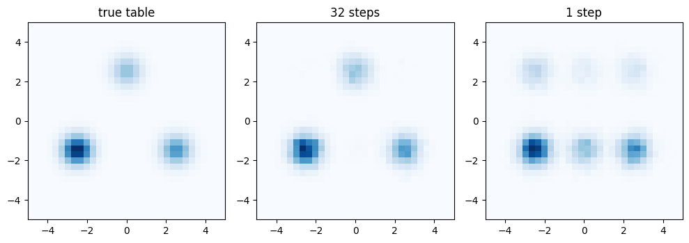
fig, axes = d2l.plt.subplots(1, 3, figsize=(10, 3.4))
for ax, (title, h) in zip(axes, [('true table', table),
                                 ('32 steps', histogram(samples[32])),
                                 ('1 step', histogram(samples[1]))]):
    ax.imshow(h.T, origin='lower', extent=(-5, 5, -5, 5), cmap='Blues')
    ax.set_title(title)
fig.tight_layout()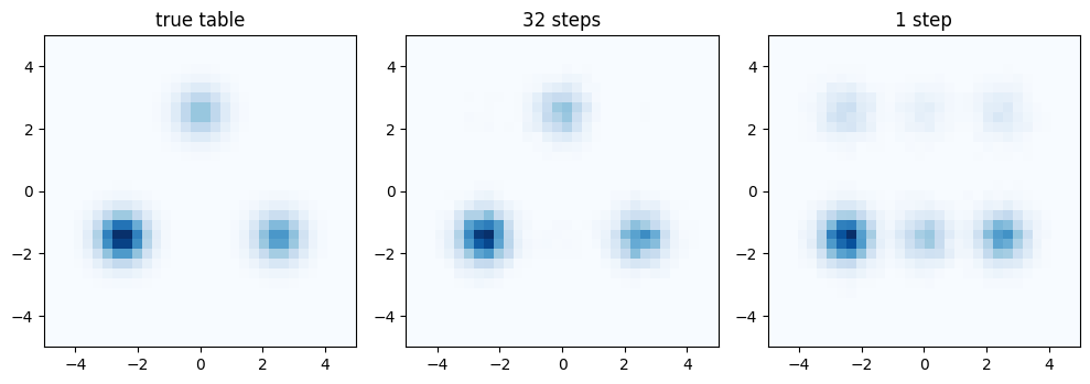
17.11.5 Images as Binary Tokens
Thresholding Fashion-MNIST at half intensity makes every pixel a token with two values, and a masked image has three. The U-Net of Section 17.6 takes the one-hot encoding as three input channels and returns two output channels, the logits of the clean pixel; the loss and the sampler are those of the running example with the positions arranged on a grid, and the schedule has \(T = 100\) steps. Eight hundred updates with a moving average of the weights, as in Section 17.8, take a few minutes. After training we estimate the bound on held-out images in bits per pixel, visiting every masking level with one random mask per image and level, and compare it with the cross-entropy of the same images under a model that treats pixels as independent, with the per-pixel frequencies of the training set.
fmnist = d2l.FashionMNIST(batch_size=128)
X = (fmnist.train.data > 127).long()  # (60000, 28, 28) tokens in {0, 1}
X_test = (fmnist.val.data > 127).long()[:200]
T, MASK = 100, 2  # the schedule for images; the mask is a third value
alpha_bar = 1 - torch.arange(T + 1) / T

class MaskedUNet(nn.Module):
    """The chapter's U-Net on one-hot tokens; outputs logits of the clean pixel."""
    def __init__(self):
        super().__init__()
        self.unet = d2l.UNet(in_channels=3, out_channels=2)

    def forward(self, z, t):
        x = nn.functional.one_hot(z, 3).float().permute(0, 3, 1, 2)
        return self.unet(x, t).permute(0, 2, 3, 1)  # (n, 28, 28, 2)

def masked_image_loss(model, x0, t):  # one-sample estimate of the bound per image, nats
    masked = torch.rand(x0.shape) < (1 - alpha_bar[t])[:, None, None]
    z = torch.where(masked, MASK, x0)
    logp = torch.log_softmax(model(z, t), -1).gather(-1, x0[..., None])[..., 0]
    weight = (alpha_bar[t - 1] - alpha_bar[t]) / (1 - alpha_bar[t])
    return (T * weight[:, None, None] * -logp * masked).sum((1, 2))

torch.manual_seed(3)
net, ema = MaskedUNet(), MaskedUNet()
ema.load_state_dict(net.state_dict())
optimizer = torch.optim.Adam(net.parameters(), lr=1e-3)
for step in range(800):
    x0 = X[torch.randint(0, len(X), (128,))]
    t = torch.randint(1, T + 1, (128,))
    loss = masked_image_loss(net, x0, t).mean() / 784
    optimizer.zero_grad(), loss.backward(), optimizer.step()
    decay = min(0.999, (1 + step) / (10 + step))
    with torch.no_grad():
        for p_ema, p in zip(ema.parameters(), net.parameters()):
            p_ema.mul_(decay).add_(p, alpha=1 - decay)
    if step % 200 == 0:
        print(f'step {step:>3}: loss {loss.item():.3f} nats per pixel')

with torch.no_grad():
    bound = sum(masked_image_loss(ema, X_test, torch.full((len(X_test),), t)).mean()
                for t in range(1, T + 1)) / T
pixel = X.float().mean(0).clamp(1e-6, 1 - 1e-6)  # frequency of white per position
independent = -(torch.special.xlogy(X_test.float(), pixel)
                + torch.special.xlogy(1 - X_test.float(), 1 - pixel)).sum((1, 2)).mean()
print(f'held-out bound: {bound / 784 / math.log(2):.3f} bits per pixel; '
      f'independent pixels: {independent / 784 / math.log(2):.3f} bits per pixel')
step 0: loss 0.789 nats per pixel
step 200: loss 0.162 nats per pixel
step 400: loss 0.141 nats per pixel
step 600: loss 0.148 nats per pixel
held-out bound: 0.180 bits per pixel; independent pixels: 0.708 bits per pixelfmnist = d2l.FashionMNIST(batch_size=128)
X = (jnp.asarray(fmnist.train[0]) > 127).astype(jnp.int32) # (60000, 28, 28)
X_test = (jnp.asarray(fmnist.val[0]) > 127).astype(jnp.int32)[:200]
T, MASK = 100, 2 # the schedule for images; the mask is a third value
alpha_bar = 1 - jnp.arange(T + 1) / T
class MaskedUNet(nnx.Module):
"""The chapter's U-Net on one-hot tokens; outputs logits of the clean pixel."""
def __init__(self, rngs):
self.unet = d2l.UNet(in_channels=3, out_channels=2, rngs=rngs)
def __call__(self, z, t):
return self.unet(jax.nn.one_hot(z, 3), t) # (n, 28, 28, 2)
def masked_image_loss(model, x0, t, key): # one-sample estimate of the bound per image, nats
masked = jax.random.uniform(key, x0.shape) < (1 - alpha_bar[t])[:, None, None]
z = jnp.where(masked, MASK, x0)
logp = jnp.take_along_axis(jax.nn.log_softmax(model(z, t), -1),
x0[..., None], -1)[..., 0]
weight = (alpha_bar[t - 1] - alpha_bar[t]) / (1 - alpha_bar[t])
return (T * weight[:, None, None] * -logp * masked).sum((1, 2))
net = MaskedUNet(nnx.Rngs(3))
graphdef, ema_state = nnx.split(net)
optimizer = nnx.Optimizer(net, optax.adam(1e-3), wrt=nnx.Param)
@nnx.jit
def image_step(net, optimizer, x0, t, key):
loss, grads = nnx.value_and_grad(
lambda m: masked_image_loss(m, x0, t, key).mean() / 784)(net)
optimizer.update(net, grads)
return loss
@jax.jit
def ema_update(ema_state, state, decay):
return jax.tree_util.tree_map(lambda e, p: decay * e + (1 - decay) * p,
ema_state, state)
for step in range(800):
key, k1, k2, k3 = jax.random.split(key, 4)
x0 = X[jax.random.randint(k1, (128,), 0, len(X))]
t = jax.random.randint(k2, (128,), 1, T + 1)
loss = image_step(net, optimizer, x0, t, k3)
ema_state = ema_update(ema_state, nnx.state(net),
min(0.999, (1 + step) / (10 + step)))
if step % 200 == 0:
print(f'step {step:>3}: loss {loss:.3f} nats per pixel')
ema = nnx.merge(graphdef, ema_state)
@nnx.jit
def bound_term(model, x0, t, key):
return masked_image_loss(model, x0, t, key).mean()
bound = 0.0
for t in range(1, T + 1):
key, subkey = jax.random.split(key)
bound += bound_term(ema, X_test, jnp.full((len(X_test),), t), subkey) / T
pixel = jnp.clip(X.astype(jnp.float32).mean(0), 1e-6, 1 - 1e-6) # frequency of white
x_test = X_test.astype(jnp.float32)
independent = -(xlogy(x_test, pixel) + xlogy(1 - x_test, 1 - pixel)).sum((1, 2)).mean()
print(f'held-out bound: {bound / 784 / math.log(2):.3f} bits per pixel; '
f'independent pixels: {independent / 784 / math.log(2):.3f} bits per pixel')step 0: loss 0.672 nats per pixel
step 200: loss 0.165 nats per pixel
step 400: loss 0.148 nats per pixel
step 600: loss 0.127 nats per pixel
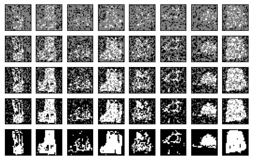
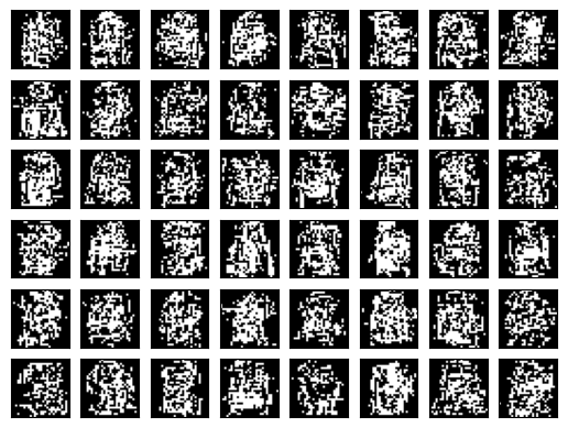
held-out bound: 0.183 bits per pixel; independent pixels: 0.708 bits per pixelThe bound is far below the independent-pixel cross-entropy: the model has captured much of the dependence between pixels that the independent model ignores. Sampling reveals the pixels over a hundred steps; the first grid shows forty-eight finished samples, the second shows eight of them at intermediate steps with masked pixels in grey, and the third uses only four steps. To quantify what the four-step sampler loses, we count speckles, pixels that differ from all four of their neighbors, in the training images and in both kinds of samples.
@torch.no_grad()
def unmask_images(model, n, steps, keep=()):
    z = torch.full((n, 28, 28), MASK)
    levels = torch.linspace(T, 0, steps + 1).round().long().tolist()
    snapshots = []
    for t, s in zip(levels[:-1], levels[1:]):
        if t in keep:
            snapshots.append(z.clone())
        draw = torch.distributions.Categorical(
            logits=model(z, torch.full((n,), t))).sample()
        reveal = (z == MASK) & (torch.rand(z.shape)
                                < (alpha_bar[s] - alpha_bar[t]) / (1 - alpha_bar[t]))
        z = torch.where(reveal, draw, z)
    return z, snapshots + [z]

def show_tokens(z, rows, cols):  # masked pixels in grey
    img = z.float().masked_fill(z == MASK, 0.5)
    d2l.show_images(img[..., None].repeat(1, 1, 1, 3), rows, cols, scale=0.8)

def speckles(z):  # fraction of interior pixels that differ from all four neighbors
    c = z[:, 1:-1, 1:-1]
    isolated = ((c != z[:, :-2, 1:-1]) & (c != z[:, 2:, 1:-1])
                & (c != z[:, 1:-1, :-2]) & (c != z[:, 1:-1, 2:]))
    return isolated.float().mean()

torch.manual_seed(4)
finished, snapshots = unmask_images(ema, 48, 100, keep=(80, 60, 40, 20))
few_steps, _ = unmask_images(ema, 48, 4)
print(f'speckles: training images {speckles(X[:1000]):.4f}, '
      f'100-step samples {speckles(finished):.4f}, '
      f'4-step samples {speckles(few_steps):.4f}')
show_tokens(finished, 6, 8)
show_tokens(torch.cat([s[:8] for s in snapshots]), 5, 8)
show_tokens(few_steps, 6, 8)
speckles: training images 0.0037, 100-step samples 0.0077, 4-step samples 0.0262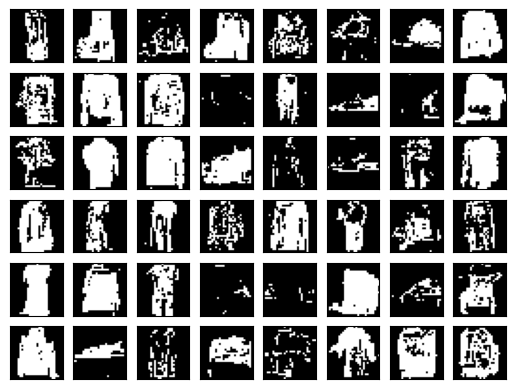
@nnx.jit
def unmask_step(model, z, t, s, key):
    k1, k2 = jax.random.split(key)
    draw = jax.random.categorical(k1, model(z, jnp.full((len(z),), t)), axis=-1)
    reveal = (z == MASK) & (jax.random.uniform(k2, z.shape)
                            < (alpha_bar[s] - alpha_bar[t]) / (1 - alpha_bar[t]))
    return jnp.where(reveal, draw, z)

def unmask_images(model, key, n, steps, keep=()):
    z = jnp.full((n, 28, 28), MASK)
    levels = [round(l) for l in jnp.linspace(T, 0, steps + 1).tolist()]
    snapshots = []
    for t, s in zip(levels[:-1], levels[1:]):
        if t in keep:
            snapshots.append(z)
        key, subkey = jax.random.split(key)
        z = unmask_step(model, z, t, s, subkey)
    return z, snapshots + [z]

def show_tokens(z, rows, cols):  # masked pixels in grey
    img = jnp.where(z == MASK, 0.5, z.astype(jnp.float32))
    d2l.show_images(jnp.repeat(img[..., None], 3, -1), rows, cols, scale=0.8)

def speckles(z):  # fraction of interior pixels that differ from all four neighbors
    c = z[:, 1:-1, 1:-1]
    isolated = ((c != z[:, :-2, 1:-1]) & (c != z[:, 2:, 1:-1])
                & (c != z[:, 1:-1, :-2]) & (c != z[:, 1:-1, 2:]))
    return isolated.mean()

key, k1, k2 = jax.random.split(key, 3)
finished, snapshots = unmask_images(ema, k1, 48, 100, keep=(80, 60, 40, 20))
few_steps, _ = unmask_images(ema, k2, 48, 4)
print(f'speckles: training images {speckles(X[:1000]):.4f}, '
      f'100-step samples {speckles(finished):.4f}, '
      f'4-step samples {speckles(few_steps):.4f}')
show_tokens(finished, 6, 8)
show_tokens(jnp.concatenate([s[:8] for s in snapshots]), 5, 8)
show_tokens(few_steps, 6, 8)
speckles: training images 0.0037, 100-step samples 0.0076, 4-step samples 0.0243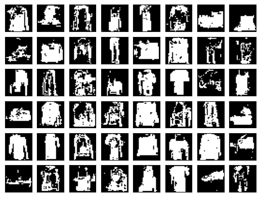
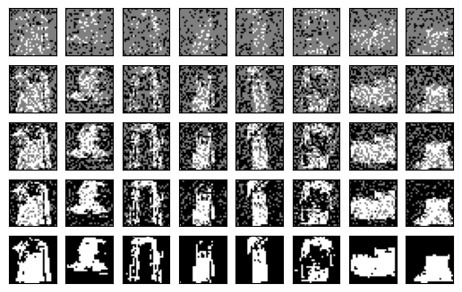
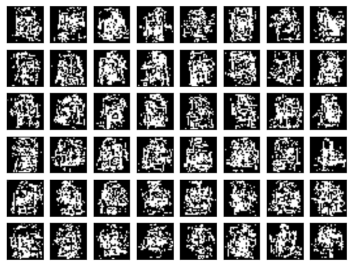
Most of the hundred-step samples are recognizable binary garments, rougher than the grey-level samples of the earlier sections, with a speckle rate about twice that of the data. The intermediate rows show the mechanism: the outline of the garment is visible once about two-fifths of the pixels are revealed, and the remaining ones fill it in consistently, because every later prediction is conditioned on everything revealed so far. The four-step samples reveal a quarter of the pixels at a time from predictions that are independent across positions, and their speckle rate is several times higher, the image counterpart of the crossed rows and columns in the one-step panel of the running example.
17.11.6 Summary
The diffusion construction does not depend on Gaussian noise. A forward Markov chain on a finite vocabulary, specified by transition matrices, has closed-form marginals and posteriors for the uniform and the absorbing kernels, and the variational bound of Section 17.7 applies as it stands. For the absorbing kernel the posterior is a two-point distribution, a masked token either stays masked or reverts to its clean value, and the bound reduces to Equation 17.11.8, a cross-entropy on masked positions with the weight \((\bar{\alpha}_{t-1} - \bar{\alpha}_t) / (1 - \bar{\alpha}_t)\), which equals \(1/t\) under the linear schedule. The network predicts clean tokens from a partially masked sequence, the task of a masked language model, and the bound makes the model a likelihood model.
Sampling reveals masked tokens step by step, never revising a revealed one. Tokens revealed in the same step are drawn independently, so fewer steps trade sequential computation for an independence error that the running example quantifies exactly: with \(S\) equally spaced steps and an exact network, a two-token model mixes in the product of the marginals with weight \(1/S\). Between one step, which draws every token independently from the prediction given the fully masked input, and one token per step, an order-agnostic autoregressive model, lies the range in which diffusion language models operate. The bound came within a few hundredths of a nat of the entropy of the quantized mixture, and the image model, the same U-Net with three input and two output channels, reached a likelihood bound far below that of independent pixels and produced binary garments by unmasking.
Several questions stay open. Which corruption suits which data is empirical: masking gave the best text likelihoods in the comparisons of Austin et al. (2021), but the uniform kernel is still trained alongside it (Lou et al. 2024), and Austin et al. (2021) also describe mixtures of the two. The bound describes a sampler that reveals tokens in uniformly random order, whereas practical samplers depart from it: Nie et al. (2025) keep the most confident predictions at each step and mask the rest again, a heuristic that the bound does not cover. Whether masked diffusion models can match autoregressive language models at equal compute, with the parallel generation that motivates them, is the subject of current work, including comparisons with autoregressive baselines trained on the same data (Nie et al. 2025).
17.11.7 Exercises
- The uniform kernel. Derive the posterior \(q(\mathbf{x}_{t-1} \mid \mathbf{x}_t, \mathbf{x}_0)\) for the uniform kernel from Equation 17.11.3 and
- Show that it depends on whether \(\mathbf{x}_t = \mathbf{x}_0\), and that for \(t \geq 2\), unlike the absorbing case, every value keeps positive probability. Why does this make the bound’s divergence terms more expensive to evaluate than Equation 17.11.8? Then show that for this kernel the two ways of averaging the posterior over the network’s prediction, the average Equation 17.11.6 and the renormalized average of the joint \(q(\mathbf{x}_{t-1}, \mathbf{x}_t \mid \hat{\mathbf{x}}_0)\) used by Austin et al. (2021), differ.
- Weights of other schedules. Compute the weight \(w_t = (\bar{\alpha}_{t-1} - \bar{\alpha}_t)/(1 - \bar{\alpha}_t)\) for the schedule \(\bar{\alpha}_t = 1 - (t/T)^2\) and compare it with \(1/t\). Which steps receive more weight, and how does the expected number of tokens revealed per step change? Then verify the substitution \(u = 1 - \bar{\alpha}(\tau)\) in the continuous-time limit and explain why the limiting bound does not depend on the schedule.
- Revealed together. Generalize the calculation of the independence error to \(L\) tokens: for the linear schedule with \(S\) equally spaced steps, compute the expected number of pairs of tokens revealed in the same step, and show that it is \(\binom{L}{2}/S\). What does this suggest about the number of steps needed for sequences of length \(L\)? Then evaluate Equation 17.11.8 for two tokens and an exact network under the linear schedule, using the three mask patterns and their probabilities, and show that it equals \(H(X^1, X^2) + I(X^1; X^2) / T\).
- [code] One token at a time. Modify
unmaskso that every step reveals exactly one masked position, chosen uniformly at random, and sample \(20{,}000\) pairs. Compare the total variation distance to the table with the thirty-two-step sampler and explain why the product term disappears. - [code] Schedules at finite \(T\). Train the pair model with the schedule \(\bar{\alpha}_t = 1 - (t/T)^2\) and compare its exact bound with that of the linear schedule. Show that an exact network attains \(H(X^1, X^2) + I(X^1; X^2) \sum_{t=1}^{T} (\bar{\alpha}_{t-1} - \bar{\alpha}_t)^2\), evaluate the sum for both schedules, and explain why the difference vanishes as \(T \to \infty\). Why does the exact prediction not depend on the time input at all?
- [code] Steps against speckles. Sample the image model with \(S \in \{100, 25, 10, 4, 1\}\) steps and plot the speckle rate against \(S\). At which point does it approach the rate of the training images, and what does that say about the number of network evaluations that masked diffusion needs for images of this size?