%matplotlib inline
from d2l import torch as d2l
import math
import time
import torch
from torch.nn import functional as F
from torch.nn.attention import SDPBackend, sdpa_kernel10.5 The Cost of Attention
Self-attention compares every query with every key, allowing information to move between any two sequence positions in one layer. For a sequence of \(n\) tokens, however, the score matrix has \(n^2\) entries. Its arithmetic and memory costs therefore grow quadratically with sequence length and can dominate long-context computation.
We first place self-attention next to the convolutional and recurrent layers of earlier chapters and make the comparison quantitative, then verify the quadratic cost of one attention layer against the actual allocator of a GPU. The remainder of the section develops three approaches. Online softmax computes exact attention without storing the full \(n \times n\) matrix and underlies FlashAttention. Sliding-window attention reduces the number of scored pairs and uses depth to increase the receptive field. Factorized kernels remove the softmax dependence between query–key pairs and yield a recurrent form related to the state space models of Section 12.2.
%matplotlib inline
from d2l import jax as d2l
import jax
from jax import numpy as jnp
import math
import time
10.5.1 CNNs, RNNs, and Self-Attention
We begin by comparing the computational properties of three sequence layers. Consider the problem of mapping a sequence of \(n\) tokens, each a \(d\)-dimensional vector, to another sequence of the same shape. Three familiar architectures can perform this mapping: a one-dimensional CNN (Chapter 6), an RNN (Section 8.4), and self-attention (Section 10.3). Figure 10.5.1 draws all three as graphs over the sequence. Two properties of these graphs matter beyond raw arithmetic. The number of sequential operations bounds how much of the work can run in parallel on modern hardware. The maximum path length counts how many layer transformations connect two positions. It is an architectural proxy, not a learnability theorem: shorter paths avoid repeatedly multiplying recurrent state Jacobians, but they do not by themselves guarantee that optimization will recover a long-range dependency.
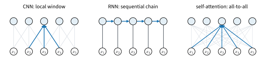
A convolutional layer with kernel size \(k\) and \(d\) channels in and out costs \(\mathcal{O}(knd^2)\) operations: each of the \(n\) positions mixes \(k\) neighbors through a \(d \times d\) map. All positions are computed at once, so there are \(\mathcal{O}(1)\) sequential steps, but the receptive field grows by only \(k-1\) positions per layer: connecting a pair of tokens \(n\) apart takes a stack of depth \(\mathcal{O}(n/k)\). An RNN requires \(\mathcal{O}(nd^2)\) for the sequence—one \(d \times d\) state update per token—but the updates are inherently ordered: \(\mathcal{O}(n)\) sequential steps, and a signal from the first token reaches the last only through \(\mathcal{O}(n)\) applications of the cell. Self-attention first projects the inputs at cost \(\mathcal{O}(nd^2)\), then computes an \(n \times d\) by \(d \times n\) product and an \(n \times n\) by \(n \times d\) product at cost \(\mathcal{O}(n^2d)\). These matrix multiplications have \(\mathcal{O}(1)\) sequential depth, and any token can attend to any other in one layer, giving path length \(\mathcal{O}(1)\). Table 10.5.1 collects the accounting.
| layer type | complexity | sequential operations | maximum path length |
|---|---|---|---|
| convolution (kernel \(k\)) | \(\mathcal{O}(knd^2)\) | \(\mathcal{O}(1)\) | \(\mathcal{O}(n/k)\) |
| recurrence | \(\mathcal{O}(nd^2)\) | \(\mathcal{O}(n)\) | \(\mathcal{O}(n)\) |
| self-attention | \(\mathcal{O}(nd^2+n^2d)\) | \(\mathcal{O}(1)\) | \(\mathcal{O}(1)\) |
Self-attention has constant sequential depth and path length, but its mixing term is quadratic in \(n\). The table includes the query, key, value, and output projections so that all three rows count the complete layer. When \(n\) and \(d\) are comparable, the linear projection and quadratic mixing terms have similar order; for \(n\gg d\), the mixing term dominates. The remainder of this section studies ways to reduce its memory use or arithmetic cost.
10.5.2 Quadratic Time and Memory
10.5.2.1 Counting FLOPs
The leading constants make this comparison more precise. One attention layer receives \(n\) queries, keys, and values of dimension \(d\) and computes Equation 10.2.6: the score matrix \(\mathbf{Q}\mathbf{K}^\top\) costs \(2n^2 d\) floating-point operations (each of the \(n^2\) entries is a length-\(d\) dot product, counting one multiply–add as two FLOPs), the softmax a few operations per entry, \(\mathcal{O}(n^2)\), and the value mixing \(\mathrm{softmax}(\cdot)\mathbf{V}\) another \(2n^2 d\). In total
\[ \underbrace{4 n^2 d}_{\textrm{scores and mixing}} + \; \mathcal{O}(n^2) \quad \textrm{FLOPs}. \tag{10.5.1}\]
Recall from Equation 10.3.3 that the projections wrapped around attention in a multi-head layer cost \(8nd^2\), which is linear in \(n\), and that the head count drops out of both terms. Setting \(4n^2d = 8nd^2\) locates the crossover: the quadratic part dominates the layer as soon as \(n > 2d\). Working the ratio for a production-sized configuration, \(d = 4096\) and \(n = 131{,}072\) give \(n/2d = 16\): an attention layer at that context does sixteen times as much score-and-mix work as projection work, and the longest-context configurations sit one to two orders of magnitude past the crossover.
10.5.2.2 Counting Memory
Arithmetic is only one part of the cost, and at inference time memory is often more important. A naive implementation materializes the score matrix and its softmax: two \(n \times n\) buffers of activations, \(8n^2\) bytes in single precision, per head and per sequence in the batch; during training the attention weights are also saved for the backward pass. The projections, by contrast, keep only \(\mathcal{O}(nd)\) activations. To feel the asymmetry: at \(n = 8192\) and a head dimension of \(d_h = 64\) — the setting of the experiments below — the inputs \(\mathbf{Q}, \mathbf{K}, \mathbf{V}\) occupy 6 MB together, while the two score buffers occupy 512 MB. At a context of \(n = 131{,}072\) tokens a single attention map in fp32 would be \(n^2 \times 4\) bytes \(\approx 69\) GB (per head, per sequence), which is why no system at that scale ever stores one.
PyTorch’s caching allocator reports exactly what a computation allocated, so we can hold the formula against reality. reset_peak_memory_stats clears the high-water mark and max_memory_allocated reads it back; we measure the d2l.DotProductAttention layer from Section 10.2 on a single head. The prediction is the two \(n \times n\) float buffers, \(8n^2\) bytes.
Measuring per-op memory at runtime is awkward in JAX, for two reasons. XLA preallocates a large fraction of GPU memory as an arena at startup (this book’s runs cap it at 40%), so device-side counters describe the arena, not the operation. The compiler may also fuse or rematerialize operations, so the buffers it materializes are determined during compilation rather than directly by the Python source. The authoritative answer therefore comes from the compiler itself: lowering a jitted function and compiling it yields a memory_analysis() report of exactly how much temporary buffer space the executable reserves. We compare it against the two \(n \times n\) float buffers, \(8n^2\) bytes.
attention = d2l.DotProductAttention(dropout=0).to(d2l.try_gpu())
attention.eval()

def peak_memory(f, *args):
    """Extra peak memory allocated by f, in bytes."""
    torch.cuda.synchronize()
    torch.cuda.reset_peak_memory_stats()
    base = torch.cuda.memory_allocated()
    f(*args)
    torch.cuda.synchronize()
    return torch.cuda.max_memory_allocated() - base

d_h = 64
for n in [2048, 4096, 8192, 16384]:
    Q = torch.randn(1, n, d_h, device=d2l.try_gpu())
    with torch.no_grad():
        measured = peak_memory(attention, Q, Q, Q)
    print(f'n = {n:5d}: measured {measured/2**20:7.1f} MiB, '
          f'predicted 8n^2 B = {8*n*n/2**20:7.1f} MiB')
n = 2048: measured 40.6 MiB, predicted 8n^2 B = 32.0 MiB
n = 4096: measured 128.0 MiB, predicted 8n^2 B = 128.0 MiB
n = 8192: measured 512.0 MiB, predicted 8n^2 B = 512.0 MiB
n = 16384: measured 2048.0 MiB, predicted 8n^2 B = 2048.0 MiBdef attention_layer(Q, K, V):
scores = Q @ K.T / math.sqrt(Q.shape[-1])
return jax.nn.softmax(scores, axis=-1) @ V
d_h = 64
for n in [2048, 4096, 8192, 16384]:
Q = jax.random.normal(jax.random.key(0), (n, d_h))
stats = jax.jit(attention_layer).lower(Q, Q, Q).compile()
temp = stats.memory_analysis().temp_size_in_bytes
print(f'n = {n:5d}: XLA temp {temp/2**20:7.1f} MiB, '
f'predicted 8n^2 B = {8*n*n/2**20:7.1f} MiB')n = 2048: XLA temp 32.0 MiB, predicted 8n^2 B = 32.0 MiB
n = 4096: XLA temp 128.0 MiB, predicted 8n^2 B = 128.0 MiB
n = 8192: XLA temp 512.0 MiB, predicted 8n^2 B = 512.0 MiB
n = 16384: XLA temp 2048.0 MiB, predicted 8n^2 B = 2048.0 MiBThe formula matches the measurement from \(n = 4096\) onward, and the XLA compiler report matches it at every size. The allocator’s smallest run (\(n = 2048\)) shows a few MiB of workspace overhead on top of the two score buffers. Doubling \(n\) quadruples the footprint. At \(n = 16{,}384\), a single fp32 head already needs 2 GB of temporary storage. The runtime has the same quadratic dependence. We time the forward pass as \(n\) doubles (after a warm-up call, and synchronizing before reading the clock—on an accelerator, kernel launches return before the work is done):
def wall_clock(f, *args, reps=10):
    f(*args)  # Warm up
    torch.cuda.synchronize()
    start = time.time()
    for _ in range(reps):
        f(*args)
    torch.cuda.synchronize()
    return (time.time() - start) / reps

for n in [2048, 4096, 8192, 16384]:
    Q = torch.randn(1, n, d_h, device=d2l.try_gpu())
    with torch.no_grad():
        t = wall_clock(attention, Q, Q, Q)
    print(f'n = {n:5d}: {t*1e3:6.2f} ms')
n = 2048: 0.15 ms
n = 4096: 0.47 ms
n = 8192: 1.84 ms
n = 16384: 7.37 msdef wall_clock(f, *args, reps=10):
f(*args).block_until_ready() # Warm up (and compile)
start = time.time()
for _ in range(reps):
f(*args).block_until_ready()
return (time.time() - start) / reps
layer = jax.jit(attention_layer)
for n in [2048, 4096, 8192, 16384]:
Q = jax.random.normal(jax.random.key(0), (n, d_h))
print(f'n = {n:5d}: {wall_clock(layer, Q, Q, Q)*1e3:6.2f} ms')n = 2048: 0.16 ms
n = 4096: 0.37 ms
n = 8192: 1.37 ms
n = 16384: 4.99 msAt small \(n\), the timings change little because the GPU is not saturated and launch overhead dominates. Beyond a few thousand tokens, each doubling of \(n\) roughly quadruples the time, consistent with the \(4n^2d\) operation count. (Accounting at the level of a whole model, including the allocation of FLOPs among parameters and data, is the subject of the scaling-laws discussion in the next chapter; here we stay inside one layer.)
10.5.3 Exact Attention Without the Matrix
10.5.3.1 Blockwise Online Softmax
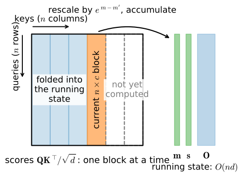
The full \(n \times n\) matrix need not be stored. The apparent obstacle to computing attention piecewise seems to be the softmax, since each weight \(\exp(a_j)/\sum_{j'}\exp(a_{j'})\) depends on all scores of its row through the normalizer and, for numerical safety, through the row maximum subtracted before exponentiation. Both quantities can be maintained online, the way one computes a running mean (Milakov and Gimelshein 2018). Process the keys in blocks and keep, per query, three running statistics: the maximum \(m\) seen so far, the sum \(s\) of exponentials rescaled to that maximum, and the output accumulator \(\mathbf{o}\). A new block of scores \(\{a_j\}\) with values \(\{\mathbf{v}_j\}\) updates them as
\[ \begin{aligned} m' &= \max\big(m, \max_j a_j\big), \\ s' &= s\, e^{m - m'} + \sum\nolimits_j e^{a_j - m'}, \\ \mathbf{o}' &= \mathbf{o}\, e^{m - m'} + \sum\nolimits_j e^{a_j - m'}\, \mathbf{v}_j, \end{aligned} \tag{10.5.2}\]
and after the last block, \(\mathbf{o}/s\) is exactly \(\mathrm{softmax}(\mathbf{a})\mathbf{V}\): whenever a new block raises the maximum, the factor \(e^{m - m'}\) rescales all quantities accumulated under the old maximum. No approximation is made. Figure 10.5.2 shows the resulting schedule: one \(n \times c\) stripe of the score matrix in memory at a time, against a running state of size \(\mathcal{O}(nd)\) (Rabe and Staats 2021).
10.5.3.2 A Chunked Implementation
From here on we work in the causal setting of a language model, masking with the dtype-safe idiom of Section 10.2. We first implement a naive reference and then a chunked version. The chunked implementation applies Equation 10.5.2 to all queries at once and processes one key block per iteration.
def causal_attention(Q, K, V):
    """Reference: causal attention with the full score matrix."""
    d = Q.shape[-1]
    i = torch.arange(Q.shape[0], device=Q.device)
    scores = Q @ K.T / math.sqrt(d)
    scores.masked_fill_(i[None, :] > i[:, None], torch.finfo(Q.dtype).min)
    return torch.softmax(scores, dim=-1) @ V

def chunked_attention(Q, K, V, chunk_size=512):
    """Exact causal attention, one n-by-chunk_size block at a time."""
    d, n = Q.shape[-1], Q.shape[0]
    m = torch.full((n, 1), torch.finfo(Q.dtype).min, device=Q.device)
    s = torch.zeros(n, 1, device=Q.device)
    O = torch.zeros(n, V.shape[-1], device=Q.device)
    pos_q = torch.arange(n, device=Q.device)[:, None]
    for start in range(0, n, chunk_size):
        Kc, Vc = K[start:start + chunk_size], V[start:start + chunk_size]
        pos_k = torch.arange(start, start + Kc.shape[0], device=Q.device)
        scores = Q @ Kc.T / math.sqrt(d)
        scores.masked_fill_(pos_k[None, :] > pos_q, torch.finfo(Q.dtype).min)
        m_new = torch.maximum(m, scores.max(dim=-1, keepdim=True).values)
        scale = torch.exp(m - m_new)                  # Rescale the past
        P = torch.exp(scores - m_new)
        s = s * scale + P.sum(dim=-1, keepdim=True)
        O = O * scale + P @ Vc
        m = m_new
    return O / s
def causal_attention(Q, K, V):
"""Reference: causal attention with the full score matrix."""
d = Q.shape[-1]
i = jnp.arange(Q.shape[0])
scores = Q @ K.T / math.sqrt(d)
scores = jnp.where(i[None, :] > i[:, None],
jnp.finfo(scores.dtype).min, scores)
return jax.nn.softmax(scores, axis=-1) @ V
def chunked_attention(Q, K, V, chunk_size=512):
"""Exact causal attention, one n-by-chunk_size block at a time."""
d, n = Q.shape[-1], Q.shape[0]
pos_q = jnp.arange(n)[:, None]
def block(carry, chunk):
m, s, O, start = carry
Kc, Vc = chunk
pos_k = start + jnp.arange(Kc.shape[0])
scores = Q @ Kc.T / math.sqrt(d)
scores = jnp.where(pos_k[None, :] > pos_q,
jnp.finfo(scores.dtype).min, scores)
m_new = jnp.maximum(m, scores.max(axis=-1, keepdims=True))
scale = jnp.exp(m - m_new) # Rescale the past
P = jnp.exp(scores - m_new)
s = s * scale + P.sum(axis=-1, keepdims=True)
O = O * scale + P @ Vc
return (m_new, s, O, start + Kc.shape[0]), None
init = (jnp.full((n, 1), jnp.finfo(Q.dtype).min), jnp.zeros((n, 1)),
jnp.zeros((n, V.shape[-1])), 0)
# The scan needs equal-sized blocks (the PyTorch loop handles a tail)
assert n % chunk_size == 0, 'n must be a multiple of chunk_size'
chunks = (K.reshape(-1, chunk_size, d),
V.reshape(-1, chunk_size, V.shape[-1]))
(m, s, O, _), _ = jax.lax.scan(block, init, chunks)
return O / sExactness is the entire point, so we check it. (In JAX we pin matrix multiplications to full fp32 for the comparison; by default they run in TF32 on this hardware, which perturbs the two computations differently at the \(10^{-4}\) level.)
torch.manual_seed(0)
n, d_h = 2048, 64
Q, K, V = (torch.randn(n, d_h, device=d2l.try_gpu()) for _ in range(3))
err = (chunked_attention(Q, K, V) - causal_attention(Q, K, V)).abs().max()
print(f'maximum deviation: {float(err):.2e}')
maximum deviation: 4.77e-07n, d_h = 2048, 64
Q, K, V = (jax.random.normal(k, (n, d_h))
for k in jax.random.split(jax.random.key(0), 3))
with jax.default_matmul_precision('highest'):
err = jnp.abs(chunked_attention(Q, K, V)
- causal_attention(Q, K, V)).max()
print(f'maximum deviation: {float(err):.2e}')maximum deviation: 4.62e-07The two computations agree up to floating-point rounding, around \(10^{-7}\) in fp32. Chunking therefore changes the evaluation order rather than the attention definition. The chunked version touches \(n \times c\) scores at a time instead of \(n \times n\), so its footprint should grow linearly in \(n\) rather than quadratically:
lengths, mems = [2048, 4096, 8192, 16384], [[], []]
for n in lengths:
    Q = torch.randn(n, d_h, device=d2l.try_gpu())
    mems[0].append(peak_memory(causal_attention, Q, Q, Q) / 2**20)
    mems[1].append(peak_memory(chunked_attention, Q, Q, Q) / 2**20)
d2l.plot(lengths, mems, 'sequence length n', 'peak memory (MiB)',
         legend=['full matrix', 'chunked'], xscale='log', yscale='log')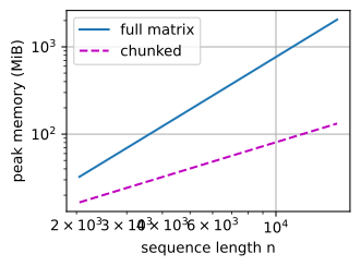
lengths, mems = [2048, 4096, 8192, 16384], [[], []]
for n in lengths:
    Q = jax.random.normal(jax.random.key(0), (n, d_h))
    for i, f in enumerate([causal_attention, chunked_attention]):
        stats = jax.jit(f).lower(Q, Q, Q).compile()
        mems[i].append(stats.memory_analysis().temp_size_in_bytes / 2**20)
d2l.plot(lengths, mems, 'sequence length n', 'XLA temp memory (MiB)',
         legend=['full matrix', 'chunked'], xscale='log', yscale='log')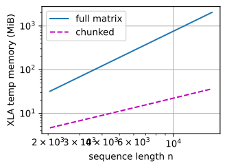
At \(n = 16{,}384\) the full-matrix implementation needs about 2 GB of scratch; the chunked one is more than an order of magnitude smaller, and the gap doubles with every further doubling of \(n\). The result and \(4n^2d\) FLOP count are unchanged; only the summation order and memory schedule differ.
10.5.3.3 Memory Traffic as the Computational Bottleneck
Chunking also reduces data movement. On a modern GPU, memory bandwidth often limits attention more than arithmetic throughput: an accelerator can execute hundreds of arithmetic operations in the time it takes to fetch one float from off-chip memory. Naive attention writes the \(n^2\) score matrix to slow memory and reads it back for the softmax and again for the value mixing. The chunked schedule keeps each stripe in fast on-chip memory, finishes all work on it, and never writes it out. FlashAttention (Dao et al. 2022) is this algorithm engineered to the hardware: tile sizes matched to on-chip SRAM, softmax statistics kept in registers. During training, the backward pass recomputes the stripes instead of storing the weights because this additional arithmetic costs less than the avoided memory traffic. The result is exact attention that is faster and asymptotically smaller, and it ships in every framework as a fused kernel: torch.nn.functional.scaled_dot_product_attention in PyTorch, jax.nn.dot_product_attention in JAX. We compare it with the naive implementation in a representative configuration (8 heads of dimension 64, half precision, \(n = 8192\)):
B, H, n = 2, 8, 8192
X = torch.randn(B, H, n, d_h, device=d2l.try_gpu(), dtype=torch.float16)

def naive_heads(X):
    i = torch.arange(X.shape[-2], device=X.device)
    scores = X @ X.transpose(-1, -2) / math.sqrt(X.shape[-1])
    scores.masked_fill_(i[None, :] > i[:, None], torch.finfo(X.dtype).min)
    return torch.softmax(scores, dim=-1) @ X

def fused_heads(X):
    with sdpa_kernel(SDPBackend.FLASH_ATTENTION):
        return F.scaled_dot_product_attention(X, X, X, is_causal=True)

for name, f in [('naive', naive_heads), ('fused', fused_heads)]:
    t, mem = wall_clock(f, X), peak_memory(f, X)
    print(f'{name}: {t*1e3:6.2f} ms, peak memory {mem/2**20:7.1f} MiB')
naive: 19.79 ms, peak memory 4112.1 MiB
fused: 1.05 ms, peak memory 16.5 MiBB, H, n = 2, 8, 8192
X = jax.random.normal(jax.random.key(0), (B, n, H, d_h), dtype=jnp.float16)
def naive_heads(X):
Xt = X.transpose(0, 2, 1, 3)
i = jnp.arange(X.shape[1])
scores = Xt @ Xt.swapaxes(-1, -2) / math.sqrt(X.shape[-1])
scores = jnp.where(i[None, :] > i[:, None],
jnp.finfo(scores.dtype).min, scores)
return (jax.nn.softmax(scores, axis=-1) @ Xt).transpose(0, 2, 1, 3)
def fused_heads(X):
return jax.nn.dot_product_attention(X, X, X, is_causal=True,
implementation='cudnn')
for name, f in [('naive', naive_heads), ('fused', fused_heads)]:
jitted = jax.jit(f)
temp = jitted.lower(X).compile().memory_analysis().temp_size_in_bytes
print(f'{name}: {wall_clock(jitted, X)*1e3:6.2f} ms, '
f'XLA temp {temp/2**20:7.1f} MiB')naive: 9.86 ms, XLA temp 4096.0 MiB
fused: 1.38 ms, XLA temp 0.0 MiBOn one GPU in half precision with the FlashAttention backend, the fused kernel is more than ten times faster than the naive implementation and uses hundreds of times less temporary memory: megabytes rather than gigabytes. Both improvements result from keeping the score blocks out of off-chip memory. Production systems therefore use fused kernels for dense attention on sequences beyond a few hundred tokens.
On one GPU in half precision with the cuDNN backend, the fused kernel is several times faster than the naive implementation. The compiler report also shows that the naive version reserves gigabytes of temporary memory for score matrices, whereas the fused kernel keeps score blocks in on-chip memory. Production systems therefore use fused kernels for dense attention on sequences beyond a few hundred tokens.
10.5.4 Windowed and Sparse Attention
10.5.4.1 Sliding-Window Attention
FlashAttention removes the \(n^2\) memory, but every query still scores every key: the arithmetic remains quadratic. To cut that too, we must decide that some query–key pairs are not worth scoring, and the simplest useful decision is locality: let each query attend only to the \(w\) most recent positions. In the masking framework of Section 10.2, the causal mask becomes a band:
n, w = 12, 4
i = torch.arange(n)
band = (i[None, :] <= i[:, None]) & (i[:, None] - i[None, :] < w)
torch.manual_seed(0)
scores = torch.randn(n, n).masked_fill(~band, torch.finfo(torch.float32).min)
d2l.show_heatmaps(torch.softmax(scores, -1)[None, None],
                  xlabel='Keys', ylabel='Queries')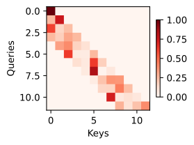
n, w = 12, 4
i = jnp.arange(n)
band = (i[None, :] <= i[:, None]) & (i[:, None] - i[None, :] < w)
scores = jax.random.normal(jax.random.key(0), (n, n))
scores = jnp.where(band, scores, jnp.finfo(scores.dtype).min)
d2l.show_heatmaps(jax.nn.softmax(scores, axis=-1)[None, None],
                  xlabel='Keys', ylabel='Queries')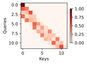
10.5.4.2 Receptive Field Growth with Depth
A window of width \(w\) excludes direct interactions beyond \(w\) tokens, but depth increases the receptive field as in CNNs (Chapter 6). A query in layer 2 attends to keys that are themselves layer-1 outputs, each of which already summarizes its own window; information therefore hops up to \(w-1\) positions per layer, and after \(L\) layers a token’s receptive field spans \(1 + L(w-1)\) positions. We can compute this rather than assert it: the band mask, read as an adjacency matrix, composes across layers by boolean matrix multiplication, and the \(L\)-th power says who can influence whom through \(L\) layers.
n, w, depths = 64, 8, [1, 2, 4]
i = torch.arange(n)
band = ((i[None, :] <= i[:, None])
        & (i[:, None] - i[None, :] < w)).float()
reach, maps = torch.eye(n), []
for L in range(1, max(depths) + 1):
    reach = ((reach @ band) > 0).float()
    if L in depths:
        maps.append(reach)
        print(f'depth {L}: last query reaches {int(reach[-1].sum())} '
              f'positions (formula: {min(n, 1 + L * (w - 1))})')
d2l.show_heatmaps(torch.stack(maps)[None], xlabel='Influencing position',
                  ylabel='Position', titles=[f'depth {L}' for L in depths],
                  figsize=(9, 3))
depth 1: last query reaches 8 positions (formula: 8)
depth 2: last query reaches 15 positions (formula: 15)
depth 4: last query reaches 29 positions (formula: 29)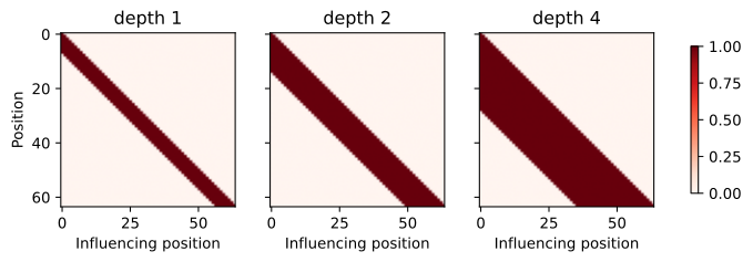
n, w, depths = 64, 8, [1, 2, 4]
i = jnp.arange(n)
band = ((i[None, :] <= i[:, None])
        & (i[:, None] - i[None, :] < w)).astype(jnp.float32)
reach, maps = jnp.eye(n), []
for L in range(1, max(depths) + 1):
    reach = ((reach @ band) > 0).astype(jnp.float32)
    if L in depths:
        maps.append(reach)
        print(f'depth {L}: last query reaches {int(reach[-1].sum())} '
              f'positions (formula: {min(n, 1 + L * (w - 1))})')
d2l.show_heatmaps(jnp.stack(maps)[None], xlabel='Influencing position',
                  ylabel='Position', titles=[f'depth {L}' for L in depths],
                  figsize=(9, 3))
depth 1: last query reaches 8 positions (formula: 8)
depth 2: last query reaches 15 positions (formula: 15)
depth 4: last query reaches 29 positions (formula: 29)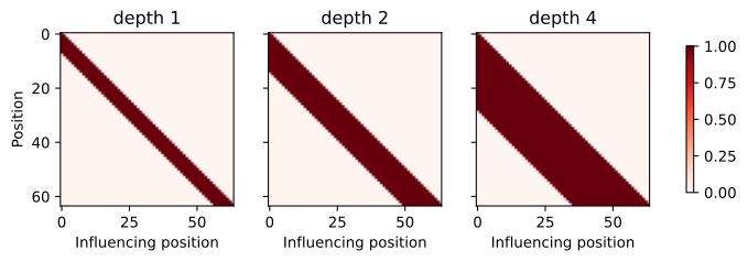
The count matches the formula exactly, and the heatmaps show the band widening layer by layer. This is precisely the bet made by deployed sliding-window models: Mistral 7B attends through a window of 4096 across 32 layers, for a theoretical reach beyond a hundred thousand tokens (Jiang et al. 2023), and Longformer combined a local window with a handful of global tokens to process whole documents (Beltagy et al. 2020), following the strided-and-local patterns of Child et al. (2019). The trade is the table of Table 10.5.1 in miniature: windowed attention gives up the \(\mathcal{O}(1)\) path length that made attention attractive, keeping \(\mathcal{O}(n/w)\) instead. With \(w\) in the thousands, this design assumes that few dependencies require more than a small number of hops.
10.5.4.3 A Linear-Cost Implementation
As with online softmax, the mask defines the semantics but not the savings: masked_softmax over a band still scores all \(n^2\) pairs and then discards most of them. The efficient implementation processes the sequence in blocks of \(w\) queries; a query in block \(b\) can only attend to keys in blocks \(b-1\) and \(b\), so each block scores a \(w \times 2w\) tile and the total work is \(2nw\) scores instead of \(n^2\), which is linear in \(n\) for fixed \(w\).
def windowed_attention(Q, K, V, w):
    """Causal sliding-window attention in O(nw) time and memory."""
    d, n = Q.shape[-1], Q.shape[0]
    assert n % w == 0, 'blocks must tile the sequence exactly'
    Qb = Q.reshape(-1, w, d)                       # (n/w, w, d) query blocks
    KV = torch.cat([torch.zeros(w, 2 * d, device=Q.device, dtype=K.dtype),
                    torch.cat([K, V], dim=-1)])   # Zero-pad one block
    idx = (torch.arange(n // w, device=Q.device)[:, None] * w
           + torch.arange(2 * w, device=Q.device)[None, :])
    KVb = KV[idx]                                  # (n/w, 2w, 2d) key blocks
    Kb, Vb = KVb[..., :d], KVb[..., d:]
    scores = Qb @ Kb.transpose(-1, -2) / math.sqrt(d)
    i = torch.arange(w, device=Q.device)[:, None]         # Query in block
    j = torch.arange(2 * w, device=Q.device)[None, :] - w  # Key offset
    block = torch.arange(n // w, device=Q.device)[:, None, None]
    valid = (j <= i) & (i - j < w) & (block * w + j >= 0)
    scores = scores.masked_fill(~valid, torch.finfo(Q.dtype).min)
    return (torch.softmax(scores, dim=-1) @ Vb).reshape(n, d)
def windowed_attention(Q, K, V, w):
"""Causal sliding-window attention in O(nw) time and memory."""
d, n = Q.shape[-1], Q.shape[0]
assert n % w == 0, 'blocks must tile the sequence exactly'
Qb = Q.reshape(-1, w, d) # (n/w, w, d) query blocks
KV = jnp.concatenate([jnp.zeros((w, 2 * d), dtype=K.dtype),
jnp.concatenate([K, V], axis=-1)]) # Zero-pad
idx = jnp.arange(n // w)[:, None] * w + jnp.arange(2 * w)[None, :]
KVb = KV[idx] # (n/w, 2w, 2d) key blocks
Kb, Vb = KVb[..., :d], KVb[..., d:]
scores = Qb @ Kb.swapaxes(-1, -2) / math.sqrt(d)
i = jnp.arange(w)[:, None] # Query in block
j = jnp.arange(2 * w)[None, :] - w # Key offset
block = jnp.arange(n // w)[:, None, None]
valid = (j <= i) & (i - j < w) & (block * w + j >= 0)
scores = jnp.where(valid, scores, jnp.finfo(scores.dtype).min)
return (jax.nn.softmax(scores, axis=-1) @ Vb).reshape(n, d)The blocked version should agree with the mask-based definition while using a lower-cost evaluation schedule:
n, w = 2048, 128
torch.manual_seed(0)
Q, K, V = (torch.randn(n, d_h, device=d2l.try_gpu()) for _ in range(3))
scores = Q @ K.T / math.sqrt(d_h)
i = torch.arange(n, device=d2l.try_gpu())
band = (i[None, :] <= i[:, None]) & (i[:, None] - i[None, :] < w)
scores.masked_fill_(~band, torch.finfo(Q.dtype).min)
reference = torch.softmax(scores, dim=-1) @ V
err = (windowed_attention(Q, K, V, w) - reference).abs().max()
print(f'maximum deviation: {float(err):.2e}')
maximum deviation: 4.17e-07n, w = 2048, 128
Q, K, V = (jax.random.normal(k, (n, d_h))
for k in jax.random.split(jax.random.key(0), 3))
with jax.default_matmul_precision('highest'):
i = jnp.arange(n)
band = (i[None, :] <= i[:, None]) & (i[:, None] - i[None, :] < w)
scores = jnp.where(band, Q @ K.T / math.sqrt(d_h),
jnp.finfo(jnp.float32).min)
reference = jax.nn.softmax(scores, axis=-1) @ V
err = jnp.abs(windowed_attention(Q, K, V, w) - reference).max()
print(f'maximum deviation: {float(err):.2e}')maximum deviation: 2.38e-07Fixed windows are the crudest possible sparsity pattern: position decides what may be attended, before the content is seen. The current frontier makes the sparsity pattern itself trainable. DeepSeek’s natively sparse attention learns which blocks each query should visit, under the same hardware-aligned block structure used here (Yuan et al. 2025).
10.5.5 Linear Attention in Recurrent Form
10.5.5.1 Kernelizing the Score
The third escape route attacks the softmax itself. Recall from Section 10.1 that attention began life as kernel regression, with weights proportional to a similarity kernel; the exponentiated dot product \(\exp(\mathbf{q}^\top\mathbf{k}/\sqrt{d})\) is one kernel among many. Suppose we choose instead a kernel that factorizes, \(k(\mathbf{q}, \mathbf{k}) = \phi(\mathbf{q})^\top \phi(\mathbf{k})\) for some elementwise feature map \(\phi\). Causal attention with this kernel is
\[ \mathbf{o}_t = \frac{\sum_{s \leq t} \phi(\mathbf{q}_t)^\top \phi(\mathbf{k}_s)\, \mathbf{v}_s} {\sum_{s \leq t} \phi(\mathbf{q}_t)^\top \phi(\mathbf{k}_s)} = \frac{\phi(\mathbf{q}_t)^\top \mathbf{S}_t} {\phi(\mathbf{q}_t)^\top \mathbf{z}_t}, \qquad \mathbf{S}_t = \sum_{s \leq t} \phi(\mathbf{k}_s) \mathbf{v}_s^\top, \quad \mathbf{z}_t = \sum_{s \leq t} \phi(\mathbf{k}_s). \tag{10.5.3}\]
Because the query enters linearly, it factors out of the sum. The remaining terms, \(\mathbf{S}_t\) and \(\mathbf{z}_t\), do not depend on the query. Reordering the sums therefore removes the explicit pairwise interaction and its quadratic cost: instead of \(t\) scores per query, one matrix-vector product against a running summary (Katharopoulos et al. 2020). Following that paper, we take \(\phi(x) = \mathrm{elu}(x) + 1\), which keeps features positive so that the normalizer cannot vanish.
The sums in Equation 10.5.3 satisfy the recurrences
\[ \mathbf{S}_t = \mathbf{S}_{t-1} + \phi(\mathbf{k}_t)\, \mathbf{v}_t^\top, \qquad \mathbf{z}_t = \mathbf{z}_{t-1} + \phi(\mathbf{k}_t), \tag{10.5.4}\]
a recurrence: a fixed-size state of \(d \times d\) numbers, updated by an outer-product write as each token arrives, then read by the query. Linear attention is a recurrent network whose hidden state is a matrix. The state acts as an associative memory, with \(\phi(\mathbf{k}_t)\) the address and \(\mathbf{v}_t\) the content, an idea that reaches back to the fast weight programmers of the early 1990s (Schlag et al. 2021). The same computation therefore has two implementations: a parallel form for training, which computes all states at once with cumulative sums, and a recurrent form for generation, which carries \((\mathbf{S}, \mathbf{z})\) forward one token at a time, in constant memory, like every RNN in Chapter 8.
def phi(X):
    return F.elu(X) + 1

def linear_attention_parallel(Q, K, V):
    """Training form: all outputs at once via cumulative sums."""
    Qp, Kp = phi(Q), phi(K)
    S = torch.cumsum(Kp[:, :, None] * V[:, None, :], dim=0)  # (n, d, d_v)
    z = torch.cumsum(Kp, dim=0)                              # (n, d)
    return (Qp[:, :, None] * S).sum(1) / (Qp * z).sum(-1, keepdim=True)

def linear_attention_recurrent(Q, K, V):
    """Generation form: a (d, d_v) state, updated token by token."""
    Qp, Kp = phi(Q), phi(K)
    S = torch.zeros(Q.shape[-1], V.shape[-1], device=Q.device)
    z = torch.zeros(Q.shape[-1], device=Q.device)
    outputs = []
    for t in range(Q.shape[0]):
        S = S + Kp[t][:, None] * V[t][None, :]   # Outer-product write
        z = z + Kp[t]
        outputs.append(Qp[t] @ S / (Qp[t] @ z))  # Query the memory
    return torch.stack(outputs)
def phi(X):
return jax.nn.elu(X) + 1
def linear_attention_parallel(Q, K, V):
"""Training form: all outputs at once via cumulative sums."""
Qp, Kp = phi(Q), phi(K)
S = jnp.cumsum(Kp[:, :, None] * V[:, None, :], axis=0) # (n, d, d_v)
z = jnp.cumsum(Kp, axis=0) # (n, d)
return (Qp[:, :, None] * S).sum(1) / (Qp * z).sum(-1, keepdims=True)
def linear_attention_recurrent(Q, K, V):
"""Generation form: a (d, d_v) state, updated token by token."""
Qp, Kp = phi(Q), phi(K)
def step(carry, qkv):
S, z = carry
q, k, v = qkv
S = S + k[:, None] * v[None, :] # Outer-product write
z = z + k
return (S, z), q @ S / (q @ z) # Query the memory
init = (jnp.zeros((Q.shape[-1], V.shape[-1])), jnp.zeros(Q.shape[-1]))
_, outputs = jax.lax.scan(step, init, (Qp, Kp, V))
return outputsEquations Equation 10.5.4 and Equation 10.5.3 sum the same terms in different orders. Their implementations therefore agree up to floating-point rounding:
torch.manual_seed(0)
n = 512
Q, K, V = (torch.randn(n, d_h, device=d2l.try_gpu()) for _ in range(3))
err = (linear_attention_parallel(Q, K, V)
       - linear_attention_recurrent(Q, K, V)).abs().max()
print(f'maximum deviation: {float(err):.2e}')
print(f'recurrent state: {d_h}x{d_h} + {d_h} floats '
      f'= {(d_h * d_h + d_h) * 4 / 1024:.0f} KiB at any sequence length')
maximum deviation: 2.38e-07
recurrent state: 64x64 + 64 floats = 16 KiB at any sequence lengthn = 512
Q, K, V = (jax.random.normal(k, (n, d_h))
for k in jax.random.split(jax.random.key(0), 3))
err = jnp.abs(linear_attention_parallel(Q, K, V)
- linear_attention_recurrent(Q, K, V)).max()
print(f'maximum deviation: {float(err):.2e}')
print(f'recurrent state: {d_h}x{d_h} + {d_h} floats '
f'= {(d_h * d_h + d_h) * 4 / 1024:.0f} KiB at any sequence length')maximum deviation: 2.38e-07
recurrent state: 64x64 + 64 floats = 16 KiB at any sequence lengthAt generation time this linear-attention layer carries 16 KiB of state, independent of context length for \(d_h=64\). A softmax head instead caches every past key and value: \(2nd_h\cdot4\) bytes in fp32, or about 4 MiB at \(n=8192\). Its cache therefore grows linearly with the generated sequence, whereas the recurrent state above remains fixed.
The state \(\mathbf{S}_t\) is a lossy summary. All past values are represented by \(d \times d\) numbers, so retrieval of one specific token can degrade as the context grows. Exact attention retains all token representations and can assign a nearly one-hot softmax weight, whereas the factorized form uses a smoother polynomial kernel. Where the quality gap matters and where it does not is an empirical question. A hybrid design can retain occasional full-attention layers within a mostly linear stack, but its quality and efficiency must be evaluated for the target workload.
10.5.5.2 Measured Time and Memory
We compare time and peak memory per forward pass for the three mechanisms—dense (exact, quadratic), windowed (sparse, linear at fixed \(w\)), and linear attention’s parallel form—as the sequence grows from 512 to 16,384 tokens. These wall-clock and memory figures come from a single GPU in fp32 and shift with hardware, dtype, and kernel. The theoretical scaling predicts the shape of each curve; the milliseconds are specific to this run.
mechanisms = {'dense': causal_attention,
              'windowed (w=128)': lambda q, k, v: windowed_attention(
                  q, k, v, 128),
              'linear': linear_attention_parallel}
lengths = [512, 1024, 2048, 4096, 8192, 16384]
times = {name: [] for name in mechanisms}
mems = {name: [] for name in mechanisms}
for n in lengths:
    Q = torch.randn(n, d_h, device=d2l.try_gpu())
    for name, f in mechanisms.items():
        times[name].append(wall_clock(f, Q, Q, Q) * 1e3)
        mems[name].append(peak_memory(f, Q, Q, Q) / 2**20)

fig, axes = d2l.plt.subplots(1, 2, figsize=(9, 3.2))
for ax, data, ylabel in zip(axes, [times, mems],
                            ['time (ms)', 'peak memory (MiB)']):
    for name in mechanisms:
        ax.loglog(lengths, data[name], marker='o', label=name)
    ax.set_xlabel('sequence length n')
    ax.set_ylabel(ylabel)
    ax.grid(linestyle='--', alpha=0.4)
axes[0].legend();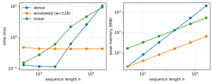
mechanisms = {'dense': jax.jit(causal_attention),
              'windowed (w=128)': jax.jit(
                  lambda q, k, v: windowed_attention(q, k, v, 128)),
              'linear': jax.jit(linear_attention_parallel)}
lengths = [512, 1024, 2048, 4096, 8192, 16384]
times = {name: [] for name in mechanisms}
mems = {name: [] for name in mechanisms}
for n in lengths:
    Q = jax.random.normal(jax.random.key(0), (n, d_h))
    for name, f in mechanisms.items():
        times[name].append(wall_clock(f, Q, Q, Q) * 1e3)
        stats = f.lower(Q, Q, Q).compile().memory_analysis()
        mems[name].append(stats.temp_size_in_bytes / 2**20)

fig, axes = d2l.plt.subplots(1, 2, figsize=(9, 3.2))
for ax, data, ylabel in zip(axes, [times, mems],
                            ['time (ms)', 'XLA temp memory (MiB)']):
    for name in mechanisms:
        ax.loglog(lengths, data[name], marker='o', label=name)
    ax.set_xlabel('sequence length n')
    ax.set_ylabel(ylabel)
    ax.grid(linestyle='--', alpha=0.4)
axes[0].legend();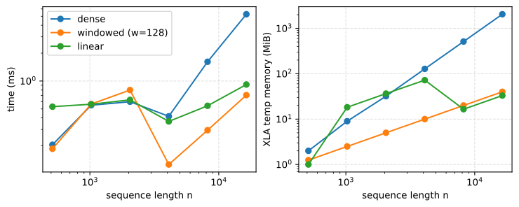
Dense attention’s curves approach slope two on the log–log axes, consistent with quadratic scaling, while the windowed mechanism’s cost is so small at these sizes that it stays pinned near the launch-overhead floor throughout. Linear attention has linear memory growth but a large \(nd_h^2\) constant because the parallel form materializes the running matrix state at every position. It uses less memory than dense attention only once \(n\) exceeds \(d_h^2\) by a sufficient margin. Its wall clock is worse than dense attention’s at moderate lengths: a cumulative sum of outer products is bandwidth-bound, while dense attention rides highly optimized matrix-multiply units, and asymptotics only pull the two level at the longest length we measure, with every further doubling tilting the balance. The decisive advantage of the linear form is the constant-memory recurrent mode at generation time, not raw training speed at moderate lengths. Production linear-attention kernels close the training gap with the same blocking tricks as FlashAttention, processing the sequence in chunks with the recurrence carried between them.
Dense attention’s curves approach slope two on the log–log axes, consistent with quadratic scaling, while the windowed mechanism’s cost stays near the launch-overhead floor at these sizes. Linear attention fares better under XLA than a bandwidth-bound cumulative sum of outer products might suggest: the compiler fuses the scan, and from \(n\) around eight thousand the linear form runs several times faster than dense attention in our measurements. Its memory column holds a small compiler lesson: at moderate lengths the reported temporaries track the parallel form’s \(nd_h^2\) state materialization, then drop at the largest sizes. XLA stops materializing the stacked outer products and streams them instead. Under a fusing compiler, what exists in memory is a scheduling decision. Both panels aside, the decisive advantage of the linear form is the constant-memory recurrent mode at generation time; production linear-attention kernels speed up training further with the same blocking tricks as FlashAttention, processing the sequence in chunks with the recurrence carried between them.
Between 2019 and 2021, several approximate attention mechanisms were proposed. Performer approximated the softmax kernel itself with random features (Choromanski et al. 2021), Linformer projected keys and values to a low-rank subspace (Wang et al. 2020), Reformer hashed similar queries and keys into shared buckets (Kitaev et al. 2020), and surveys catalogued dozens more (Tay et al. 2020). These methods are now less common in deployed systems than exact attention computed with a memory-efficient schedule (FlashAttention), restricted attention with a local sparsity pattern, and linear attention implemented as a recurrence.
10.5.5.3 Relation to State Space Models
Look once more at Equation 10.5.4. A fixed-size state, updated linearly at every step, trained in parallel, run recurrently at inference: this is precisely the linear state-space recurrence of Section 12.2, with the identity as its decay. The efficient way to train it at scale is the associative parallel scan of Section 12.2.2; give the state a learned, input-dependent decay and you have the selective models of Section 12.3. That convergence is no coincidence: Mamba-2’s state space duality makes the correspondence between selective state space models and masked attention exact (Dao and Gu 2024). Attention that retains the full history and recurrence that compresses it into a fixed-size state are two endpoints of a design space, and the mechanisms of this section—windows, chunks, matrix-state recurrences provide intermediate tradeoffs used by production systems.
10.5.6 Summary
Dense attention uses \(4n^2d\) FLOPs and, in a naive implementation, two \(n \times n\) activation buffers. Online softmax computes the same result one key block at a time while maintaining a running maximum, normalizer, and output; FlashAttention adapts this schedule to the memory hierarchy. Sliding-window attention reduces the operation count to \(\mathcal{O}(nw)\), with receptive field \(1+L(w-1)\) after \(L\) layers. A factorizing kernel yields linear attention, whose \(d \times d\) state can be computed in parallel during training or updated recurrently during generation. This state has constant inference memory but is a lossy summary of the past and connects linear attention to the state space models of Section 12.2.
10.5.7 Exercises
- Reaching across the sequence. Table 10.5.1 compares layers one at a time, but connecting two distant tokens may take many layers. Count one multiply–add as two FLOPs, so that a convolution layer with kernel \(k\) costs \(2knd^2\), an RNN layer \(4nd^2\), and a self-attention layer \(8nd^2 + 4n^2d\). Let \(n = 4096\), \(d = 512\), and \(k = 3\).
- A stack of plain convolutions must connect the first token with the last. Find the number of layers it needs and its total FLOPs, show that this total grows quadratically in \(n\), as the cost of one attention layer does, and compare the two totals numerically.
- Dilated convolutions (Section 6.3.3) with dilation \(k^{l-1}\) in layer \(l\) grow the receptive field geometrically. Find the receptive field after \(L\) layers, the depth needed to connect the two tokens, and the total FLOPs of that stack.
- Rank the four designs, namely one attention layer, the two convolution stacks, and one RNN layer, by total FLOPs and by sequential steps, counting each layer of a stack as one step and each token of the RNN as one step. Which resource does each design spend to connect the two tokens?
- The quadratic crossover. A multi-head layer costs \(8nd^2 + 4n^2 d\) FLOPs (Equation 10.3.3, Equation 10.5.1), and its two terms are equal at \(n = 2d\).
- Derive the sequence length at which the quadratic term accounts for 90% of the layer’s FLOPs, as a function of \(d\).
- Replace dense attention by a sliding window of width \(w\), and count every query as scoring \(w\) keys, as Equation 10.5.1 counts every query as scoring all \(n\) keys. Show that the attention term becomes \(4nwd\), derive the ratio of dense to windowed layer FLOPs, and find for \(d = 128\) and \(w = 4096\) the \(n\) at which the windowed layer does half the work of the dense one.
windowed_attentionscores a \(w \times 2w\) tile for every block of \(w\) queries. Compute the fraction of these scores that the maskvalidkeeps. Generalize to blocks of \(b \leq w\) queries, each scored against the \(b + w - 1\) keys that its queries can reach, and explain what limits how small \(b\) can be chosen in practice.
- [code] The running maximum. Remove the running maximum from
chunked_attention, so that the state accumulates plain sums of \(e^{a_j}\). Run the result with \(\mathbf{Q}\), \(\mathbf{K}\), \(\mathbf{V}\) and the state \(s\), \(\mathbf{O}\) in float16, on queries scaled up by a factor of \(10\).- Before running, compute the largest exponent \(x\) for which \(e^x\) is finite in float16, and estimate the fraction of scaled scores that exceed it when queries and keys of width \(64\) have independent standard normal entries.
- Run the modified function, and report at which operation the first infinite or undefined value appears.
- Explain why carrying \(m\) bounds every exponent by zero. A term \(e^{a_j - m'}\) that is smaller than the smallest positive float16 number rounds to zero. Bound the total contribution of such terms to \(s\), relative to the term of the largest score, for a row of \(n\) keys.
chunked_attentioninitializes \(m\) with the most negative finite value of the dtype and masks scores with the same value, the idiom of Section 10.2. Take \(n = 2c\) for blocks of \(c\) keys, and let the loop visit the two key blocks in reverse order, so that every score of the first visited block is masked for a query in the first block. Trace \(m\), \(s\), and \(\mathbf{O}\) for that query through both iterations, and show that the final output is still exact.
- Merging partial states. Fix one query with scores \(a_j\) and values \(\mathbf{v}_j\). For a set \(B\) of keys, call the triple \((m_B, s_B,
\mathbf{o}_B)\) that Equation 10.5.2 produces from the keys in \(B\) alone the partial state of \(B\), so that \(\mathbf{o}_B / s_B\) is the attention output restricted to \(B\).
- Derive the partial state of \(B \cup B'\) for disjoint sets \(B\) and \(B'\) from the two partial states, and show that Equation 10.5.2 is the special case in which \(B'\) is a single block.
- Show that this merge is associative and commutative. Conclude that the key blocks can be processed in any order, or in parallel and merged in a tree of depth \(\lceil \log_2 (n/c) \rceil\) for blocks of \(c\) keys, and explain why this matters when a single query attends to a long cache during generation.
- Replace the pair \((m_B, s_B)\) by the single number \(\ell_B = m_B + \log s_B\) and the triple by \((\ell_B, \bar{\mathbf{o}}_B)\) with \(\bar{\mathbf{o}}_B = \mathbf{o}_B / s_B\). Express the merged \(\ell\) and \(\bar{\mathbf{o}}\) in these terms, and show that \(\bar{\mathbf{o}}\) is a convex combination of \(\bar{\mathbf{o}}_B\) and \(\bar{\mathbf{o}}_{B'}\) whose weights depend only on \(\ell_B\) and \(\ell_{B'}\).
- Memory of chunked attention.
chunked_attentionkeeps one \(n \times c\) stripe of scores in memory at a time during the forward pass.- Assume that every operation in the loop body writes a fresh array and that an array is freed once no variable refers to it. List the arrays alive at the peak of one iteration, and express the memory beyond the inputs as \(\alpha\, nd + \beta\, nc\) floats with your values of \(\alpha\) and \(\beta\).
- Evaluate your formula for \(n = 16{,}384\), \(d = 64\), and \(c = 512\) in single precision, and compare it with the measurement in Section 10.5.3.2.
- [code] Backward memory of chunked attention. ● Training also needs the backward pass of
causal_attentionandchunked_attention.- For each of the two functions separately, differentiate the sum of its outputs with respect to \(\mathbf{Q}\), \(\mathbf{K}\), and \(\mathbf{V}\) by automatic differentiation. From the arrays that the backward pass of each operation needs, predict how much memory automatic differentiation keeps for
chunked_attentionas a function of \(n\), \(c\), and \(d\). Then measure the peak memory of the forward and backward computation of both functions for \(n \in \{2048, 4096, 8192, 16384\}\) as in Section 10.5.2.2. - Activation checkpointing (Section 5.7.2.2) of each iteration keeps only the inputs of every iteration. Count what it keeps over all \(n/c\) iterations. FlashAttention instead keeps only the output and the two statistics \(m_i\) and \(s_i\) of every query (Dao et al. 2022). Show that every attention weight can be recomputed from its score and the single number \(\ell_i = m_i + \log s_i\). Compare the floats stored by the three strategies at \(n = 16{,}384\), with FlashAttention keeping \(\ell_i\) in place of the two statistics.
- For each of the two functions separately, differentiate the sum of its outputs with respect to \(\mathbf{Q}\), \(\mathbf{K}\), and \(\mathbf{V}\) by automatic differentiation. From the arrays that the backward pass of each operation needs, predict how much memory automatic differentiation keeps for
- Traffic of a tiled schedule. ● Take the off-chip memory traffic of the naive layer to be \(4n^2\) floats, since the score matrix and the weight matrix are each written once and read once. Ignore all traffic that is linear in \(n\).
- Suppose that
chunked_attentionruns one operation at a time, each reading its inputs from off-chip memory and writing its output back. Count, as functions of \(n\), \(c\), and \(d\), the floats moved for the score stripes, the floats moved for \(\mathbf{Q}\) and the accumulator \(\mathbf{O}\), and the number of operations launched. Which of these quantities does chunking reduce relative to the naive layer? - A fused kernel instead holds a tile of \(b\) queries, their output accumulator, and one tile each of \(b\) keys and \(b\) values in an on-chip memory of \(M\) floats, so that \(4bd \leq M\); scores and per-row statistics stay in registers. It loads each query tile once, streams all key and value tiles past it, and writes each output tile once. Show that its traffic beyond the linear terms is \(2n^2 d / b\) floats and that the largest admissible tile gives \(\Theta(n^2 d^2 / M)\), the bound that Dao et al. (2022) prove for FlashAttention.
- Compute the ratio of the fused traffic to the naive traffic for \(d \in \{64, 128, 256\}\) with \(M = 2^{16}\), and state how the head width limits the benefit of tiling.
- Suppose that
- [code] Dilated windows. Longformer (Beltagy et al. 2020) combines its sliding window with dilation: a layer attends to the \(w\) positions \(t, t - r, \ldots, t - (w-1)r\), spaced \(r\) apart, as dilated convolutions do (Section 6.3.3).
- Build the dilated band mask, and recompute the receptive-field growth of Section 10.5.4.2 with \(n = 256\) and \(L = 1, \ldots, 6\) for a stack that starts with a plain window (\(w = 8\)) and alternates it with a dilated one (\(w = 8\), \(r = 4\)). Derive the closed form of the reach after \(L\) layers of this alternation.
- Repeat the computation for a stack of dilated layers only. Which offsets does it never reach, and why does alternating with a plain window fill the gaps?
- Compare the FLOP count of the alternating stack with that of a stack of plain windows that achieves the same reach.
- The cost of one more token. During generation, dense causal attention appends the new key and value to a cache of \(t\) past pairs, whereas
linear_attention_recurrentupdates a state of fixed size. Consider one head of width \(d\) in single precision.- Count the FLOPs and the bytes read from the cache to produce the output at position \(t + 1\) under dense attention.
- Count the FLOPs and the bytes of state read and written for the same step under Equation 10.5.4.
- Find the \(t\) beyond which the dense cache traffic per token exceeds the state traffic of the linear form for \(d = 64\). Compute the ratio of the two traffics at \(t = 8192\), and compare it with the ratio of the two memory sizes at that length, a 16 KiB state against a 4 MiB cache.
- A sliding-window head of width \(w\) keeps only the last \(w\) keys and values. Compare its per-token cache traffic with the state traffic of the linear form for \(d = 128\) and \(w = 4096\), and state what each of the two fixed-size memories retains about the tokens before position \(t - w\).
- [code] The feature map. The feature map \(\phi(x) =
\mathrm{elu}(x) + 1\) in
phiis one choice among many. Compare it with \(\phi(x) = \mathrm{relu}(x)\) and \(\phi(x) = \exp(x)\), both applied elementwise, on \(n = 512\) random queries and keys of widthd_h.- For each map, compute the causal linear-attention weight matrix with entries \[\frac{\phi(\mathbf{q}_t)^\top \phi(\mathbf{k}_s)}{\sum_{s' \leq t} \phi(\mathbf{q}_t)^\top \phi(\mathbf{k}_{s'})}, \qquad s \leq t,\] and measure its maximum absolute difference from the causal softmax weight matrix, which
causal_attentionforms before multiplying by \(\mathbf{V}\), and the mean entropy of its rows. - Under which condition on \(\mathbf{q}_t\) and the keys \(\mathbf{k}_1, \ldots, \mathbf{k}_t\) does the ReLU map produce an undefined row? Derive the probability of this event for row \(t\) when all entries are independent standard normal, and evaluate it for \(t = 1\) at width \(64\) and at width \(4\).
- Multiply the queries by \(\beta \in \{1, 4, 16\}\), and recompute the mean row entropy for the three maps and for the softmax weights. Explain from a property of each \(\phi\) which maps cannot sharpen their weights in this way, and what this implies for approximating a softmax row that is nearly one-hot.
- For each map, compute the causal linear-attention weight matrix with entries \[\frac{\phi(\mathbf{q}_t)^\top \phi(\mathbf{k}_s)}{\sum_{s' \leq t} \phi(\mathbf{q}_t)^\top \phi(\mathbf{k}_{s'})}, \qquad s \leq t,\] and measure its maximum absolute difference from the causal softmax weight matrix, which
- An exact feature map. ● The softmax kernel \(\kappa(\mathbf{q},
\mathbf{k}) = \exp(\mathbf{q}^\top \mathbf{k} / \sqrt{d})\) also factorizes, but only with infinitely many features.
- Expand \(\kappa\) in its Taylor series, and show that the degree-\(m\) term equals \(\phi_m(\mathbf{q})^\top \phi_m(\mathbf{k})\) for a feature map \(\phi_m\) of dimension \(d^m\) built from the \(m\)-fold tensor product of its argument.
- Truncate the series after degree \(2\). Show that the truncated kernel is positive for every pair of \(\mathbf{q}\) and \(\mathbf{k}\), so the normalizer of Equation 10.5.3 cannot vanish, and give the dimension of the feature map that concatenates \(\phi_0\), \(\phi_1\), and \(\phi_2\). For \(d = 64\) and values of width \(64\), compute the size of the state \((\mathbf{S}, \mathbf{z})\) in single precision and the length \(n\) at which the key–value cache of a softmax head reaches the same size. A truncation of this kind is the feature map of Based (Arora et al. 2024).
- Take as given that the \(n \times n\) matrix with entries \(\kappa(\mathbf{x}_i, \mathbf{x}_j)\) is positive definite for distinct \(\mathbf{x}_1, \ldots, \mathbf{x}_n\). Show that no feature map of dimension \(D < n\) reproduces \(\kappa\) exactly on these points when queries and keys coincide.
- [extended] Attention variants in a language model. ● Whether the quality gap between exact and linear attention matters depends on the task. Measure it on
TinyCharLMof Section 10.4, withpos='learned'for every variant so that position enters the same way.- Subclass
TinyCharLMand override_attendtwice: once with a causal band mask of width \(w\) in place of the causal mask, and once with the causal linear-attention weights of Equation 10.5.3 for \(\phi(x) = \mathrm{elu}(x) + 1\), computed explicitly as a \(T \times T\) matrix so that the method still returns its weights. - Train dense attention, windows of width \(w \in \{4, 16, 64\}\), and linear attention with the protocol of Section 10.4.4.3, and report validation perplexity at context \(128\). Relate the window results to the reach \(1 + 2(w-1)\) of the two-block model.
- Build validation sequences of \(128\) characters, each a random \(64\)-character excerpt of the validation text followed by the same excerpt again, and compare the mean loss on the second half with that on the first half for every variant. Which variants exploit the repetition, and how does the answer relate to the reach of the windowed models and to the fixed-size state of linear attention?
- Subclass
- [code] A decaying state. ● Give the state of Equation 10.5.4 a scalar decay \(\gamma \in (0, 1)\), \[\mathbf{S}_t = \gamma\, \mathbf{S}_{t-1} + \phi(\mathbf{k}_t)\,\mathbf{v}_t^\top, \qquad \mathbf{z}_t = \gamma\, \mathbf{z}_{t-1} + \phi(\mathbf{k}_t). \tag{10.5.5}\]
- Show that the parallel form now weights the contribution of position \(s\) to the output at \(t\) by \(\gamma^{t-s}\), and implement it by rescaling the cumulative sums of
linear_attention_parallelwith powers of \(\gamma\). - Add the decay to
linear_attention_recurrent, and verify that the two forms agree for \(n = 512\) and \(\gamma = 0.99\). - The rescaling multiplies position \(s\) by \(\gamma^{-s}\) before the cumulative sum. For which \(n\) does this overflow single precision at \(\gamma = 0.9\) and at \(\gamma = 0.5\)?
- Split the sequence into chunks of \(c\) positions, rescale each position relative to the start of its chunk, and carry the state from one chunk to the next with the decayed recurrence. Show that no factor larger than \(\gamma^{-c}\) appears, implement this chunked form for \(\gamma = 0.5\), \(n = 512\), and \(c = 64\), and compare it with the recurrent form.
- Compute the lag at which the weight \(\gamma^{t-s}\) falls below \(0.01\) for \(\gamma = 0.99\). A task requires recalling one token from \(2000\) positions back, while the tokens in between are filler. Explain why no fixed \(\gamma\) serves both that token and the filler, and what a decay computed from each token’s own input could do instead.
- Show that the parallel form now weights the contribution of position \(s\) to the output at \(t\) by \(\gamma^{t-s}\), and implement it by rescaling the cumulative sums of