import numpy as np
import torch25.3 Matrix Calculus
The previous section wrote the gradient as a column of partial derivatives and the chain rule as a sum over paths through a graph of scalars. A network is not written in scalars. Each layer maps a vector to a vector, and its weights form a matrix. What is the derivative of the loss with respect to a vector or a matrix, and how do we compute it for a whole layer at once?
A network small enough to work by hand shows what is needed. It has two inputs, two ReLU hidden units and one output,
\[ g(\mathbf x)=\mathbf w_2^\top\boldsymbol\varphi(\mathbf W_1\mathbf x+\mathbf b),\qquad \mathbf W_1=\begin{pmatrix}1&2\\3&-1\end{pmatrix},\quad \mathbf b=\begin{pmatrix}0\\-4\end{pmatrix},\quad \mathbf w_2=\begin{pmatrix}2\\-1\end{pmatrix}, \]
where \(\boldsymbol\varphi\) applies \(\max(0,\cdot)\) to each entry. At \(\mathbf x=(1,1)\) the pre-activations are \(\mathbf W_1\mathbf x+\mathbf b=(3,-2)\), so the second unit is off, the hidden vector is \((3,0)\), and the output is \(g=6\). A training step asks three questions about this number. If the input moves by \(\boldsymbol\delta\), the output changes by \(2\delta_1+4\delta_2\), a row of two numbers, the transpose of the previous section’s column gradient. If the weight matrix moves by \(\Delta\mathbf W_1\), the output changes by \(2\,\Delta W_{11}+2\,\Delta W_{12}\) and not at all through the second row, so the derivative with respect to a matrix is again a matrix, \(\left(\begin{smallmatrix}2&2\\0&0\end{smallmatrix}\right)\). And the hidden layer \(\mathbf x\mapsto\boldsymbol\varphi(\mathbf W_1\mathbf x+\mathbf b)\) maps a vector to a vector. Neither a slope nor a gradient describes its derivative, yet the output reaches \(\mathbf W_1\) only through that layer.
Such derivatives are easy to get wrong by hand. A hand-derived gradient with a transposed square factor raises no error, and training goes wrong. Reference tables of matrix derivatives run to hundreds of entries, and they do not protect against that mistake.
This section answers the three questions with one object and one rule. The derivative of a vector-valued map is a matrix, the Jacobian, defined as the map’s best linear approximation. Composing maps multiplies Jacobians, so the derivative of a network is a product of matrices, one per layer. The derivatives a layer needs (linear and quadratic forms, least squares, matrix products, softmax) all follow from one rule: write down the first-order change of the function and read the gradient off as its coefficient. The same rule produces the backward pass of each layer. We check every result against a framework’s automatic differentiation and end with \(\mathbf p-\mathbf y\), the gradient every classifier computes.
We use the following imports throughout this section.
import numpy as np
import tensorflow as tf
import numpy as np
import jax
from jax import numpy as jnpfrom mxnet import autograd, npx
from mxnet import np as mnp
import numpy as np
npx.set_np()25.3.1 The Jacobian
A scalar function of many variables has a gradient. A layer of a network is a function \(\mathbf f:\mathbb R^n\to\mathbb R^m\) with many outputs, and this part finds the object that plays the role of its derivative.
25.3.1.1 The Best Linear Approximation
The loss of a network is one number, but it depends on the first layer through every later layer, and each of those maps a vector to a vector. We start with the smallest such map that is not linear, the one this section and the next use throughout:
\[ \mathbf f(x,y)=\begin{pmatrix}x+\sin y\\ y+x^2/2\end{pmatrix},\qquad \mathbf x_0=(0.5,\ 0.5). \]
At \(\mathbf x_0\) its value is \(\mathbf f(\mathbf x_0)=(0.9794,\ 0.6250)\). Each of the two outputs has two partial derivatives: \(\partial f_1/\partial x=1\), \(\partial f_1/\partial y=\cos y=0.8776\), \(\partial f_2/\partial x=x=0.5\) and \(\partial f_2/\partial y=1\). We arrange the four numbers in a matrix with one row per output and one column per input,
\[ \mathbf J(\mathbf x_0)=\begin{pmatrix}1&\cos 0.5\\0.5&1\end{pmatrix} =\begin{pmatrix}1&0.8776\\0.5&1\end{pmatrix}. \]
Column \(j\) says how both outputs move when input \(j\) moves. The two columns point in different directions and \(\det\mathbf J=1-0.5\cdot0.8776=0.5612\), so the matrix is invertible: near \(\mathbf x_0\) the map does not fold the plane onto a line. This matrix is the derivative of \(\mathbf f\) at \(\mathbf x_0\), in the sense that \(\mathbf f(\mathbf x_0+\boldsymbol\delta)\approx\mathbf f(\mathbf x_0)+\mathbf J\boldsymbol\delta\) for small \(\boldsymbol\delta\), and no other matrix does as well.
In one variable, the derivative is the slope of the best straight-line fit, \(f(x+\delta)\approx f(x)+f'(x)\,\delta\). The vector-valued generalization uses the same local approximation. We say \(\mathbf f\) is differentiable at \(\mathbf x\) if there is a matrix \(\mathbf J\in\mathbb R^{m\times n}\) such that
\[ \mathbf f(\mathbf x+\boldsymbol\delta) = \mathbf f(\mathbf x) + \mathbf J\,\boldsymbol\delta + o(\|\boldsymbol\delta\|), \tag{25.3.1}\]
that is, the error of the linear model \(\mathbf f(\mathbf x)+\mathbf J\boldsymbol\delta\) divided by \(\|\boldsymbol\delta\|\) tends to zero as \(\boldsymbol\delta\to\mathbf 0\). That matrix, if it exists, is unique, is called the Jacobian \(\mathbf J_{\mathbf f}(\mathbf x)\), and its entries are the partial derivatives:
\[ [\mathbf J_{\mathbf f}]_{ij} = \frac{\partial f_i}{\partial x_j}. \tag{25.3.2}\]
To see why, feed Equation 25.3.1 the perturbation \(\boldsymbol\delta=t\,\mathbf e_j\) (a small step along axis \(j\)) and read off component \(i\): dividing by \(t\) and letting \(t\to0\) leaves \(\partial f_i/\partial x_j\) in the \((i,j)\) slot, whatever matrix we started with. So row \(i\) of \(\mathbf J\) collects the partials of the \(i\)-th output, and column \(j\) records how all outputs respond to nudging input \(j\). The partial derivatives supply the entries of \(\mathbf J\), but the linear approximation is what defines it.
Partials alone do not guarantee a Jacobian. The function \(f(x,y)=2xy/(x^2+y^2)\) with \(f(0,0)=0\), met in the previous section, vanishes on both axes, so both partials at the origin are \(0\). Yet \(f=1\) everywhere on the diagonal \(x=y\), arbitrarily close to the origin. The only candidate matrix is the zero row, and along the diagonal it misses \(f\) by \(1\), an error that does not shrink with \(\boldsymbol\delta\). So \(f\) has no Jacobian at the origin. A sufficient condition is continuity of the partials: if every partial \(\partial f_i/\partial x_j\) exists near \(\mathbf x\) and is continuous at \(\mathbf x\), then \(\mathbf f\) is differentiable at \(\mathbf x\) (Rudin 1976).
Figure 25.3.1 shows the definition at work: near \(\mathbf x_0\), the map acts like its Jacobian. A circle of radius \(r\) around \(\mathbf x_0\) maps nearly onto the ellipse \(\mathbf f(\mathbf x_0)+\mathbf J\boldsymbol\delta\), \(\|\boldsymbol\delta\|=r\), whose semi-axes are \(r\) times the singular values of \(\mathbf J\) (a matrix maps the unit circle to an ellipse with these semi-axes, Section 24.4). Here the singular values are \(1.706\) and \(0.329\), so the circle of radius \(0.35\) becomes an ellipse with semi-axes \(0.60\) and \(0.12\). The largest gap between the true image and the ellipse is \(0.061\) at \(r=0.35\) and \(0.015\) at \(r=0.175\): halving the radius cuts the gap fourfold.

Does the error of the linear model fall faster than \(\|\boldsymbol\delta\|\) itself? We shrink one perturbation tenfold at a time and print the error divided by \(\|\boldsymbol\delta\|\).
def f(v):                                   # the running map, R^2 -> R^2
    x, y = v
    return np.array([x + np.sin(y), y + x**2 / 2])

def J(v):                                   # its Jacobian, entry by entry
    x, y = v
    return np.array([[1.0, np.cos(y)], [x, 1.0]])

x0 = np.array([0.5, 0.5])
for s in [1, 0.1, 0.01, 0.001]:
    delta = s * np.array([0.2, 0.1])
    err = np.linalg.norm(f(x0 + delta) - f(x0) - J(x0) @ delta)
    print(f'|delta| = {np.linalg.norm(delta):.1e}   '
          f'error / |delta| = {err / np.linalg.norm(delta):.1e}')
|delta| = 2.2e-01 error / |delta| = 9.0e-02
|delta| = 2.2e-02 error / |delta| = 9.0e-03
|delta| = 2.2e-03 error / |delta| = 9.0e-04
|delta| = 2.2e-04 error / |delta| = 9.0e-05The ratio goes from \(0.09\) to \(0.009\), \(0.0009\) and \(0.00009\). It tends to zero, which is the \(o(\|\boldsymbol\delta\|)\) of the definition. It also falls tenfold for every tenfold step, so the error itself falls a hundredfold: the error is \(O(\|\boldsymbol\delta\|^2)\). The definition promises only the first property; the second holds because \(\mathbf f\) has continuous second derivatives.
25.3.1.2 Gradients, Hessians, and the Shape of a Derivative
The gradient and the Hessian of the previous section are both built from Jacobians. The gradient is the transpose of the Jacobian of a scalar function, and the Hessian is the Jacobian of the gradient. Seeing them this way settles a question of shape that every hand derivation runs into: whether a derivative is a row or a column, and how a derivative with respect to a matrix is arranged.
When \(m=1\), a scalar field \(f:\mathbb R^n\to\mathbb R\), the Jacobian is a single row, \(\partial f/\partial\mathbf x=[\partial f/\partial x_1,\ldots,\partial f/\partial x_n]\), and Equation 25.3.1 is the first-order expansion \(f(\mathbf x+\boldsymbol\delta)\approx f(\mathbf x)+(\partial f/\partial\mathbf x)\,\boldsymbol\delta\) of the previous section. That section wrote the gradient as a column. The two are transposes of each other,
\[ \nabla_{\mathbf x} f = \Bigl(\frac{\partial f}{\partial\mathbf x}\Bigr)^{\!\top}, \tag{25.3.3}\]
and this book uses both, each for one job. Jacobians of vector-valued maps are \(m\times n\), one row per output, so that the chain rule below composes without transposes. Gradients of scalars are columns, \(\nabla_{\mathbf x}f\), the vector an optimizer subtracts from \(\mathbf x\). For the network of the opening, \(\partial g/\partial\mathbf x=(2,\ 4)\) is a \(1\times2\) Jacobian and \(\nabla_{\mathbf x}g=(2,4)^\top\) is the column.
A scalar function of a matrix \(\mathbf W\in\mathbb R^{p\times q}\) needs one more convention. Its gradient \(\nabla_{\mathbf W}f\) is the \(p\times q\) matrix with entries \(\partial f/\partial W_{ij}\), so it has the shape of \(\mathbf W\). Then the first-order expansion reads
\[ f(\mathbf W+\mathbf E)=f(\mathbf W)+\langle\nabla_{\mathbf W}f,\ \mathbf E\rangle+o(\|\mathbf E\|), \qquad \langle\mathbf A,\mathbf B\rangle=\operatorname{tr}(\mathbf A^\top\mathbf B)=\sum_{ij}A_{ij}B_{ij}, \tag{25.3.4}\]
where \(\langle\cdot,\cdot\rangle\) multiplies two matrices of the same shape entry by entry and adds the products, the dot product of the matrices read as long vectors. The change of \(f\) is the sum over all entries of “sensitivity times nudge”. In the opening, \(\nabla_{\mathbf W_1}g\) is the \(2\times2\) matrix \(\left(\begin{smallmatrix}2&2\\0&0\end{smallmatrix}\right)\), and \(\langle\nabla_{\mathbf W_1}g,\Delta\mathbf W_1\rangle=2\,\Delta W_{11}+2\,\Delta W_{12}\) is the change we found there. One rule checks every formula in this section: a gradient has the shape of its variable. If a derived gradient does not, a transpose is missing.
Differentiating once more brings in the Hessian. The gradient field \(\nabla f:\mathbb R^n\to\mathbb R^n\) is itself a vector-valued map, and its Jacobian is the matrix of second partials, the Hessian \(\mathbf H_f\), with \([\mathbf H_f]_{ij}=\partial^2 f/\partial x_i\partial x_j\). The entry \([\mathbf J_{\nabla f}]_{ij}=\partial^2 f/\partial x_j\partial x_i\) takes the derivatives in the other order; the two agree, and \(\mathbf H_f\) is symmetric, when the mixed partials are continuous (the Clairaut–Schwarz theorem of the previous section).
25.3.2 The Chain Rule for Jacobians
A network is a composition of layers. The previous section’s chain rule summed over every path from an input to an output; for layers that are vector maps, that sum is a matrix product.
25.3.2.1 Composition as a Matrix Product
Proposition (chain rule). If \(\mathbf f:\mathbb R^n\to\mathbb R^p\) is differentiable at \(\mathbf x\) and \(\mathbf g:\mathbb R^p\to\mathbb R^m\) is differentiable at \(\mathbf f(\mathbf x)\), then \(\mathbf g\circ\mathbf f\) is differentiable at \(\mathbf x\) and
\[ \mathbf J_{\mathbf g\circ\mathbf f}(\mathbf x) = \mathbf J_{\mathbf g}\!\bigl(\mathbf f(\mathbf x)\bigr)\,\mathbf J_{\mathbf f}(\mathbf x). \tag{25.3.5}\]
Proof. Write \(\mathbf y=\mathbf f(\mathbf x)\) and let \(\mathbf A=\mathbf J_{\mathbf f}(\mathbf x)\), \(\mathbf B=\mathbf J_{\mathbf g}(\mathbf y)\). We substitute the linear model for \(\mathbf f\) into the linear model for \(\mathbf g\). By Equation 25.3.1, \(\mathbf f(\mathbf x+\boldsymbol\delta)=\mathbf y+\mathbf A\boldsymbol\delta +o(\|\boldsymbol\delta\|)\). Calling that displacement \(\boldsymbol\eta=\mathbf A\boldsymbol\delta+o(\|\boldsymbol\delta\|)\) and feeding it to \(\mathbf g\),
\[ \mathbf g\bigl(\mathbf f(\mathbf x+\boldsymbol\delta)\bigr) = \mathbf g(\mathbf y) + \mathbf B\,\boldsymbol\eta + o(\|\boldsymbol\eta\|) = \mathbf g(\mathbf y) + \mathbf B\mathbf A\,\boldsymbol\delta + o(\|\boldsymbol\delta\|). \]
The second equality needs two facts. \(\mathbf B\) applied to the \(o(\|\boldsymbol\delta\|)\) remainder is again \(o(\|\boldsymbol\delta\|)\). And \(\|\boldsymbol\eta\|\le\|\mathbf A\|\,\|\boldsymbol\delta\|+o(\|\boldsymbol\delta\|)\) is bounded by a constant multiple of \(\|\boldsymbol\delta\|\), so \(\mathbf g\)’s own remainder \(o(\|\boldsymbol\eta\|)\) is \(o(\|\boldsymbol\delta\|)\) as well; this is the one step that is not routine. The coefficient of \(\boldsymbol\delta\) is therefore a matrix with the property Equation 25.3.1, and by uniqueness it is the Jacobian of the composite: \(\mathbf J_{\mathbf g\circ\mathbf f}=\mathbf B\mathbf A\). \(\blacksquare\)
One entry of the product recovers the chain rule of the previous section: \([\mathbf B\mathbf A]_{ik}=\sum_j (\partial g_i/\partial y_j)(\partial f_j/\partial x_k)\) sums, over the intermediate variables \(y_j\), the product of the derivatives along each path from \(x_k\) to \(g_i\).
25.3.2.2 The Jacobian of a Network
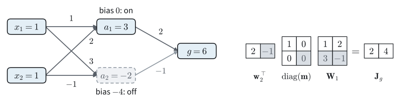
The network of the opening is a composition of three maps: the affine map \(\mathbf a=\mathbf W_1\mathbf x+\mathbf b\), the ReLU \(\mathbf h=\boldsymbol\varphi(\mathbf a)\), and the output \(g=\mathbf w_2^\top\mathbf h\). The first map is its own linear approximation, so its Jacobian is \(\mathbf W_1\); the bias shifts the value and not the slope. The ReLU acts on each entry separately, with slope \(1\) where \(a_i>0\) and \(0\) where \(a_i<0\), so its Jacobian is the diagonal matrix \(\operatorname{diag}(\mathbf m)\) of the mask \(\mathbf m\), the vector of these slopes. The output map has Jacobian \(\mathbf w_2^\top\). At \(\mathbf x=(1,1)\), where \(\mathbf a=(3,-2)\) and \(\mathbf m=(1,0)\), the chain rule multiplies the three:
\[ \mathbf J_g(\mathbf x)=\mathbf w_2^\top\operatorname{diag}(\mathbf m)\,\mathbf W_1 =\begin{pmatrix}2&-1\end{pmatrix}\begin{pmatrix}1&0\\0&0\end{pmatrix}\begin{pmatrix}1&2\\3&-1\end{pmatrix} =\begin{pmatrix}2&0\end{pmatrix}\begin{pmatrix}1&2\\3&-1\end{pmatrix} =\begin{pmatrix}2&4\end{pmatrix}. \]
The mask zeroes the second entry of \(\mathbf w_2^\top\), so the second row of \(\mathbf W_1\) never reaches the output: the weights of an inactive unit play no part in the derivative (Figure 25.3.2). The row \((2,4)\) is the change \(2\delta_1+4\delta_2\) of the opening. At another input the mask changes and so does the Jacobian. At \(\mathbf x=(2,-3)\) the pre-activations are \((-4,5)\), the mask is \((0,1)\), and \(\mathbf J_g=(0,\ -1)\,\mathbf W_1=(-3,\ 1)\). Because ReLU is piecewise linear, a finite difference along each axis reproduces these entries without error for steps small enough to keep the mask fixed; the first exercise makes this precise.
The same two kinds of factor make up every multilayer perceptron. A dense layer \(\mathbf x\mapsto\mathbf W\mathbf x\) has \(\mathbf J=\mathbf W\). An elementwise activation \(\boldsymbol\varphi(\mathbf x)=(\varphi(x_1),\ldots,\varphi(x_n))\) couples no pair of coordinates, so all off-diagonal partials vanish and \(\mathbf J_{\boldsymbol\varphi}(\mathbf x)=\operatorname{diag}\bigl(\varphi'(x_1),\ldots,\varphi'(x_n)\bigr)\). This requires \(\varphi\) to be differentiable at every \(x_i\). ReLU has no derivative at \(0\), and frameworks use a fixed value there by convention, as in the single-variable section. A network of depth \(K\) is a composition \(\mathbf f=\mathbf f_K\circ\cdots\circ\mathbf f_1\), and iterating Equation 25.3.5 turns its derivative into one product,
\[ \mathbf J = \mathbf J_K\,\mathbf J_{K-1}\cdots\mathbf J_1, \tag{25.3.6}\]
with each factor evaluated at the input of its layer. For the alternation of dense layers and activations this is \(\mathbf J=\operatorname{diag}(\boldsymbol\varphi_K')\,\mathbf W_K\cdots \operatorname{diag}(\boldsymbol\varphi_1')\,\mathbf W_1\): weight matrices interleaved with diagonal factors. Multiplying a vector by a diagonal factor scales each entry, which costs \(O(n)\) operations instead of \(O(n^2)\).
Does a framework’s automatic differentiation agree with the product \(\mathbf w_2^\top\operatorname{diag}(\mathbf m)\mathbf W_1\)? We define the network as a function of the input and of its parameters, then compare the two.
W1, b = torch.tensor([[1.0, 2.0], [3.0, -1.0]]), torch.tensor([0.0, -4.0])
w2, x = torch.tensor([2.0, -1.0]), torch.tensor([1.0, 1.0])

def g(x, W1, b, w2):                         # the 2-2-1 ReLU network
    return w2 @ torch.relu(W1 @ x + b)

m = (W1 @ x + b > 0).float()                 # the ReLU mask
print('by hand    :', (w2 @ torch.diag(m) @ W1).numpy())
print('by autograd:', torch.func.grad(g)(x, W1, b, w2).numpy())
by hand : [2. 4.]
by autograd: [2. 4.]W1, b = tf.constant([[1.0, 2.0], [3.0, -1.0]]), tf.constant([0.0, -4.0])
w2, x = tf.constant([2.0, -1.0]), tf.constant([1.0, 1.0])
def g(x, W1, b, w2): # the 2-2-1 ReLU network
return tf.tensordot(w2, tf.nn.relu(tf.linalg.matvec(W1, x) + b), 1)
m = tf.cast(tf.linalg.matvec(W1, x) + b > 0, tf.float32) # the ReLU mask
with tf.GradientTape() as tape:
tape.watch(x)
out = g(x, W1, b, w2)
print('by hand :', (w2[None, :] @ tf.linalg.diag(m) @ W1)[0].numpy())
print('by autograd:', tape.gradient(out, x).numpy())by hand : [2. 4.]
by autograd: [2. 4.]W1, b = jnp.array([[1.0, 2.0], [3.0, -1.0]]), jnp.array([0.0, -4.0])
w2, x = jnp.array([2.0, -1.0]), jnp.array([1.0, 1.0])
def g(x, W1, b, w2): # the 2-2-1 ReLU network
return w2 @ jax.nn.relu(W1 @ x + b)
m = (W1 @ x + b > 0).astype(jnp.float32) # the ReLU mask
print('by hand :', np.asarray(w2 @ jnp.diag(m) @ W1))
print('by autograd:', np.asarray(jax.grad(g)(x, W1, b, w2)))by hand : [2. 4.]
by autograd: [2. 4.]W1, b = mnp.array([[1.0, 2.0], [3.0, -1.0]]), mnp.array([0.0, -4.0])
w2, x = mnp.array([2.0, -1.0]), mnp.array([1.0, 1.0])
def g(x, W1, b, w2): # the 2-2-1 ReLU network
return mnp.dot(w2, npx.relu(mnp.dot(W1, x) + b))
m = (mnp.dot(W1, x) + b > 0).astype('float32') # the ReLU mask
x.attach_grad()
with autograd.record():
out = g(x, W1, b, w2)
out.backward()
print('by hand :', mnp.dot(mnp.dot(w2, mnp.diag(m)), W1).asnumpy())
print('by autograd:', x.grad.asnumpy())by hand : [2. 4.]
by autograd: [2. 4.]Both lines print \((2,4)\). The product Equation 25.3.6 has a limit that matters for training: it is the derivative with respect to the input. The weight matrices \(\mathbf W_k\) appear in it as factors, never as variables, so it does not say how the output changes when a weight changes. Those gradients need one more rule per layer, which Section 25.3.3.2 derives and applies to this same network.
25.3.2.3 The Order of Multiplication
Matrix multiplication is associative, so the product Equation 25.3.6 may be bracketed in any order and every order gives the same matrix. The orders differ in cost by a factor that grows with the width of the network. Training needs the gradient of a scalar loss \(\ell\), so the chain starts on the left with a row vector, the \(1\times h\) Jacobian \(\mathbf u^\top=\partial\ell/\partial\mathbf h_K\) of the loss with respect to the last layer’s output \(\mathbf h_K\). Multiplying from the left keeps every intermediate result a row vector: \(\mathbf u^\top\mathbf J_K\) is a row, that row times \(\mathbf J_{K-1}\) is a row, and so on, so every step multiplies a matrix by a vector. Multiplying from the right instead multiplies matrix by matrix until the row arrives at the end. The cheap order is the one in which every step is a matrix–vector product. If a column vector \(\mathbf v\) (one input direction) sits on the right of the chain instead, multiplying from the right is the cheap order.
A count makes the difference concrete. Take \(\mathbf u^\top\mathbf J_3\mathbf J_2\mathbf J_1\) with shapes \(1\times h\), \(h\times h\), \(h\times h\) and \(h\times n\), and \(h=n=1000\), where a \(p\times q\) matrix times a \(q\times r\) matrix costs \(pqr\) multiplications. From the left there are three matrix–vector products, \(h^2+h^2+hn=3\times10^6\) multiplications. From the right, \(\mathbf J_2\mathbf J_1\) and then \(\mathbf J_3(\mathbf J_2\mathbf J_1)\) cost \(h^2n=10^9\) each, and the final product with \(\mathbf u^\top\) costs \(hn=10^6\), in all \(2.001\times10^9\). Three million against two billion is a factor of about \(670\), or \(2h/3\) (Figure 25.3.3).
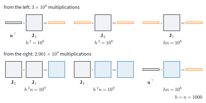
The two orders correspond to two directions through the network. Multiplying from the left carries the sensitivity of the output backward through the layers, from the last to the first, and yields the gradient of a scalar loss at the cost of one matrix–vector product per layer. Multiplying from the right, with a seed column \(\mathbf v\), carries one input direction forward through the layers and yields \(\mathbf J\mathbf v\). Programs that evaluate these two orders automatically are called reverse-mode and forward-mode automatic differentiation.
The count above uses factors of equal width. When the factors have different shapes, neither end order need be cheapest. The best bracketing of a chain is found by a dynamic program (see the exercises), while for a general computation graph finding the cheapest order is NP-complete (Naumann 2008).
The values of the factors matter as well as their shapes. When every factor is the same matrix \(\mathbf W\), as in a recurrent network that applies one weight matrix at every step (ignoring the activations), the product is \(\mathbf W^K\). For a diagonalizable \(\mathbf W=\mathbf V\boldsymbol\Lambda\mathbf V^{-1}\), \(\mathbf W^K=\mathbf V\boldsymbol\Lambda^K\mathbf V^{-1}\) grows or shrinks like \(|\lambda_{\max}|^K\), where \(\lambda_{\max}\) is the eigenvalue of largest magnitude: \(0.9^{50}\approx0.005\) and \(1.1^{50}\approx117\). This is the vanishing and exploding gradient of deep and recurrent networks, analyzed further in Section 24.3.4.5.
25.3.3 Derivatives with Respect to Vectors and Matrices
A layer needs the gradient of a scalar with respect to vectors and matrices: its input, its weights, its bias. Tables of such derivatives are long, and a wrong transpose copied from one raises no error when the matrices are square. This part derives every gradient the section needs with one method, which produces each result in the shape of its variable.
25.3.3.1 The Differential Method
Write \(d\mathbf x\) for a small change of the variable and \(df\) for the part of the resulting change of \(f\) that is linear in \(d\mathbf x\), the term \(\mathbf J\boldsymbol\delta\) of Equation 25.3.1 with \(\boldsymbol\delta\) renamed \(d\mathbf x\). By Equation 25.3.1 and Equation 25.3.4, this linear part is an inner product with the gradient,
\[ df=\langle\nabla f,\ d\mathbf x\rangle, \tag{25.3.7}\]
for a vector variable (\(\langle\mathbf a,\mathbf b\rangle=\mathbf a^\top\mathbf b\)) and a matrix variable alike. The equation can be read two ways. Given the gradient, it says how \(f\) responds to a nudge. Given \(f\), it is a recipe for the gradient: compute \(df\) by the ordinary rules of differentiation, rearrange it into the form \(\langle\mathbf M,\,d\mathbf x\rangle\), and read off \(\nabla f=\mathbf M\). The reading is unambiguous because a linear function of \(d\mathbf x\) can be written as \(\langle\mathbf M,d\mathbf x\rangle\) for only one \(\mathbf M\): putting \(d\mathbf x\) equal to the matrix with a single \(1\) in position \((i,j)\) gives \(M_{ij}\).
Four rules compute \(df\). The differential is linear. It obeys the product rule \(d(\mathbf A\mathbf B)=d\mathbf A\,\mathbf B+\mathbf A\,d\mathbf B\), since \((\mathbf A+d\mathbf A)(\mathbf B+d\mathbf B)\) differs from \(\mathbf A\mathbf B+d\mathbf A\,\mathbf B+\mathbf A\,d\mathbf B\) by the second-order term \(d\mathbf A\,d\mathbf B\). It commutes with transposition, \(d(\mathbf A^\top)=(d\mathbf A)^\top\). And the move rule shifts a factor next to \(d\mathbf x\) to the other side of the inner product:
\[ \langle\mathbf A,\ \mathbf B\mathbf C\rangle =\langle\mathbf B^\top\mathbf A,\ \mathbf C\rangle =\langle\mathbf A\mathbf C^\top,\ \mathbf B\rangle, \]
which follows from \(\operatorname{tr}(\mathbf X\mathbf Y)=\operatorname{tr}(\mathbf Y\mathbf X)\): \(\operatorname{tr}(\mathbf A^\top\mathbf B\mathbf C)=\operatorname{tr}\bigl((\mathbf B^\top\mathbf A)^\top\mathbf C\bigr) =\operatorname{tr}(\mathbf C\mathbf A^\top\mathbf B)=\operatorname{tr}\bigl((\mathbf A\mathbf C^\top)^\top\mathbf B\bigr)\). A factor to the left of the variable moves across as its transpose on the left, a factor to the right as its transpose on the right.
The two smallest cases take one line each. For the linear form, \(d(\mathbf a^\top\mathbf x)=\mathbf a^\top d\mathbf x=\langle\mathbf a,d\mathbf x\rangle\), so \(\nabla_{\mathbf x}\,\mathbf a^\top\mathbf x=\mathbf a\). For the quadratic form, the product rule hits both copies of \(\mathbf x\):
\[ d(\mathbf x^\top\mathbf A\mathbf x) =d\mathbf x^\top\mathbf A\mathbf x+\mathbf x^\top\mathbf A\,d\mathbf x =\mathbf x^\top\mathbf A^\top d\mathbf x+\mathbf x^\top\mathbf A\,d\mathbf x =\bigl\langle(\mathbf A+\mathbf A^\top)\mathbf x,\ d\mathbf x\bigr\rangle. \]
The step that is not routine is the second equality: \(d\mathbf x^\top\mathbf A\mathbf x\) is a \(1\times1\) matrix, so it equals its own transpose \(\mathbf x^\top\mathbf A^\top d\mathbf x\). Reading off the coefficient, \(\nabla_{\mathbf x}\,\mathbf x^\top\mathbf A\mathbf x=(\mathbf A+\mathbf A^\top)\mathbf x\), which is \(2\mathbf A\mathbf x\) when \(\mathbf A\) is symmetric.
Indices give a second route that settles any doubt about a transpose, at the cost of length. We use Einstein summation: an index that appears twice in a product is summed over, so \(x_iA_{ij}x_j\) means \(\sum_{ij}x_iA_{ij}x_j\) (Section 24.2). We also use the Kronecker delta, \(\delta_{ik}=1\) if \(i=k\) and \(0\) otherwise, which is \(\partial x_i/\partial x_k\). The product rule on \(\partial/\partial x_k\) hits both \(x\)’s,
\[ \frac{\partial}{\partial x_k}\bigl(x_i A_{ij} x_j\bigr) = \delta_{ik}\,A_{ij}x_j + x_i A_{ij}\,\delta_{jk} = A_{kj}x_j + x_i A_{ik} = (A_{ki}+A_{ik})\,x_i . \]
The last step renames the summation index \(j\) to \(i\) in the first term, which is allowed because a summed index is a dummy. The bracket \(A_{ki}+A_{ik}\) is the \((k,i)\) entry of \(\mathbf A+\mathbf A^\top\), so the \(k\)-th partial is the \(k\)-th entry of \((\mathbf A+\mathbf A^\top)\mathbf x\), as before.
A quick check of any matrix identity is to make every matrix \(1\times1\): the identity must then reduce to the familiar scalar rule. The quadratic form passes, since \(\frac{d}{dx}(ax^2)=2ax=(a+a)x\). This \(1\times1\) check catches wrong shapes, but it cannot catch a wrong transpose, because a \(1\times1\) matrix is its own transpose. A counterexample shows the blind spot. Let \(\mathbf A=\left(\begin{smallmatrix}0&1\\0&0\end{smallmatrix}\right)\) and \(\mathbf x=(1,2)\). Then \(\mathbf x^\top\mathbf A\mathbf x=x_1x_2\), whose gradient \((x_2,x_1)=(2,1)\) equals \((\mathbf A+\mathbf A^\top)\mathbf x\). The guess \(2\mathbf A\mathbf x=(4,0)\), which the scalar rule \(2ax\) suggests, passes the \(1\times1\) check and is wrong.
The method handles matrix variables with no extra effort. For the least-squares loss \(\ell=\|\mathbf W\mathbf x-\mathbf y\|^2\) with residual \(\mathbf r=\mathbf W\mathbf x-\mathbf y\), we have \(d\mathbf r=d\mathbf W\,\mathbf x\) when \(\mathbf W\) varies, and the move rule puts \(\mathbf x\) on the other side: \(d\ell=2\mathbf r^\top d\mathbf r=\langle 2\mathbf r,\ d\mathbf W\,\mathbf x\rangle =\langle2\mathbf r\mathbf x^\top,\ d\mathbf W\rangle\). Therefore
\[ \nabla_{\mathbf W}\|\mathbf W\mathbf x-\mathbf y\|^2 = 2\,(\mathbf W\mathbf x-\mathbf y)\,\mathbf x^\top, \tag{25.3.8}\]
a rank-one outer product of the residual with the input, with the shape of \(\mathbf W\). When \(\mathbf x\) varies instead, \(d\mathbf r=\mathbf W\,d\mathbf x\) and \(\nabla_{\mathbf x}\ell=2\mathbf W^\top\mathbf r\). In both cases the gradient is twice the residual, multiplied by the transpose of the factor that multiplies the variable. The \(1\times1\) check gives \(\frac{d}{dw}(wx-y)^2=2(wx-y)x\).
25.3.3.2 Backward Rules of a Layer
Inside a network, a layer \(\mathbf Y=\mathbf F(\mathbf X)\) is one step of a long computation that ends in a scalar loss \(\ell\). Its full Jacobian is too large to form: a \(1000\times1000\) weight matrix applied to a minibatch of \(1000\) examples has \(10^6\) outputs and \(10^6\) weights, so the Jacobian of the outputs with respect to the weights has \(10^{12}\) entries. The layer needs less. It turns the gradient of the loss with respect to its output into the gradients with respect to its inputs and weights. We write \(\bar{\mathbf Y}=\nabla_{\mathbf Y}\ell\) for the gradient of the loss with respect to \(\mathbf Y\) and call it the adjoint of \(\mathbf Y\); it has the shape of \(\mathbf Y\).
Proposition (backward rule of a layer). Let \(\mathbf Y=\mathbf F(\mathbf X)\) be differentiable at \(\mathbf X\) and let \(\ell\) be a differentiable scalar function of \(\mathbf Y\). Then the adjoint \(\bar{\mathbf X}\) of the composite \(\ell(\mathbf F(\mathbf X))\) is the unique matrix with
\[ \langle\bar{\mathbf X},\ d\mathbf X\rangle=\langle\bar{\mathbf Y},\ d\mathbf Y\rangle \quad\textit{for every } d\mathbf X, \]
where \(d\mathbf Y\) is the first-order change of \(\mathbf F\) caused by \(d\mathbf X\).
Proof. By the chain rule Equation 25.3.5 (with matrices read as long vectors), the linear part of the composite is the linear part of \(\ell\) applied to the linear part of \(\mathbf F\): \(d\ell=\langle\bar{\mathbf Y},d\mathbf Y\rangle\). Since \(d\mathbf Y\) is linear in \(d\mathbf X\), so is \(d\ell\), and it can be written as \(\langle\mathbf M,d\mathbf X\rangle\) for a unique \(\mathbf M\). By Equation 25.3.7, \(\mathbf M=\bar{\mathbf X}\). \(\blacksquare\)
In practice, applying the Proposition means applying the move rule. For a vector layer \(d\mathbf y=\mathbf J\,d\mathbf x\), it gives \(\langle\bar{\mathbf y},\mathbf J\,d\mathbf x\rangle=\langle\mathbf J^\top\bar{\mathbf y},d\mathbf x\rangle\), so \(\bar{\mathbf x}=\mathbf J^\top\bar{\mathbf y}\), or \(\bar{\mathbf x}^\top=\bar{\mathbf y}^\top\mathbf J\): the row \(\partial\ell/\partial\mathbf y\) times the Jacobian, which is the left-to-right order of the previous subsection applied to one factor. A row vector times a Jacobian is called a vector–Jacobian product. The Proposition computes it for matrix variables without ever writing the Jacobian down.
The most used derivative in deep learning is that of a matrix product. A minibatch \(\mathbf X\in\mathbb R^{n\times d}\) of \(n\) examples passes through the weights \(\mathbf W\in\mathbb R^{d\times m}\) to give \(\mathbf Y=\mathbf X\mathbf W\). The product rule gives \(d\mathbf Y=d\mathbf X\,\mathbf W+\mathbf X\,d\mathbf W\), and the move rule splits the inner product into one term per variable, \(\langle\bar{\mathbf Y},d\mathbf X\,\mathbf W\rangle+\langle\bar{\mathbf Y},\mathbf X\,d\mathbf W\rangle =\langle\bar{\mathbf Y}\mathbf W^\top,d\mathbf X\rangle+\langle\mathbf X^\top\bar{\mathbf Y},d\mathbf W\rangle\). Reading off both coefficients,
\[ \bar{\mathbf X}=\bar{\mathbf Y}\,\mathbf W^\top,\qquad \bar{\mathbf W}=\mathbf X^\top\bar{\mathbf Y}. \tag{25.3.9}\]
The backward pass of a linear layer is two matrix products. Each has the size of the forward product: the forward pass costs \(ndm\) multiplications, the backward pass \(2ndm\). The shapes check: \(\bar{\mathbf Y}\mathbf W^\top\) is \((n\times m)(m\times d)=n\times d\) like \(\mathbf X\), and \(\mathbf X^\top\bar{\mathbf Y}\) is \(d\times m\) like \(\mathbf W\). The \(1\times1\) check gives \(\bar x=\bar y\,w\) and \(\bar w=x\,\bar y\) for \(y=xw\). Collections of such rules for other matrix operations (inverses, determinants, decompositions) are derived the same way (Giles 2008). For a single column \(\mathbf y=\mathbf W\mathbf x\) the same computation gives \(\bar{\mathbf W}=\bar{\mathbf y}\,\mathbf x^\top\) and \(\bar{\mathbf x}=\mathbf W^\top\bar{\mathbf y}\), the pattern of Equation 25.3.8.
Two more layers complete a multilayer perceptron. An elementwise map \(\mathbf Y=\boldsymbol\varphi(\mathbf X)\) has \(d\mathbf Y=\varphi'(\mathbf X)\odot d\mathbf X\), where \(\odot\) multiplies entry by entry, so \(\bar{\mathbf X}=\varphi'(\mathbf X)\odot\bar{\mathbf Y}\): the diagonal Jacobian of the previous part, applied as a mask. A bias \(\mathbf y=\mathbf z+\mathbf b\) has \(d\mathbf y=d\mathbf b\), so \(\bar{\mathbf b}=\bar{\mathbf y}\).
We can now derive the matrix of the opening. Run the network of Figure 25.3.2 backward from \(\bar g=1\), one layer at a time, at \(\mathbf x=(1,1)\):
- The output \(g=\mathbf w_2^\top\mathbf h\) gives \(\bar{\mathbf h}=\mathbf w_2=(2,-1)\) and \(\bar{\mathbf w}_2=\mathbf h=(3,0)\).
- The ReLU gives \(\bar{\mathbf a}=\mathbf m\odot\bar{\mathbf h}=(2,0)\), and the bias \(\bar{\mathbf b}=\bar{\mathbf a}=(2,0)\).
- The affine map \(\mathbf a=\mathbf W_1\mathbf x+\mathbf b\) gives \(\bar{\mathbf W}_1=\bar{\mathbf a}\,\mathbf x^\top=\left(\begin{smallmatrix}2&2\\0&0\end{smallmatrix}\right)\) and \(\bar{\mathbf x}=\mathbf W_1^\top\bar{\mathbf a}=(2,4)\).
The last line is the Jacobian row \((2,4)\) of the chain-rule part, transposed, and \(\bar{\mathbf W}_1\) is the matrix the opening found by nudging the weights. Do the backward rules reproduce what automatic differentiation computes for the parameters? We reuse g from above and differentiate with respect to \(\mathbf W_1\), \(\mathbf b\) and \(\mathbf w_2\).
gW1, gb, gw2 = torch.func.grad(g, argnums=(1, 2, 3))(x, W1, b, w2)
h = torch.relu(W1 @ x + b)
show = lambda t: (t.numpy() + 0.0).tolist()     # + 0.0 turns -0.0 into 0.0
print('dg/dW1 = (w2*m) x^T:', show(torch.outer(w2 * m, x)),
      '  autograd:', show(gW1))
print('dg/db  = w2*m      :', show(w2 * m), '  autograd:', show(gb))
print('dg/dw2 = h         :', show(h), '  autograd:', show(gw2))
dg/dW1 = (w2*m) x^T: [[2.0, 2.0], [0.0, 0.0]] autograd: [[2.0, 2.0], [0.0, 0.0]]
dg/db = w2*m : [2.0, 0.0] autograd: [2.0, 0.0]
dg/dw2 = h : [3.0, 0.0] autograd: [3.0, 0.0]W1, b, w2 = tf.Variable(W1), tf.Variable(b), tf.Variable(w2)
with tf.GradientTape() as tape:
out = g(x, W1, b, w2)
gW1, gb, gw2 = tape.gradient(out, [W1, b, w2])
h = tf.nn.relu(tf.linalg.matvec(W1, x) + b)
show = lambda t: (np.asarray(t) + 0.0).tolist() # + 0.0 turns -0.0 into 0.0
print('dg/dW1 = (w2*m) x^T:', show(tf.tensordot(w2 * m, x, axes=0)),
' autograd:', show(gW1))
print('dg/db = w2*m :', show(w2 * m), ' autograd:', show(gb))
print('dg/dw2 = h :', show(h), ' autograd:', show(gw2))dg/dW1 = (w2*m) x^T: [[2.0, 2.0], [0.0, 0.0]] autograd: [[2.0, 2.0], [0.0, 0.0]]
dg/db = w2*m : [2.0, 0.0] autograd: [2.0, 0.0]
dg/dw2 = h : [3.0, 0.0] autograd: [3.0, 0.0]gW1, gb, gw2 = jax.grad(g, argnums=(1, 2, 3))(x, W1, b, w2)
h = jax.nn.relu(W1 @ x + b)
show = lambda t: (np.asarray(t) + 0.0).tolist() # + 0.0 turns -0.0 into 0.0
print('dg/dW1 = (w2*m) x^T:', show(jnp.outer(w2 * m, x)),
' autograd:', show(gW1))
print('dg/db = w2*m :', show(w2 * m), ' autograd:', show(gb))
print('dg/dw2 = h :', show(h), ' autograd:', show(gw2))dg/dW1 = (w2*m) x^T: [[2.0, 2.0], [0.0, 0.0]] autograd: [[2.0, 2.0], [0.0, 0.0]]
dg/db = w2*m : [2.0, 0.0] autograd: [2.0, 0.0]
dg/dw2 = h : [3.0, 0.0] autograd: [3.0, 0.0]for p in (W1, b, w2):
p.attach_grad()
with autograd.record():
out = g(x, W1, b, w2)
out.backward()
h = npx.relu(mnp.dot(W1, x) + b)
show = lambda t: (t.asnumpy() + 0.0).tolist() # + 0.0 turns -0.0 into 0.0
print('dg/dW1 = (w2*m) x^T:', show(mnp.outer(w2 * m, x)),
' autograd:', show(W1.grad))
print('dg/db = w2*m :', show(w2 * m), ' autograd:', show(b.grad))
print('dg/dw2 = h :', show(h), ' autograd:', show(w2.grad))dg/dW1 = (w2*m) x^T: [[2.0, 2.0], [0.0, 0.0]] autograd: [[2.0, 2.0], [0.0, 0.0]]
dg/db = w2*m : [2.0, 0.0] autograd: [2.0, 0.0]
dg/dw2 = h : [3.0, 0.0] autograd: [3.0, 0.0]Each hand formula matches the framework entry for entry. The inactive unit shows up three times: a zero row in \(\bar{\mathbf W}_1\), a zero in \(\bar{\mathbf b}\), and a zero in \(\bar{\mathbf w}_2\), because its output \(h_2=0\) is what \(w_{2,2}\) multiplies. A training step on this input leaves all four of the unit’s parameters unchanged.
The network’s numbers are small integers. Do the rules also hold at a random point? We compare the gradients of the linear form, the quadratic form and the matrix product with a framework’s automatic differentiation. For the matrix product we differentiate the scalar \(\langle\bar{\mathbf Y},\mathbf X\mathbf W\rangle\) for a random \(\bar{\mathbf Y}\), whose gradients are, by the Proposition, \(\bar{\mathbf X}\) and \(\bar{\mathbf W}\).
a, A, x = (torch.tensor(np.random.randn(*s)) for s in [(3,), (3, 3), (3,)])
X, W, Ybar = (torch.tensor(np.random.randn(*s))
              for s in [(3, 4), (4, 2), (3, 2)])
ok = lambda u, v: torch.allclose(u, v, atol=1e-5)
grad = torch.func.grad
print('grad a^T x   == a           :', ok(grad(lambda x: a @ x)(x), a))
print('grad x^T A x == (A + A^T) x :',
      ok(grad(lambda x: x @ A @ x)(x), (A + A.T) @ x))
gX, gW = grad(lambda X, W: (Ybar * (X @ W)).sum(), argnums=(0, 1))(X, W)
print('Xbar, Wbar   == matmul rule :',
      ok(gX, Ybar @ W.T) and ok(gW, X.T @ Ybar))
grad a^T x == a : True
grad x^T A x == (A + A^T) x : True
Xbar, Wbar == matmul rule : Truea, A, x = (tf.constant(np.random.randn(*s)) for s in [(3,), (3, 3), (3,)])
X, W, Ybar = (tf.constant(np.random.randn(*s))
for s in [(3, 4), (4, 2), (3, 2)])
ok = lambda u, v: np.allclose(u, v, atol=1e-5)
with tf.GradientTape(persistent=True) as tape:
tape.watch([x, X, W])
lin = tf.tensordot(a, x, 1)
quad = tf.tensordot(x, tf.linalg.matvec(A, x), 1)
s = tf.reduce_sum(Ybar * (X @ W))
gX, gW = tape.gradient(s, [X, W])
print('grad a^T x == a :', ok(tape.gradient(lin, x), a))
print('grad x^T A x == (A + A^T) x :',
ok(tape.gradient(quad, x), tf.linalg.matvec(A + tf.transpose(A), x)))
print('Xbar, Wbar == matmul rule :',
ok(gX, Ybar @ tf.transpose(W)) and ok(gW, tf.transpose(X) @ Ybar))grad a^T x == a : True
grad x^T A x == (A + A^T) x : True
Xbar, Wbar == matmul rule : Truea, A, x = (jnp.array(np.random.randn(*s)) for s in [(3,), (3, 3), (3,)])
X, W, Ybar = (jnp.array(np.random.randn(*s))
for s in [(3, 4), (4, 2), (3, 2)])
ok = lambda u, v: bool(jnp.allclose(u, v, atol=1e-5))
print('grad a^T x == a :', ok(jax.grad(lambda x: a @ x)(x), a))
print('grad x^T A x == (A + A^T) x :',
ok(jax.grad(lambda x: x @ A @ x)(x), (A + A.T) @ x))
gX, gW = jax.grad(lambda X, W: (Ybar * (X @ W)).sum(), argnums=(0, 1))(X, W)
print('Xbar, Wbar == matmul rule :',
ok(gX, Ybar @ W.T) and ok(gW, X.T @ Ybar))grad a^T x == a : True
grad x^T A x == (A + A^T) x : True
Xbar, Wbar == matmul rule : Truea, A, x = (mnp.array(np.random.randn(*s)) for s in [(3,), (3, 3), (3,)])
X, W, Ybar = (mnp.array(np.random.randn(*s)) for s in [(3, 4), (4, 2), (3, 2)])
ok = lambda u, v: np.allclose(u.asnumpy(), v.asnumpy(), atol=1e-5)
x.attach_grad()
with autograd.record():
lin = mnp.dot(a, x)
lin.backward()
print('grad a^T x == a :', ok(x.grad, a))
with autograd.record():
quad = mnp.dot(x, mnp.dot(A, x))
quad.backward()
print('grad x^T A x == (A + A^T) x :', ok(x.grad, mnp.dot(A + A.T, x)))
X.attach_grad(); W.attach_grad()
with autograd.record():
s = (Ybar * mnp.dot(X, W)).sum()
s.backward()
print('Xbar, Wbar == matmul rule :',
ok(X.grad, mnp.dot(Ybar, W.T)) and ok(W.grad, mnp.dot(X.T, Ybar)))grad a^T x == a : True
grad x^T A x == (A + A^T) x : True
Xbar, Wbar == matmul rule : TrueAll three lines print True, for any random draw.
The matrix-product rule also handles a loss in which both factors of a product are unknown. The factorization loss \(\ell=\|\mathbf X-\mathbf U\mathbf V\|_F^2\), with residual \(\mathbf R=\mathbf X-\mathbf U\mathbf V\), has \(\bar{\mathbf R}=2\mathbf R\) and \(d\mathbf R=-d\mathbf U\,\mathbf V-\mathbf U\,d\mathbf V\), so the move rule gives \(\nabla_{\mathbf U}\ell=-2\mathbf R\mathbf V^\top\) and \(\nabla_{\mathbf V}\ell=-2\mathbf U^\top\mathbf R\). In every case the backward rule multiplies the incoming adjoint by the transposes of whatever multiplied the variable on the way forward. Every rule also uses forward values: \(\mathbf X\) and \(\mathbf W\) for the matrix product, \(\varphi'(\mathbf X)\) for the activation. A backward pass must keep them from the forward pass, and that memory is a cost the next section measures.
25.3.3.3 Softmax and Cross-Entropy
The derivative a classifier evaluates most often is that of softmax followed by the cross-entropy loss. Softmax turns a vector of scores \(\mathbf z\), the logits, into probabilities: with \(S=\sum_k e^{z_k}\), \(p_i=e^{z_i}/S\). Its Jacobian follows from the quotient rule, using \(\partial S/\partial z_j=e^{z_j}\) and \(\partial e^{z_i}/\partial z_j=\delta_{ij}e^{z_i}\):
\[ \frac{\partial p_i}{\partial z_j} =\frac{\delta_{ij}e^{z_i}S-e^{z_i}e^{z_j}}{S^2} =p_i(\delta_{ij}-p_j), \qquad \mathbf J_{\operatorname{softmax}} = \operatorname{diag}(\mathbf p) - \mathbf p\mathbf p^\top. \tag{25.3.10}\]
Raising logit \(i\) raises \(p_i\) at rate \(p_i(1-p_i)\) and lowers every other \(p_j\) at rate \(p_ip_j\). Two checks against intuition confirm the formula. First, \(\mathbf J\mathbf 1=\mathbf p-\mathbf p(\mathbf p^\top\mathbf 1)=\mathbf 0\) because the probabilities sum to one. Adding the same constant to every logit multiplies numerator and denominator by the same factor and leaves \(\mathbf p\) unchanged, so the Jacobian must annihilate \(\mathbf 1\); it is singular.
Second, \(\mathbf J\) is symmetric, and it is the Hessian of the log-sum-exp function \(\operatorname{LSE}(\mathbf z)=\log\sum_k e^{z_k}\), the chapter’s running function, because \(\partial\operatorname{LSE}/\partial z_i=e^{z_i}/S=p_i\): the gradient of log-sum-exp is \(\mathbf p\), and the Jacobian of \(\mathbf p\) is the Hessian. (The previous section found the \(2\times2\) case \(\frac29\left(\begin{smallmatrix}1&-1\\-1&1\end{smallmatrix}\right)\) at \((0,\log2)\), where \(\mathbf p=(1/3,2/3)\).) For every \(\mathbf z\) and \(\mathbf v\), \(\mathbf v^\top\mathbf J\mathbf v=\sum_ip_iv_i^2-\bigl(\sum_ip_iv_i\bigr)^2\) is the variance of the entries of \(\mathbf v\) under the weights \(\mathbf p\), so it is nonnegative: the Hessian is positive semidefinite everywhere and log-sum-exp is convex. Along \(\mathbf 1\) the curvature is zero, since \(\operatorname{LSE}(\mathbf z+t\mathbf 1)=\operatorname{LSE}(\mathbf z)+t\) is linear in \(t\). At \(\mathbf z=(1,-0.5,2)\) the eigenvalues are \(0\), \(0.079\) and \(0.378\).
Now compose softmax with the cross-entropy loss \(\ell=-\sum_i y_i\log p_i\) against a target distribution \(\mathbf y\). The chain rule multiplies the row \(\partial\ell/\partial\mathbf p=(-y_i/p_i)_i\) by Equation 25.3.10, and the algebra collapses:
\[ \frac{\partial\ell}{\partial z_j} = -\sum_i \frac{y_i}{p_i}\,p_i(\delta_{ij}-p_j) = -y_j + p_j\sum_i y_i = p_j - y_j, \qquad\text{that is,}\qquad \nabla_{\mathbf z}\ell=\mathbf p-\mathbf y. \tag{25.3.11}\]
The gradient with respect to the logits is the predicted probability minus the target. The last step used only \(\sum_iy_i=1\), so the result holds for any probability vector \(\mathbf y\), not only one-hot labels: label smoothing and distillation targets give the same formula. For a target that does not sum to one the gradient is \((\sum_iy_i)\,\mathbf p-\mathbf y\). At \(\mathbf z=(1,-0.5,2)\), \(\mathbf p=(0.254,\ 0.057,\ 0.690)\). With the second class as the target, the gradient is \((0.254,\ -0.943,\ 0.690)\). A gradient step lowers each wrong logit in proportion to its probability and raises the true logit in proportion to \(1-p_2\).
Libraries fuse softmax and cross-entropy into one primitive, for a numerical reason. Computing \(\log p_i\) from an already-evaluated softmax takes the logarithm of a value that may have underflowed to zero. The fused primitive computes \(\log p_i=z_i-\operatorname{LSE}(\mathbf z)\) directly, through a stable log-sum-exp. Does Equation 25.3.10 match the framework’s Jacobian, is \(\mathbf 1\) its null vector, is the gradient of log-sum-exp equal to \(\mathbf p\), and does the gradient of the fused loss equal \(\mathbf p-\mathbf y\)?
z = torch.tensor([1.0, -0.5, 2.0])
y = torch.tensor([0.0, 1.0, 0.0])                 # target: class 1
p = torch.softmax(z, 0)
J = torch.diag(p) - torch.outer(p, p)             # the formula
J_ad = torch.func.jacrev(lambda z: torch.softmax(z, 0))(z)
grad_lse = torch.func.grad(lambda z: torch.logsumexp(z, 0))(z)
loss = lambda z: -(y * torch.log_softmax(z, 0)).sum()
print('softmax Jacobian matches autograd :', torch.allclose(J, J_ad, atol=1e-6))
print('J @ 1 (shift invariance)          :', (J @ torch.ones(3)).numpy().round(4) + 0.0)
print('grad log-sum-exp equals p         :', torch.allclose(grad_lse, p))
print('d loss / d z :', torch.func.grad(loss)(z).numpy().round(4))
print('p - y        :', (p - y).numpy().round(4))
softmax Jacobian matches autograd : True
J @ 1 (shift invariance) : [0. 0. 0.]
grad log-sum-exp equals p : True
d loss / d z : [ 0.2537 -0.9434 0.6897]
p - y : [ 0.2537 -0.9434 0.6897]z = tf.constant([1.0, -0.5, 2.0])
y = tf.constant([0.0, 1.0, 0.0]) # target: class 1
with tf.GradientTape(persistent=True) as tape:
tape.watch(z)
p = tf.nn.softmax(z)
lse = tf.reduce_logsumexp(z)
loss = -tf.reduce_sum(y * tf.nn.log_softmax(z))
J = tf.linalg.diag(p) - tf.tensordot(p, p, axes=0) # the formula
J_ad = tape.jacobian(p, z)
print('softmax Jacobian matches autograd :', np.allclose(J, J_ad, atol=1e-6))
print('J @ 1 (shift invariance) :',
tf.linalg.matvec(J, tf.ones(3)).numpy().round(4) + 0.0)
print('grad log-sum-exp equals p :', np.allclose(tape.gradient(lse, z), p))
print('d loss / d z :', tape.gradient(loss, z).numpy().round(4))
print('p - y :', (p - y).numpy().round(4))softmax Jacobian matches autograd : True
J @ 1 (shift invariance) : [0. 0. 0.]
grad log-sum-exp equals p : True
d loss / d z : [ 0.2537 -0.9434 0.6897]
p - y : [ 0.2537 -0.9434 0.6897]z = jnp.array([1.0, -0.5, 2.0])
y = jnp.array([0.0, 1.0, 0.0]) # target: class 1
p = jax.nn.softmax(z)
J = jnp.diag(p) - jnp.outer(p, p) # the formula
J_ad = jax.jacobian(jax.nn.softmax)(z)
loss = lambda z: -(y * jax.nn.log_softmax(z)).sum()
print('softmax Jacobian matches autograd :', bool(jnp.allclose(J, J_ad, atol=1e-6)))
print('J @ 1 (shift invariance) :', np.asarray(J @ jnp.ones(3)).round(4) + 0.0)
print('grad log-sum-exp equals p :',
bool(jnp.allclose(jax.grad(jax.nn.logsumexp)(z), p)))
print('d loss / d z :', np.asarray(jax.grad(loss)(z)).round(4))
print('p - y :', np.asarray(p - y).round(4))softmax Jacobian matches autograd : True
J @ 1 (shift invariance) : [0. 0. 0.]
grad log-sum-exp equals p : True
d loss / d z : [ 0.2537 -0.9434 0.6897]
p - y : [ 0.2537 -0.9434 0.6897]z, y = mnp.array([1.0, -0.5, 2.0]), mnp.array([0.0, 1.0, 0.0]) # target: class 1
z.attach_grad()
rows = []
for i in range(3): # head gradient e_i: z.grad = J^T e_i = row i of J
with autograd.record():
p = npx.softmax(z)
p.backward(mnp.eye(3)[i])
rows.append(z.grad.asnumpy().copy())
p = p.asnumpy()
J, J_ad = np.diag(p) - np.outer(p, p), np.stack(rows)
with autograd.record():
lse = mnp.log(mnp.exp(z).sum())
lse.backward()
print('softmax Jacobian matches autograd :', np.allclose(J, J_ad, atol=1e-6))
print('J @ 1 (shift invariance) :', J.sum(1).round(4) + 0.0)
print('grad log-sum-exp equals p :', np.allclose(z.grad.asnumpy(), p))
with autograd.record():
loss = -(y * npx.log_softmax(z)).sum()
loss.backward()
print('d loss / d z :', z.grad.asnumpy().round(4))
print('p - y :', (p - y.asnumpy()).round(4))softmax Jacobian matches autograd : True
J @ 1 (shift invariance) : [0. 0. 0.]
grad log-sum-exp equals p : True
d loss / d z : [ 0.2537 -0.9434 0.6897]
p - y : [ 0.2537 -0.9434 0.6897]The formula matches, \(\mathbf J\mathbf 1\) vanishes, and the gradient of the fused loss is \(\mathbf p-\mathbf y=(0.2537,-0.9434,0.6897)\). The third line checks \(\nabla\operatorname{LSE}=\mathbf p\) at this \(\mathbf z\). The identity holds for every \(\mathbf z\), and the Hessian of log-sum-exp is by definition the Jacobian of its gradient, so the softmax Jacobian is that Hessian.
We can now write the Jacobian of any layer as its best linear approximation, multiply the Jacobians of a network, and choose the order of multiplication from the shapes. We can derive the backward rule of a layer in one line from \(df=\langle\nabla f,d\mathbf x\rangle\) and check it against a framework. The product \(\mathbf J_K\cdots\mathbf J_1\) was multiplied by hand here, for a chain of three factors. A program has to do it for a computation that is not a chain, keep the forward values the backward rules need, and do it at a cost that stays a small multiple of evaluating the network, however many parameters it has. That program is automatic differentiation, the subject of Section 25.4.
25.3.4 Summary
The Jacobian of a map \(\mathbf f:\mathbb R^n\to\mathbb R^m\) is the \(m\times n\) matrix of its best linear approximation, with entries \([\mathbf J_{\mathbf f}]_{ij}=\partial f_i/\partial x_j\); the gradient (one row, written as a column) and the Hessian (the Jacobian of the gradient) are its special cases. A network’s derivative with respect to its input is the product of its layers’ Jacobians, \(\mathbf J_K\cdots\mathbf J_1\), and the order of multiplication decides the cost: three million against two billion multiplications for three layers of width \(1000\). The rule \(df=\langle\nabla f,d\mathbf x\rangle\) derives every gradient a layer needs in the shape of its variable, including the backward rule \(\bar{\mathbf X}=\bar{\mathbf Y}\mathbf W^\top\), \(\bar{\mathbf W}=\mathbf X^\top\bar{\mathbf Y}\) of a matrix product and the collapse of softmax with cross-entropy to \(\mathbf p-\mathbf y\). The next section evaluates these products by program.
25.3.5 Exercises
Jacobian of a ReLU network. Let \(\mathbf g(\mathbf x)=\mathbf W_2\,\boldsymbol\varphi(\mathbf W_1\mathbf x+\mathbf b)\) with \(\mathbf W_1\in\mathbb R^{h\times n}\), \(\mathbf b\in\mathbb R^h\), \(\mathbf W_2\in\mathbb R^{m\times h}\), and the elementwise ReLU \(\boldsymbol\varphi\). Assume that no entry of the pre-activation \(\mathbf W_1\mathbf x+\mathbf b\) is zero. By Equation 25.3.5, \(\mathbf J_{\mathbf g}(\mathbf x)=\mathbf W_2\mathbf M(\mathbf x)\mathbf W_1\), where the diagonal matrix \(\mathbf M(\mathbf x)\) has the entry \(1\) for each active hidden unit and \(0\) for each inactive one.
- Show that \(\mathbf g(\mathbf x+\boldsymbol\delta)=\mathbf g(\mathbf x)+\mathbf J_{\mathbf g}(\mathbf x)\,\boldsymbol\delta\) holds exactly for every sufficiently small \(\boldsymbol\delta\), so that the remainder in Equation 25.3.1 vanishes identically. For the 2-2-1 network of this section at \(\mathbf x=(1,1)\), find the largest \(r\) such that this holds for all \(\boldsymbol\delta\) with \(\|\boldsymbol\delta\|_\infty<r\). For \(n=m=2\), how does the image of a small circle under \(\mathbf g\) differ from the one in Figure 25.3.1?
- Let \(k\) hidden units be active at \(\mathbf x\). Show that \(\operatorname{rank}\mathbf J_{\mathbf g}(\mathbf x)\le k\). For \(n=m=2\) and \(k=1\), what is the image of a small circle around \(\mathbf x\)?
- Describe the set of inputs at which some pre-activation is zero. What happens to \(\mathbf J_{\mathbf g}\) when \(\mathbf x\) crosses this set?
[code] Area under the Jacobian. The running map \(\mathbf f(x,y)=(x+\sin y,\ y+x^2/2)\) carries the circle of radius \(r\) around \(\mathbf x_0=(0.5,0.5)\) to the blue curves of Figure 25.3.1.
- Show that the ellipse \(\mathbf f(\mathbf x_0)+\mathbf J\boldsymbol\delta\), \(\|\boldsymbol\delta\|=r\), has semi-axes \(r\sigma_1\) and \(r\sigma_2\) along the left singular vectors of \(\mathbf J=\mathbf J_{\mathbf f}(\mathbf x_0)\), and area \(\pi r^2|\det\mathbf J|\).
- Compute the area enclosed by the true image of the circle (shoelace formula on 2,000 points) for \(r=0.35\) and \(r=0.175\), and divide it by \(\pi r^2|\det\mathbf J|\). Is the ratio above or below \(1\), and how fast does it approach \(1\) as \(r\) shrinks? Explain both with the average of \(|\det\mathbf J_{\mathbf f}|\) over the disk.
- At which points does the running map fail to be locally invertible? Solve \(\det\mathbf J_{\mathbf f}(x,y)=0\).
[code] Cheapest chain order. ● By Equation 25.3.6 the Jacobian of a chain of \(K\) maps is \(\mathbf J_K\cdots\mathbf J_1\) with \(\mathbf J_k\in\mathbb R^{d_k\times d_{k-1}}\). Multiplying a \(p\times q\) matrix by a \(q\times r\) matrix costs \(pqr\) multiplications.
- Give the costs of the forward order, which multiplies from the right, and of the reverse order, which multiplies from the left, as functions of \(d_0,\ldots,d_K\). Evaluate both for \((d_0,\ldots,d_4)=(1000,10,1000,10,1000)\), a map whose layers alternate between wide and narrow, and compare with the section’s count for \((1\times h)(h\times h)(h\times h)(h\times n)\).
- Write a dynamic program over the sub-chains \(\mathbf J_j\cdots\mathbf J_i\) that finds the cheapest parenthesization, and run it on the dimensions of (a). Which order does it choose, and how much cheaper is it than the better of the two orders of (a)?
- For a scalar output, \(d_K=1\), compare the optimum with the reverse order on a few thousand random dimension vectors, with \(K\) between \(2\) and \(6\) and each of \(d_0,\ldots,d_{K-1}\) drawn uniformly from \(\{1,\ldots,10\}\). Characterize the vectors for which some other order is cheaper.
[code] Backward rules of a matrix product.
- For \(\mathbf Y=\mathbf X\mathbf W\), derive Equation 25.3.9 by the differential method, then derive it again by indices to confirm the transposes.
- Verify both rules with your framework’s vector–Jacobian product (
torch.func.vjp,jax.vjp,tape.gradient(..., output_gradients=...)in TensorFlow,backward(head_grad)in MXNet) on \(\mathbf X\in\mathbb R^{3\times4}\), \(\mathbf W\in\mathbb R^{4\times2}\) and a random adjoint \(\bar{\mathbf Y}\). Count the multiplications of the forward product and of the two backward products. - For the factorization loss \(\|\mathbf X-\mathbf U\mathbf V\|_F^2\) with \(\mathbf R=\mathbf X-\mathbf U\mathbf V\), check \(\nabla_{\mathbf U}=-2\mathbf R\mathbf V^\top\) and \(\nabla_{\mathbf V}=-2\mathbf U^\top\mathbf R\) numerically. Then write the alternating least-squares step that sets one gradient to zero with the other factor fixed, and show that each step is one linear solve.
[code] Gradient of softmax regression. Softmax regression of Section 3.4 computes the logits \(\mathbf Z=\mathbf X\mathbf W+\mathbf 1\mathbf b^\top\) of a minibatch \(\mathbf X\in\mathbb R^{n\times d}\), the row-wise softmax \(\mathbf P\), and the loss \(\ell=-\frac1n\sum_{ij}Y_{ij}\log P_{ij}\) with one-hot rows \(\mathbf Y\).
- Using Equation 25.3.11 row by row and the matrix-product rule Equation 25.3.9, derive \(\bar{\mathbf Z}=(\mathbf P-\mathbf Y)/n\), \(\nabla_{\mathbf W}\ell=\mathbf X^\top(\mathbf P-\mathbf Y)/n\) and \(\nabla_{\mathbf b}\ell=(\mathbf P-\mathbf Y)^\top\mathbf 1/n\). Hint: \(\mathbf 1\mathbf b^\top\) is a matrix product too.
- Check all three against your framework’s automatic differentiation on a random \(6\times4\) matrix \(\mathbf X\), a random \(4\times3\) matrix \(\mathbf W\) and random one-hot rows \(\mathbf Y\).
- Count the multiplications of the forward pass and of your gradient formulas, and state the ratio.
Softmax vector–Jacobian product. A backward pass never forms the softmax Jacobian Equation 25.3.10. It maps the adjoint \(\mathbf u=\bar{\mathbf p}\) of the probabilities to the adjoint \(\bar{\mathbf z}=\mathbf J_{\operatorname{softmax}}^\top\mathbf u\) of the logits.
- Show that \(\mathbf J_{\operatorname{softmax}}^\top\mathbf u=\mathbf p\odot\bigl(\mathbf u-(\mathbf p^\top\mathbf u)\,\mathbf 1\bigr)\), where \(\odot\) is the elementwise product. For \(n\) classes, count the operations of this formula and those of forming \(\mathbf J_{\operatorname{softmax}}\) and multiplying it by \(\mathbf u\).
- Self-attention applies softmax to each row of an \(n\times n\) score matrix \(\mathbf S\) and produces the weights \(\mathbf P\). How many entries does the Jacobian of \(\mathbf P\) with respect to \(\mathbf S\) have, and how many of them can be nonzero? For \(n=4096\) tokens in float32, compare the memory of the full Jacobian, of its nonzero entries, and of the adjoint of \(\mathbf S\) that the formula of (a), applied row by row, returns.
[code] The LayerNorm Jacobian. Layer normalization (Ba et al. 2016) maps \(\mathbf x\in\mathbb R^n\) to \(\hat{\mathbf x}=(\mathbf x-\mu\mathbf 1)/\sigma\) with \(\mu=\frac1n\sum_ix_i\) and \(\sigma^2=\frac1n\sum_i(x_i-\mu)^2>0\) (no learned scale and no \(\epsilon\)).
- Show by the differential method that \(\mathbf J=\frac1\sigma\bigl(\mathbf I-\frac1n\mathbf 1\mathbf 1^\top-\frac1n\hat{\mathbf x}\hat{\mathbf x}^\top\bigr)\). Hint: \(d\mu=\frac1n\mathbf 1^\top d\mathbf x\) and \(d\sigma=\frac1n\hat{\mathbf x}^\top d\mathbf x\).
- Show that \(\mathbf 1\) and \(\hat{\mathbf x}\) are orthogonal and that \(\|\hat{\mathbf x}\|^2=n\). Conclude that \(\sigma\mathbf J\) is the orthogonal projection onto the complement of \(\operatorname{span}\{\mathbf 1,\hat{\mathbf x}\}\) and that \(\operatorname{rank}\mathbf J=n-2\) for \(n\ge2\). Which two changes of the input can LayerNorm not see, and why?
- Check (a) and the two null vectors against your framework’s Jacobian for a random \(\mathbf x\in\mathbb R^5\), and print the eigenvalues of \(\mathbf J\).
Log-determinant gradient. ● A normalizing flow (Rezende and Mohamed 2015) passes a random vector \(\mathbf X\) through invertible layers. For one layer \(\mathbf Y=\mathbf g(\mathbf X)\), the log-density of \(\mathbf Y\) at \(\mathbf g(\mathbf x)\) is \(\log p_{\mathbf X}(\mathbf x)-\log|\det\mathbf J_{\mathbf g}(\mathbf x)|\), by the change-of-variables formula for densities. For a linear layer \(\mathbf x\mapsto\mathbf A\mathbf x\) the correction is \(-\log|\det\mathbf A|\), so maximum-likelihood training differentiates \(\log|\det\mathbf A|\) with respect to \(\mathbf A\).
- Expand \(\det(\mathbf I+t\mathbf M)\) to first order in \(t\) and use \(\det(\mathbf A+d\mathbf A)=\det\mathbf A\,\det(\mathbf I+\mathbf A^{-1}d\mathbf A)\) to derive Jacobi’s formula \(d\det\mathbf A=\det\mathbf A\,\operatorname{tr}(\mathbf A^{-1}d\mathbf A)\) for invertible \(\mathbf A\). Conclude with Equation 25.3.7 that \(\nabla_{\mathbf A}\log|\det\mathbf A|=\mathbf A^{-\top}\). Why does the sign of \(\det\mathbf A\) not matter?
- Check the identity on a random invertible \(3\times3\) matrix by central differences of
np.linalg.slogdet. - How does the norm of the gradient behave as \(\mathbf A\) approaches a singular matrix? What does this imply for a flow layer whose weight matrix is nearly singular?
[code] Gradient through a linear solve. Let \(f(\mathbf A)=\mathbf c^\top\mathbf A^{-1}\mathbf b\) for invertible \(\mathbf A\in\mathbb R^{n\times n}\) and fixed vectors \(\mathbf b\), \(\mathbf c\).
- Differentiate \(\mathbf A\mathbf A^{-1}=\mathbf I\) to show \(d(\mathbf A^{-1})=-\mathbf A^{-1}\,d\mathbf A\,\mathbf A^{-1}\).
- Show that \(\nabla_{\mathbf A}f=-\mathbf v\mathbf u^\top\) with \(\mathbf u=\mathbf A^{-1}\mathbf b\) and \(\mathbf v=\mathbf A^{-\top}\mathbf c\), so the gradient costs two linear solves and no inverse. When does it reduce to \(-\mathbf u\mathbf u^\top\)?
- Check (b) for a random \(3\times3\) matrix \(\mathbf A\) (add \(3\mathbf I\) to keep it well conditioned) against your framework’s gradient of \(\mathbf c^\top\) times the solution of \(\mathbf A\mathbf z=\mathbf b\), and against the directional derivative \(\langle\nabla_{\mathbf A}f,\mathbf E\rangle\) computed by central differences for a random \(\mathbf E\).
- For \(n=10^4\) and a sparse \(\mathbf A\) with \(10^5\) nonzeros, compare the cost of (b) with that of forming \(\mathbf A^{-1}\).
Adapted from Alan Edelman and Steven G. Johnson, Matrix Calculus for Machine Learning and Beyond, problem set 2, MIT 18.S096, IAP 2023, Problem 1.
Gradient of the spectral norm. ● Spectral normalization (Miyato et al. 2018) divides each weight matrix \(\mathbf W\) of a network by its largest singular value \(\sigma_1(\mathbf W)\), so training differentiates \(\sigma_1\).
- Let \(\mathbf S\) be a real symmetric matrix with a simple eigenvalue \(\lambda\) and unit eigenvector \(\mathbf q\), and perturb it to \(\mathbf S+t\mathbf E\) with \(\mathbf E\) symmetric. Take as given that \(\lambda(t)\) and \(\mathbf q(t)\), defined by \((\mathbf S+t\mathbf E)\mathbf q=\lambda\mathbf q\) and \(\mathbf q^\top\mathbf q=1\), are differentiable near \(t=0\) (the implicit function theorem gives this because \(\lambda\) is simple). Differentiate both equations at \(t=0\) to show the Hellmann–Feynman theorem \(\lambda'(0)=\mathbf q^\top\mathbf E\,\mathbf q\), and give \(\nabla_{\mathbf S}\lambda\) for the inner product \(\operatorname{tr}(\mathbf A^\top\mathbf B)\).
- Apply (a) to \(\sigma_1(\mathbf W)^2=\lambda_{\max}(\mathbf W^\top\mathbf W)\) to show that \(\nabla_{\mathbf W}\sigma_1=\mathbf u_1\mathbf v_1^\top\) when \(\sigma_1>0\) is simple, where \(\mathbf u_1\) and \(\mathbf v_1\) are the top left and right singular vectors. Why is \(\sigma_1>0\) needed? Consider \(\mathbf W=\mathbf w\in\mathbb R^{n\times1}\) near \(\mathbf w=\mathbf 0\). Check the formula by central differences on a random \(5\times3\) matrix in NumPy.
- Compute \(\sigma_1(\mathbf I+t\operatorname{diag}(1,-1))\) for small \(t\) of both signs. Is \(\sigma_1\) differentiable at the \(2\times2\) identity, and which hypothesis of (a) fails there?
Adapted from Alan Edelman and Steven G. Johnson, Matrix Calculus for Machine Learning and Beyond, problem set 2, MIT 18.S096, IAP 2023, Problem 3.
Jacobian of a ReLU network. Let \(\mathbf g(\mathbf x)=\mathbf W_2\,\boldsymbol\varphi(\mathbf W_1\mathbf x+\mathbf b)\) with \(\mathbf W_1\in\mathbb R^{h\times n}\), \(\mathbf b\in\mathbb R^h\), \(\mathbf W_2\in\mathbb R^{m\times h}\), and the elementwise ReLU \(\boldsymbol\varphi\). Assume that no entry of the pre-activation \(\mathbf W_1\mathbf x+\mathbf b\) is zero. By Equation 25.3.5, \(\mathbf J_{\mathbf g}(\mathbf x)=\mathbf W_2\mathbf M(\mathbf x)\mathbf W_1\), where the diagonal matrix \(\mathbf M(\mathbf x)\) has the entry \(1\) for each active hidden unit and \(0\) for each inactive one.
- Show that \(\mathbf g(\mathbf x+\boldsymbol\delta)=\mathbf g(\mathbf x)+\mathbf J_{\mathbf g}(\mathbf x)\,\boldsymbol\delta\) holds exactly for every sufficiently small \(\boldsymbol\delta\), so that the remainder in Equation 25.3.1 vanishes identically. For the 2-2-1 network of this section at \(\mathbf x=(1,1)\), find the largest \(r\) such that this holds for all \(\boldsymbol\delta\) with \(\|\boldsymbol\delta\|_\infty<r\). For \(n=m=2\), how does the image of a small circle under \(\mathbf g\) differ from the one in Figure 25.3.1?
- Let \(k\) hidden units be active at \(\mathbf x\). Show that \(\operatorname{rank}\mathbf J_{\mathbf g}(\mathbf x)\le k\). For \(n=m=2\) and \(k=1\), what is the image of a small circle around \(\mathbf x\)?
- Describe the set of inputs at which some pre-activation is zero. What happens to \(\mathbf J_{\mathbf g}\) when \(\mathbf x\) crosses this set?
[code] Area under the Jacobian. The running map \(\mathbf f(x,y)=(x+\sin y,\ y+x^2/2)\) carries the circle of radius \(r\) around \(\mathbf x_0=(0.5,0.5)\) to the blue curves of Figure 25.3.1.
- Show that the ellipse \(\mathbf f(\mathbf x_0)+\mathbf J\boldsymbol\delta\), \(\|\boldsymbol\delta\|=r\), has semi-axes \(r\sigma_1\) and \(r\sigma_2\) along the left singular vectors of \(\mathbf J=\mathbf J_{\mathbf f}(\mathbf x_0)\), and area \(\pi r^2|\det\mathbf J|\).
- Compute the area enclosed by the true image of the circle (shoelace formula on 2,000 points) for \(r=0.35\) and \(r=0.175\), and divide it by \(\pi r^2|\det\mathbf J|\). Is the ratio above or below \(1\), and how fast does it approach \(1\) as \(r\) shrinks? Explain both with the average of \(|\det\mathbf J_{\mathbf f}|\) over the disk.
- At which points does the running map fail to be locally invertible? Solve \(\det\mathbf J_{\mathbf f}(x,y)=0\).
[code] Cheapest chain order. ● By Equation 25.3.6 the Jacobian of a chain of \(K\) maps is \(\mathbf J_K\cdots\mathbf J_1\) with \(\mathbf J_k\in\mathbb R^{d_k\times d_{k-1}}\). Multiplying a \(p\times q\) matrix by a \(q\times r\) matrix costs \(pqr\) multiplications.
- Give the costs of the forward order, which multiplies from the right, and of the reverse order, which multiplies from the left, as functions of \(d_0,\ldots,d_K\). Evaluate both for \((d_0,\ldots,d_4)=(1000,10,1000,10,1000)\), a map whose layers alternate between wide and narrow, and compare with the section’s count for \((1\times h)(h\times h)(h\times h)(h\times n)\).
- Write a dynamic program over the sub-chains \(\mathbf J_j\cdots\mathbf J_i\) that finds the cheapest parenthesization, and run it on the dimensions of (a). Which order does it choose, and how much cheaper is it than the better of the two orders of (a)?
- For a scalar output, \(d_K=1\), compare the optimum with the reverse order on a few thousand random dimension vectors, with \(K\) between \(2\) and \(6\) and each of \(d_0,\ldots,d_{K-1}\) drawn uniformly from \(\{1,\ldots,10\}\). Characterize the vectors for which some other order is cheaper.
[code] Backward rules of a matrix product.
- For \(\mathbf Y=\mathbf X\mathbf W\), derive Equation 25.3.9 by the differential method, then derive it again by indices to confirm the transposes.
- Verify both rules with your framework’s vector–Jacobian product (
torch.func.vjp,jax.vjp,tape.gradient(..., output_gradients=...)in TensorFlow,backward(head_grad)in MXNet) on \(\mathbf X\in\mathbb R^{3\times4}\), \(\mathbf W\in\mathbb R^{4\times2}\) and a random adjoint \(\bar{\mathbf Y}\). Count the multiplications of the forward product and of the two backward products. - For the factorization loss \(\|\mathbf X-\mathbf U\mathbf V\|_F^2\) with \(\mathbf R=\mathbf X-\mathbf U\mathbf V\), check \(\nabla_{\mathbf U}=-2\mathbf R\mathbf V^\top\) and \(\nabla_{\mathbf V}=-2\mathbf U^\top\mathbf R\) numerically. Then write the alternating least-squares step that sets one gradient to zero with the other factor fixed, and show that each step is one linear solve.
[code] Gradient of softmax regression. Softmax regression of Section 3.4 computes the logits \(\mathbf Z=\mathbf X\mathbf W+\mathbf 1\mathbf b^\top\) of a minibatch \(\mathbf X\in\mathbb R^{n\times d}\), the row-wise softmax \(\mathbf P\), and the loss \(\ell=-\frac1n\sum_{ij}Y_{ij}\log P_{ij}\) with one-hot rows \(\mathbf Y\).
- Using Equation 25.3.11 row by row and the matrix-product rule Equation 25.3.9, derive \(\bar{\mathbf Z}=(\mathbf P-\mathbf Y)/n\), \(\nabla_{\mathbf W}\ell=\mathbf X^\top(\mathbf P-\mathbf Y)/n\) and \(\nabla_{\mathbf b}\ell=(\mathbf P-\mathbf Y)^\top\mathbf 1/n\). Hint: \(\mathbf 1\mathbf b^\top\) is a matrix product too.
- Check all three against your framework’s automatic differentiation on a random \(6\times4\) matrix \(\mathbf X\), a random \(4\times3\) matrix \(\mathbf W\) and random one-hot rows \(\mathbf Y\).
- Count the multiplications of the forward pass and of your gradient formulas, and state the ratio.
Softmax vector–Jacobian product. A backward pass never forms the softmax Jacobian Equation 25.3.10. It maps the adjoint \(\mathbf u=\bar{\mathbf p}\) of the probabilities to the adjoint \(\bar{\mathbf z}=\mathbf J_{\operatorname{softmax}}^\top\mathbf u\) of the logits.
- Show that \(\mathbf J_{\operatorname{softmax}}^\top\mathbf u=\mathbf p\odot\bigl(\mathbf u-(\mathbf p^\top\mathbf u)\,\mathbf 1\bigr)\), where \(\odot\) is the elementwise product. For \(n\) classes, count the operations of this formula and those of forming \(\mathbf J_{\operatorname{softmax}}\) and multiplying it by \(\mathbf u\).
- Self-attention applies softmax to each row of an \(n\times n\) score matrix \(\mathbf S\) and produces the weights \(\mathbf P\). How many entries does the Jacobian of \(\mathbf P\) with respect to \(\mathbf S\) have, and how many of them can be nonzero? For \(n=4096\) tokens in float32, compare the memory of the full Jacobian, of its nonzero entries, and of the adjoint of \(\mathbf S\) that the formula of (a), applied row by row, returns.
[code] The LayerNorm Jacobian. Layer normalization (Ba et al. 2016) maps \(\mathbf x\in\mathbb R^n\) to \(\hat{\mathbf x}=(\mathbf x-\mu\mathbf 1)/\sigma\) with \(\mu=\frac1n\sum_ix_i\) and \(\sigma^2=\frac1n\sum_i(x_i-\mu)^2>0\) (no learned scale and no \(\epsilon\)).
- Show by the differential method that \(\mathbf J=\frac1\sigma\bigl(\mathbf I-\frac1n\mathbf 1\mathbf 1^\top-\frac1n\hat{\mathbf x}\hat{\mathbf x}^\top\bigr)\). Hint: \(d\mu=\frac1n\mathbf 1^\top d\mathbf x\) and \(d\sigma=\frac1n\hat{\mathbf x}^\top d\mathbf x\).
- Show that \(\mathbf 1\) and \(\hat{\mathbf x}\) are orthogonal and that \(\|\hat{\mathbf x}\|^2=n\). Conclude that \(\sigma\mathbf J\) is the orthogonal projection onto the complement of \(\operatorname{span}\{\mathbf 1,\hat{\mathbf x}\}\) and that \(\operatorname{rank}\mathbf J=n-2\) for \(n\ge2\). Which two changes of the input can LayerNorm not see, and why?
- Check (a) and the two null vectors against your framework’s Jacobian for a random \(\mathbf x\in\mathbb R^5\), and print the eigenvalues of \(\mathbf J\).
Log-determinant gradient. ● A normalizing flow (Rezende and Mohamed 2015) passes a random vector \(\mathbf X\) through invertible layers. For one layer \(\mathbf Y=\mathbf g(\mathbf X)\), the log-density of \(\mathbf Y\) at \(\mathbf g(\mathbf x)\) is \(\log p_{\mathbf X}(\mathbf x)-\log|\det\mathbf J_{\mathbf g}(\mathbf x)|\), by the change-of-variables formula for densities. For a linear layer \(\mathbf x\mapsto\mathbf A\mathbf x\) the correction is \(-\log|\det\mathbf A|\), so maximum-likelihood training differentiates \(\log|\det\mathbf A|\) with respect to \(\mathbf A\).
- Expand \(\det(\mathbf I+t\mathbf M)\) to first order in \(t\) and use \(\det(\mathbf A+d\mathbf A)=\det\mathbf A\,\det(\mathbf I+\mathbf A^{-1}d\mathbf A)\) to derive Jacobi’s formula \(d\det\mathbf A=\det\mathbf A\,\operatorname{tr}(\mathbf A^{-1}d\mathbf A)\) for invertible \(\mathbf A\). Conclude with Equation 25.3.7 that \(\nabla_{\mathbf A}\log|\det\mathbf A|=\mathbf A^{-\top}\). Why does the sign of \(\det\mathbf A\) not matter?
- Check the identity on a random invertible \(3\times3\) matrix by central differences of
np.linalg.slogdet. - How does the norm of the gradient behave as \(\mathbf A\) approaches a singular matrix? What does this imply for a flow layer whose weight matrix is nearly singular?
[code] Gradient through a linear solve. Let \(f(\mathbf A)=\mathbf c^\top\mathbf A^{-1}\mathbf b\) for invertible \(\mathbf A\in\mathbb R^{n\times n}\) and fixed vectors \(\mathbf b\), \(\mathbf c\).
- Differentiate \(\mathbf A\mathbf A^{-1}=\mathbf I\) to show \(d(\mathbf A^{-1})=-\mathbf A^{-1}\,d\mathbf A\,\mathbf A^{-1}\).
- Show that \(\nabla_{\mathbf A}f=-\mathbf v\mathbf u^\top\) with \(\mathbf u=\mathbf A^{-1}\mathbf b\) and \(\mathbf v=\mathbf A^{-\top}\mathbf c\), so the gradient costs two linear solves and no inverse. When does it reduce to \(-\mathbf u\mathbf u^\top\)?
- Check (b) for a random \(3\times3\) matrix \(\mathbf A\) (add \(3\mathbf I\) to keep it well conditioned) against your framework’s gradient of \(\mathbf c^\top\) times the solution of \(\mathbf A\mathbf z=\mathbf b\), and against the directional derivative \(\langle\nabla_{\mathbf A}f,\mathbf E\rangle\) computed by central differences for a random \(\mathbf E\).
- For \(n=10^4\) and a sparse \(\mathbf A\) with \(10^5\) nonzeros, compare the cost of (b) with that of forming \(\mathbf A^{-1}\).
Adapted from Alan Edelman and Steven G. Johnson, Matrix Calculus for Machine Learning and Beyond, problem set 2, MIT 18.S096, IAP 2023, Problem 1.
Gradient of the spectral norm. ● Spectral normalization (Miyato et al. 2018) divides each weight matrix \(\mathbf W\) of a network by its largest singular value \(\sigma_1(\mathbf W)\), so training differentiates \(\sigma_1\).
- Let \(\mathbf S\) be a real symmetric matrix with a simple eigenvalue \(\lambda\) and unit eigenvector \(\mathbf q\), and perturb it to \(\mathbf S+t\mathbf E\) with \(\mathbf E\) symmetric. Take as given that \(\lambda(t)\) and \(\mathbf q(t)\), defined by \((\mathbf S+t\mathbf E)\mathbf q=\lambda\mathbf q\) and \(\mathbf q^\top\mathbf q=1\), are differentiable near \(t=0\) (the implicit function theorem gives this because \(\lambda\) is simple). Differentiate both equations at \(t=0\) to show the Hellmann–Feynman theorem \(\lambda'(0)=\mathbf q^\top\mathbf E\,\mathbf q\), and give \(\nabla_{\mathbf S}\lambda\) for the inner product \(\operatorname{tr}(\mathbf A^\top\mathbf B)\).
- Apply (a) to \(\sigma_1(\mathbf W)^2=\lambda_{\max}(\mathbf W^\top\mathbf W)\) to show that \(\nabla_{\mathbf W}\sigma_1=\mathbf u_1\mathbf v_1^\top\) when \(\sigma_1>0\) is simple, where \(\mathbf u_1\) and \(\mathbf v_1\) are the top left and right singular vectors. Why is \(\sigma_1>0\) needed? Consider \(\mathbf W=\mathbf w\in\mathbb R^{n\times1}\) near \(\mathbf w=\mathbf 0\). Check the formula by central differences on a random \(5\times3\) matrix in NumPy.
- Compute \(\sigma_1(\mathbf I+t\operatorname{diag}(1,-1))\) for small \(t\) of both signs. Is \(\sigma_1\) differentiable at the \(2\times2\) identity, and which hypothesis of (a) fails there?
Adapted from Alan Edelman and Steven G. Johnson, Matrix Calculus for Machine Learning and Beyond, problem set 2, MIT 18.S096, IAP 2023, Problem 3.
Jacobian of a ReLU network. Let \(\mathbf g(\mathbf x)=\mathbf W_2\,\boldsymbol\varphi(\mathbf W_1\mathbf x+\mathbf b)\) with \(\mathbf W_1\in\mathbb R^{h\times n}\), \(\mathbf b\in\mathbb R^h\), \(\mathbf W_2\in\mathbb R^{m\times h}\), and the elementwise ReLU \(\boldsymbol\varphi\). Assume that no entry of the pre-activation \(\mathbf W_1\mathbf x+\mathbf b\) is zero. By Equation 25.3.5, \(\mathbf J_{\mathbf g}(\mathbf x)=\mathbf W_2\mathbf M(\mathbf x)\mathbf W_1\), where the diagonal matrix \(\mathbf M(\mathbf x)\) has the entry \(1\) for each active hidden unit and \(0\) for each inactive one.
- Show that \(\mathbf g(\mathbf x+\boldsymbol\delta)=\mathbf g(\mathbf x)+\mathbf J_{\mathbf g}(\mathbf x)\,\boldsymbol\delta\) holds exactly for every sufficiently small \(\boldsymbol\delta\), so that the remainder in Equation 25.3.1 vanishes identically. For the 2-2-1 network of this section at \(\mathbf x=(1,1)\), find the largest \(r\) such that this holds for all \(\boldsymbol\delta\) with \(\|\boldsymbol\delta\|_\infty<r\). For \(n=m=2\), how does the image of a small circle under \(\mathbf g\) differ from the one in Figure 25.3.1?
- Let \(k\) hidden units be active at \(\mathbf x\). Show that \(\operatorname{rank}\mathbf J_{\mathbf g}(\mathbf x)\le k\). For \(n=m=2\) and \(k=1\), what is the image of a small circle around \(\mathbf x\)?
- Describe the set of inputs at which some pre-activation is zero. What happens to \(\mathbf J_{\mathbf g}\) when \(\mathbf x\) crosses this set?
[code] Area under the Jacobian. The running map \(\mathbf f(x,y)=(x+\sin y,\ y+x^2/2)\) carries the circle of radius \(r\) around \(\mathbf x_0=(0.5,0.5)\) to the blue curves of Figure 25.3.1.
- Show that the ellipse \(\mathbf f(\mathbf x_0)+\mathbf J\boldsymbol\delta\), \(\|\boldsymbol\delta\|=r\), has semi-axes \(r\sigma_1\) and \(r\sigma_2\) along the left singular vectors of \(\mathbf J=\mathbf J_{\mathbf f}(\mathbf x_0)\), and area \(\pi r^2|\det\mathbf J|\).
- Compute the area enclosed by the true image of the circle (shoelace formula on 2,000 points) for \(r=0.35\) and \(r=0.175\), and divide it by \(\pi r^2|\det\mathbf J|\). Is the ratio above or below \(1\), and how fast does it approach \(1\) as \(r\) shrinks? Explain both with the average of \(|\det\mathbf J_{\mathbf f}|\) over the disk.
- At which points does the running map fail to be locally invertible? Solve \(\det\mathbf J_{\mathbf f}(x,y)=0\).
[code] Cheapest chain order. ● By Equation 25.3.6 the Jacobian of a chain of \(K\) maps is \(\mathbf J_K\cdots\mathbf J_1\) with \(\mathbf J_k\in\mathbb R^{d_k\times d_{k-1}}\). Multiplying a \(p\times q\) matrix by a \(q\times r\) matrix costs \(pqr\) multiplications.
- Give the costs of the forward order, which multiplies from the right, and of the reverse order, which multiplies from the left, as functions of \(d_0,\ldots,d_K\). Evaluate both for \((d_0,\ldots,d_4)=(1000,10,1000,10,1000)\), a map whose layers alternate between wide and narrow, and compare with the section’s count for \((1\times h)(h\times h)(h\times h)(h\times n)\).
- Write a dynamic program over the sub-chains \(\mathbf J_j\cdots\mathbf J_i\) that finds the cheapest parenthesization, and run it on the dimensions of (a). Which order does it choose, and how much cheaper is it than the better of the two orders of (a)?
- For a scalar output, \(d_K=1\), compare the optimum with the reverse order on a few thousand random dimension vectors, with \(K\) between \(2\) and \(6\) and each of \(d_0,\ldots,d_{K-1}\) drawn uniformly from \(\{1,\ldots,10\}\). Characterize the vectors for which some other order is cheaper.
[code] Backward rules of a matrix product.
- For \(\mathbf Y=\mathbf X\mathbf W\), derive Equation 25.3.9 by the differential method, then derive it again by indices to confirm the transposes.
- Verify both rules with your framework’s vector–Jacobian product (
torch.func.vjp,jax.vjp,tape.gradient(..., output_gradients=...)in TensorFlow,backward(head_grad)in MXNet) on \(\mathbf X\in\mathbb R^{3\times4}\), \(\mathbf W\in\mathbb R^{4\times2}\) and a random adjoint \(\bar{\mathbf Y}\). Count the multiplications of the forward product and of the two backward products. - For the factorization loss \(\|\mathbf X-\mathbf U\mathbf V\|_F^2\) with \(\mathbf R=\mathbf X-\mathbf U\mathbf V\), check \(\nabla_{\mathbf U}=-2\mathbf R\mathbf V^\top\) and \(\nabla_{\mathbf V}=-2\mathbf U^\top\mathbf R\) numerically. Then write the alternating least-squares step that sets one gradient to zero with the other factor fixed, and show that each step is one linear solve.
[code] Gradient of softmax regression. Softmax regression of Section 3.4 computes the logits \(\mathbf Z=\mathbf X\mathbf W+\mathbf 1\mathbf b^\top\) of a minibatch \(\mathbf X\in\mathbb R^{n\times d}\), the row-wise softmax \(\mathbf P\), and the loss \(\ell=-\frac1n\sum_{ij}Y_{ij}\log P_{ij}\) with one-hot rows \(\mathbf Y\).
- Using Equation 25.3.11 row by row and the matrix-product rule Equation 25.3.9, derive \(\bar{\mathbf Z}=(\mathbf P-\mathbf Y)/n\), \(\nabla_{\mathbf W}\ell=\mathbf X^\top(\mathbf P-\mathbf Y)/n\) and \(\nabla_{\mathbf b}\ell=(\mathbf P-\mathbf Y)^\top\mathbf 1/n\). Hint: \(\mathbf 1\mathbf b^\top\) is a matrix product too.
- Check all three against your framework’s automatic differentiation on a random \(6\times4\) matrix \(\mathbf X\), a random \(4\times3\) matrix \(\mathbf W\) and random one-hot rows \(\mathbf Y\).
- Count the multiplications of the forward pass and of your gradient formulas, and state the ratio.
Softmax vector–Jacobian product. A backward pass never forms the softmax Jacobian Equation 25.3.10. It maps the adjoint \(\mathbf u=\bar{\mathbf p}\) of the probabilities to the adjoint \(\bar{\mathbf z}=\mathbf J_{\operatorname{softmax}}^\top\mathbf u\) of the logits.
- Show that \(\mathbf J_{\operatorname{softmax}}^\top\mathbf u=\mathbf p\odot\bigl(\mathbf u-(\mathbf p^\top\mathbf u)\,\mathbf 1\bigr)\), where \(\odot\) is the elementwise product. For \(n\) classes, count the operations of this formula and those of forming \(\mathbf J_{\operatorname{softmax}}\) and multiplying it by \(\mathbf u\).
- Self-attention applies softmax to each row of an \(n\times n\) score matrix \(\mathbf S\) and produces the weights \(\mathbf P\). How many entries does the Jacobian of \(\mathbf P\) with respect to \(\mathbf S\) have, and how many of them can be nonzero? For \(n=4096\) tokens in float32, compare the memory of the full Jacobian, of its nonzero entries, and of the adjoint of \(\mathbf S\) that the formula of (a), applied row by row, returns.
[code] The LayerNorm Jacobian. Layer normalization (Ba et al. 2016) maps \(\mathbf x\in\mathbb R^n\) to \(\hat{\mathbf x}=(\mathbf x-\mu\mathbf 1)/\sigma\) with \(\mu=\frac1n\sum_ix_i\) and \(\sigma^2=\frac1n\sum_i(x_i-\mu)^2>0\) (no learned scale and no \(\epsilon\)).
- Show by the differential method that \(\mathbf J=\frac1\sigma\bigl(\mathbf I-\frac1n\mathbf 1\mathbf 1^\top-\frac1n\hat{\mathbf x}\hat{\mathbf x}^\top\bigr)\). Hint: \(d\mu=\frac1n\mathbf 1^\top d\mathbf x\) and \(d\sigma=\frac1n\hat{\mathbf x}^\top d\mathbf x\).
- Show that \(\mathbf 1\) and \(\hat{\mathbf x}\) are orthogonal and that \(\|\hat{\mathbf x}\|^2=n\). Conclude that \(\sigma\mathbf J\) is the orthogonal projection onto the complement of \(\operatorname{span}\{\mathbf 1,\hat{\mathbf x}\}\) and that \(\operatorname{rank}\mathbf J=n-2\) for \(n\ge2\). Which two changes of the input can LayerNorm not see, and why?
- Check (a) and the two null vectors against your framework’s Jacobian for a random \(\mathbf x\in\mathbb R^5\), and print the eigenvalues of \(\mathbf J\).
Log-determinant gradient. ● A normalizing flow (Rezende and Mohamed 2015) passes a random vector \(\mathbf X\) through invertible layers. For one layer \(\mathbf Y=\mathbf g(\mathbf X)\), the log-density of \(\mathbf Y\) at \(\mathbf g(\mathbf x)\) is \(\log p_{\mathbf X}(\mathbf x)-\log|\det\mathbf J_{\mathbf g}(\mathbf x)|\), by the change-of-variables formula for densities. For a linear layer \(\mathbf x\mapsto\mathbf A\mathbf x\) the correction is \(-\log|\det\mathbf A|\), so maximum-likelihood training differentiates \(\log|\det\mathbf A|\) with respect to \(\mathbf A\).
- Expand \(\det(\mathbf I+t\mathbf M)\) to first order in \(t\) and use \(\det(\mathbf A+d\mathbf A)=\det\mathbf A\,\det(\mathbf I+\mathbf A^{-1}d\mathbf A)\) to derive Jacobi’s formula \(d\det\mathbf A=\det\mathbf A\,\operatorname{tr}(\mathbf A^{-1}d\mathbf A)\) for invertible \(\mathbf A\). Conclude with Equation 25.3.7 that \(\nabla_{\mathbf A}\log|\det\mathbf A|=\mathbf A^{-\top}\). Why does the sign of \(\det\mathbf A\) not matter?
- Check the identity on a random invertible \(3\times3\) matrix by central differences of
np.linalg.slogdet. - How does the norm of the gradient behave as \(\mathbf A\) approaches a singular matrix? What does this imply for a flow layer whose weight matrix is nearly singular?
[code] Gradient through a linear solve. Let \(f(\mathbf A)=\mathbf c^\top\mathbf A^{-1}\mathbf b\) for invertible \(\mathbf A\in\mathbb R^{n\times n}\) and fixed vectors \(\mathbf b\), \(\mathbf c\).
- Differentiate \(\mathbf A\mathbf A^{-1}=\mathbf I\) to show \(d(\mathbf A^{-1})=-\mathbf A^{-1}\,d\mathbf A\,\mathbf A^{-1}\).
- Show that \(\nabla_{\mathbf A}f=-\mathbf v\mathbf u^\top\) with \(\mathbf u=\mathbf A^{-1}\mathbf b\) and \(\mathbf v=\mathbf A^{-\top}\mathbf c\), so the gradient costs two linear solves and no inverse. When does it reduce to \(-\mathbf u\mathbf u^\top\)?
- Check (b) for a random \(3\times3\) matrix \(\mathbf A\) (add \(3\mathbf I\) to keep it well conditioned) against your framework’s gradient of \(\mathbf c^\top\) times the solution of \(\mathbf A\mathbf z=\mathbf b\), and against the directional derivative \(\langle\nabla_{\mathbf A}f,\mathbf E\rangle\) computed by central differences for a random \(\mathbf E\).
- For \(n=10^4\) and a sparse \(\mathbf A\) with \(10^5\) nonzeros, compare the cost of (b) with that of forming \(\mathbf A^{-1}\).
Adapted from Alan Edelman and Steven G. Johnson, Matrix Calculus for Machine Learning and Beyond, problem set 2, MIT 18.S096, IAP 2023, Problem 1.
Gradient of the spectral norm. ● Spectral normalization (Miyato et al. 2018) divides each weight matrix \(\mathbf W\) of a network by its largest singular value \(\sigma_1(\mathbf W)\), so training differentiates \(\sigma_1\).
- Let \(\mathbf S\) be a real symmetric matrix with a simple eigenvalue \(\lambda\) and unit eigenvector \(\mathbf q\), and perturb it to \(\mathbf S+t\mathbf E\) with \(\mathbf E\) symmetric. Take as given that \(\lambda(t)\) and \(\mathbf q(t)\), defined by \((\mathbf S+t\mathbf E)\mathbf q=\lambda\mathbf q\) and \(\mathbf q^\top\mathbf q=1\), are differentiable near \(t=0\) (the implicit function theorem gives this because \(\lambda\) is simple). Differentiate both equations at \(t=0\) to show the Hellmann–Feynman theorem \(\lambda'(0)=\mathbf q^\top\mathbf E\,\mathbf q\), and give \(\nabla_{\mathbf S}\lambda\) for the inner product \(\operatorname{tr}(\mathbf A^\top\mathbf B)\).
- Apply (a) to \(\sigma_1(\mathbf W)^2=\lambda_{\max}(\mathbf W^\top\mathbf W)\) to show that \(\nabla_{\mathbf W}\sigma_1=\mathbf u_1\mathbf v_1^\top\) when \(\sigma_1>0\) is simple, where \(\mathbf u_1\) and \(\mathbf v_1\) are the top left and right singular vectors. Why is \(\sigma_1>0\) needed? Consider \(\mathbf W=\mathbf w\in\mathbb R^{n\times1}\) near \(\mathbf w=\mathbf 0\). Check the formula by central differences on a random \(5\times3\) matrix in NumPy.
- Compute \(\sigma_1(\mathbf I+t\operatorname{diag}(1,-1))\) for small \(t\) of both signs. Is \(\sigma_1\) differentiable at the \(2\times2\) identity, and which hypothesis of (a) fails there?
Adapted from Alan Edelman and Steven G. Johnson, Matrix Calculus for Machine Learning and Beyond, problem set 2, MIT 18.S096, IAP 2023, Problem 3.
Jacobian of a ReLU network. Let \(\mathbf g(\mathbf x)=\mathbf W_2\,\boldsymbol\varphi(\mathbf W_1\mathbf x+\mathbf b)\) with \(\mathbf W_1\in\mathbb R^{h\times n}\), \(\mathbf b\in\mathbb R^h\), \(\mathbf W_2\in\mathbb R^{m\times h}\), and the elementwise ReLU \(\boldsymbol\varphi\). Assume that no entry of the pre-activation \(\mathbf W_1\mathbf x+\mathbf b\) is zero. By Equation 25.3.5, \(\mathbf J_{\mathbf g}(\mathbf x)=\mathbf W_2\mathbf M(\mathbf x)\mathbf W_1\), where the diagonal matrix \(\mathbf M(\mathbf x)\) has the entry \(1\) for each active hidden unit and \(0\) for each inactive one.
- Show that \(\mathbf g(\mathbf x+\boldsymbol\delta)=\mathbf g(\mathbf x)+\mathbf J_{\mathbf g}(\mathbf x)\,\boldsymbol\delta\) holds exactly for every sufficiently small \(\boldsymbol\delta\), so that the remainder in Equation 25.3.1 vanishes identically. For the 2-2-1 network of this section at \(\mathbf x=(1,1)\), find the largest \(r\) such that this holds for all \(\boldsymbol\delta\) with \(\|\boldsymbol\delta\|_\infty<r\). For \(n=m=2\), how does the image of a small circle under \(\mathbf g\) differ from the one in Figure 25.3.1?
- Let \(k\) hidden units be active at \(\mathbf x\). Show that \(\operatorname{rank}\mathbf J_{\mathbf g}(\mathbf x)\le k\). For \(n=m=2\) and \(k=1\), what is the image of a small circle around \(\mathbf x\)?
- Describe the set of inputs at which some pre-activation is zero. What happens to \(\mathbf J_{\mathbf g}\) when \(\mathbf x\) crosses this set?
[code] Area under the Jacobian. The running map \(\mathbf f(x,y)=(x+\sin y,\ y+x^2/2)\) carries the circle of radius \(r\) around \(\mathbf x_0=(0.5,0.5)\) to the blue curves of Figure 25.3.1.
- Show that the ellipse \(\mathbf f(\mathbf x_0)+\mathbf J\boldsymbol\delta\), \(\|\boldsymbol\delta\|=r\), has semi-axes \(r\sigma_1\) and \(r\sigma_2\) along the left singular vectors of \(\mathbf J=\mathbf J_{\mathbf f}(\mathbf x_0)\), and area \(\pi r^2|\det\mathbf J|\).
- Compute the area enclosed by the true image of the circle (shoelace formula on 2,000 points) for \(r=0.35\) and \(r=0.175\), and divide it by \(\pi r^2|\det\mathbf J|\). Is the ratio above or below \(1\), and how fast does it approach \(1\) as \(r\) shrinks? Explain both with the average of \(|\det\mathbf J_{\mathbf f}|\) over the disk.
- At which points does the running map fail to be locally invertible? Solve \(\det\mathbf J_{\mathbf f}(x,y)=0\).
[code] Cheapest chain order. ● By Equation 25.3.6 the Jacobian of a chain of \(K\) maps is \(\mathbf J_K\cdots\mathbf J_1\) with \(\mathbf J_k\in\mathbb R^{d_k\times d_{k-1}}\). Multiplying a \(p\times q\) matrix by a \(q\times r\) matrix costs \(pqr\) multiplications.
- Give the costs of the forward order, which multiplies from the right, and of the reverse order, which multiplies from the left, as functions of \(d_0,\ldots,d_K\). Evaluate both for \((d_0,\ldots,d_4)=(1000,10,1000,10,1000)\), a map whose layers alternate between wide and narrow, and compare with the section’s count for \((1\times h)(h\times h)(h\times h)(h\times n)\).
- Write a dynamic program over the sub-chains \(\mathbf J_j\cdots\mathbf J_i\) that finds the cheapest parenthesization, and run it on the dimensions of (a). Which order does it choose, and how much cheaper is it than the better of the two orders of (a)?
- For a scalar output, \(d_K=1\), compare the optimum with the reverse order on a few thousand random dimension vectors, with \(K\) between \(2\) and \(6\) and each of \(d_0,\ldots,d_{K-1}\) drawn uniformly from \(\{1,\ldots,10\}\). Characterize the vectors for which some other order is cheaper.
[code] Backward rules of a matrix product.
- For \(\mathbf Y=\mathbf X\mathbf W\), derive Equation 25.3.9 by the differential method, then derive it again by indices to confirm the transposes.
- Verify both rules with your framework’s vector–Jacobian product (
torch.func.vjp,jax.vjp,tape.gradient(..., output_gradients=...)in TensorFlow,backward(head_grad)in MXNet) on \(\mathbf X\in\mathbb R^{3\times4}\), \(\mathbf W\in\mathbb R^{4\times2}\) and a random adjoint \(\bar{\mathbf Y}\). Count the multiplications of the forward product and of the two backward products. - For the factorization loss \(\|\mathbf X-\mathbf U\mathbf V\|_F^2\) with \(\mathbf R=\mathbf X-\mathbf U\mathbf V\), check \(\nabla_{\mathbf U}=-2\mathbf R\mathbf V^\top\) and \(\nabla_{\mathbf V}=-2\mathbf U^\top\mathbf R\) numerically. Then write the alternating least-squares step that sets one gradient to zero with the other factor fixed, and show that each step is one linear solve.
[code] Gradient of softmax regression. Softmax regression of Section 3.4 computes the logits \(\mathbf Z=\mathbf X\mathbf W+\mathbf 1\mathbf b^\top\) of a minibatch \(\mathbf X\in\mathbb R^{n\times d}\), the row-wise softmax \(\mathbf P\), and the loss \(\ell=-\frac1n\sum_{ij}Y_{ij}\log P_{ij}\) with one-hot rows \(\mathbf Y\).
- Using Equation 25.3.11 row by row and the matrix-product rule Equation 25.3.9, derive \(\bar{\mathbf Z}=(\mathbf P-\mathbf Y)/n\), \(\nabla_{\mathbf W}\ell=\mathbf X^\top(\mathbf P-\mathbf Y)/n\) and \(\nabla_{\mathbf b}\ell=(\mathbf P-\mathbf Y)^\top\mathbf 1/n\). Hint: \(\mathbf 1\mathbf b^\top\) is a matrix product too.
- Check all three against your framework’s automatic differentiation on a random \(6\times4\) matrix \(\mathbf X\), a random \(4\times3\) matrix \(\mathbf W\) and random one-hot rows \(\mathbf Y\).
- Count the multiplications of the forward pass and of your gradient formulas, and state the ratio.
Softmax vector–Jacobian product. A backward pass never forms the softmax Jacobian Equation 25.3.10. It maps the adjoint \(\mathbf u=\bar{\mathbf p}\) of the probabilities to the adjoint \(\bar{\mathbf z}=\mathbf J_{\operatorname{softmax}}^\top\mathbf u\) of the logits.
- Show that \(\mathbf J_{\operatorname{softmax}}^\top\mathbf u=\mathbf p\odot\bigl(\mathbf u-(\mathbf p^\top\mathbf u)\,\mathbf 1\bigr)\), where \(\odot\) is the elementwise product. For \(n\) classes, count the operations of this formula and those of forming \(\mathbf J_{\operatorname{softmax}}\) and multiplying it by \(\mathbf u\).
- Self-attention applies softmax to each row of an \(n\times n\) score matrix \(\mathbf S\) and produces the weights \(\mathbf P\). How many entries does the Jacobian of \(\mathbf P\) with respect to \(\mathbf S\) have, and how many of them can be nonzero? For \(n=4096\) tokens in float32, compare the memory of the full Jacobian, of its nonzero entries, and of the adjoint of \(\mathbf S\) that the formula of (a), applied row by row, returns.
[code] The LayerNorm Jacobian. Layer normalization (Ba et al. 2016) maps \(\mathbf x\in\mathbb R^n\) to \(\hat{\mathbf x}=(\mathbf x-\mu\mathbf 1)/\sigma\) with \(\mu=\frac1n\sum_ix_i\) and \(\sigma^2=\frac1n\sum_i(x_i-\mu)^2>0\) (no learned scale and no \(\epsilon\)).
- Show by the differential method that \(\mathbf J=\frac1\sigma\bigl(\mathbf I-\frac1n\mathbf 1\mathbf 1^\top-\frac1n\hat{\mathbf x}\hat{\mathbf x}^\top\bigr)\). Hint: \(d\mu=\frac1n\mathbf 1^\top d\mathbf x\) and \(d\sigma=\frac1n\hat{\mathbf x}^\top d\mathbf x\).
- Show that \(\mathbf 1\) and \(\hat{\mathbf x}\) are orthogonal and that \(\|\hat{\mathbf x}\|^2=n\). Conclude that \(\sigma\mathbf J\) is the orthogonal projection onto the complement of \(\operatorname{span}\{\mathbf 1,\hat{\mathbf x}\}\) and that \(\operatorname{rank}\mathbf J=n-2\) for \(n\ge2\). Which two changes of the input can LayerNorm not see, and why?
- Check (a) and the two null vectors against your framework’s Jacobian for a random \(\mathbf x\in\mathbb R^5\), and print the eigenvalues of \(\mathbf J\).
Log-determinant gradient. ● A normalizing flow (Rezende and Mohamed 2015) passes a random vector \(\mathbf X\) through invertible layers. For one layer \(\mathbf Y=\mathbf g(\mathbf X)\), the log-density of \(\mathbf Y\) at \(\mathbf g(\mathbf x)\) is \(\log p_{\mathbf X}(\mathbf x)-\log|\det\mathbf J_{\mathbf g}(\mathbf x)|\), by the change-of-variables formula for densities. For a linear layer \(\mathbf x\mapsto\mathbf A\mathbf x\) the correction is \(-\log|\det\mathbf A|\), so maximum-likelihood training differentiates \(\log|\det\mathbf A|\) with respect to \(\mathbf A\).
- Expand \(\det(\mathbf I+t\mathbf M)\) to first order in \(t\) and use \(\det(\mathbf A+d\mathbf A)=\det\mathbf A\,\det(\mathbf I+\mathbf A^{-1}d\mathbf A)\) to derive Jacobi’s formula \(d\det\mathbf A=\det\mathbf A\,\operatorname{tr}(\mathbf A^{-1}d\mathbf A)\) for invertible \(\mathbf A\). Conclude with Equation 25.3.7 that \(\nabla_{\mathbf A}\log|\det\mathbf A|=\mathbf A^{-\top}\). Why does the sign of \(\det\mathbf A\) not matter?
- Check the identity on a random invertible \(3\times3\) matrix by central differences of
np.linalg.slogdet. - How does the norm of the gradient behave as \(\mathbf A\) approaches a singular matrix? What does this imply for a flow layer whose weight matrix is nearly singular?
[code] Gradient through a linear solve. Let \(f(\mathbf A)=\mathbf c^\top\mathbf A^{-1}\mathbf b\) for invertible \(\mathbf A\in\mathbb R^{n\times n}\) and fixed vectors \(\mathbf b\), \(\mathbf c\).
- Differentiate \(\mathbf A\mathbf A^{-1}=\mathbf I\) to show \(d(\mathbf A^{-1})=-\mathbf A^{-1}\,d\mathbf A\,\mathbf A^{-1}\).
- Show that \(\nabla_{\mathbf A}f=-\mathbf v\mathbf u^\top\) with \(\mathbf u=\mathbf A^{-1}\mathbf b\) and \(\mathbf v=\mathbf A^{-\top}\mathbf c\), so the gradient costs two linear solves and no inverse. When does it reduce to \(-\mathbf u\mathbf u^\top\)?
- Check (b) for a random \(3\times3\) matrix \(\mathbf A\) (add \(3\mathbf I\) to keep it well conditioned) against your framework’s gradient of \(\mathbf c^\top\) times the solution of \(\mathbf A\mathbf z=\mathbf b\), and against the directional derivative \(\langle\nabla_{\mathbf A}f,\mathbf E\rangle\) computed by central differences for a random \(\mathbf E\).
- For \(n=10^4\) and a sparse \(\mathbf A\) with \(10^5\) nonzeros, compare the cost of (b) with that of forming \(\mathbf A^{-1}\).
Adapted from Alan Edelman and Steven G. Johnson, Matrix Calculus for Machine Learning and Beyond, problem set 2, MIT 18.S096, IAP 2023, Problem 1.
Gradient of the spectral norm. ● Spectral normalization (Miyato et al. 2018) divides each weight matrix \(\mathbf W\) of a network by its largest singular value \(\sigma_1(\mathbf W)\), so training differentiates \(\sigma_1\).
- Let \(\mathbf S\) be a real symmetric matrix with a simple eigenvalue \(\lambda\) and unit eigenvector \(\mathbf q\), and perturb it to \(\mathbf S+t\mathbf E\) with \(\mathbf E\) symmetric. Take as given that \(\lambda(t)\) and \(\mathbf q(t)\), defined by \((\mathbf S+t\mathbf E)\mathbf q=\lambda\mathbf q\) and \(\mathbf q^\top\mathbf q=1\), are differentiable near \(t=0\) (the implicit function theorem gives this because \(\lambda\) is simple). Differentiate both equations at \(t=0\) to show the Hellmann–Feynman theorem \(\lambda'(0)=\mathbf q^\top\mathbf E\,\mathbf q\), and give \(\nabla_{\mathbf S}\lambda\) for the inner product \(\operatorname{tr}(\mathbf A^\top\mathbf B)\).
- Apply (a) to \(\sigma_1(\mathbf W)^2=\lambda_{\max}(\mathbf W^\top\mathbf W)\) to show that \(\nabla_{\mathbf W}\sigma_1=\mathbf u_1\mathbf v_1^\top\) when \(\sigma_1>0\) is simple, where \(\mathbf u_1\) and \(\mathbf v_1\) are the top left and right singular vectors. Why is \(\sigma_1>0\) needed? Consider \(\mathbf W=\mathbf w\in\mathbb R^{n\times1}\) near \(\mathbf w=\mathbf 0\). Check the formula by central differences on a random \(5\times3\) matrix in NumPy.
- Compute \(\sigma_1(\mathbf I+t\operatorname{diag}(1,-1))\) for small \(t\) of both signs. Is \(\sigma_1\) differentiable at the \(2\times2\) identity, and which hypothesis of (a) fails there?
Adapted from Alan Edelman and Steven G. Johnson, Matrix Calculus for Machine Learning and Beyond, problem set 2, MIT 18.S096, IAP 2023, Problem 3.